Article

Residual-Oriented Optimization of Antecedent Precipitation Index and Its Impact on Flood Prediction Uncertainty

1
Department of Hydraulic Engineering, Tongji University, Shanghai 200092, China
2
Changjiang Survey, Planning, Design and Research Co., Ltd., Wuhan 430010, China
3
Key Laboratory of Yangtze River Water Environment, Ministry of Education, Tongji University, Shanghai 200092, China
4
Far East Branch of the Russian Academy of Sciences, The Institute of Water and Ecology Problems, Khabarovsk 680063, Russia
5
Department of Civil and Environmemtal Engineering, Pontifical Catholic University of Rio de Janerio, Rio de Janeiro 22451-900, Brazil
*
Author to whom correspondence should be addressed.
Water 2022, 14(20), 3222; https://doi.org/10.3390/w14203222
Submission received: 31 August 2022 / Revised: 29 September 2022 / Accepted: 11 October 2022 / Published: 13 October 2022
(This article belongs to the Special Issue Flood and Other Hydrogeomorphological Risk Management and Analysis)

Abstract

:
Antecedent moisture conditions are essential in explaining differences in the translation of flood-producing precipitation to floods. This study proposes an empirical residual-oriented antecedent precipitation index (RAPI) to estimate and further link antecedent moisture conditions with flood predictive uncertainty. By developing a fully kernel-based residual error model without functional presumptions, the proposed RAPI is calibrated as the regressor of the deterministic model residual. Furthermore, the MI-LXPM algorithm is applied to search for optimal parameters in mixed-integer constraints. The rationality of the proposed framework is demonstrated by its application to a case study in South-East China. The quality of probabilistic streamflow predictions is then quantified using reliability, precision, and the NSE of the prediction mean. The results show that the RAPI closely connects to the uncertainty of hourly flood prediction as a proxy of antecedent soil moisture. The influence of RAPI is mainly on the precision and unbiasedness of flood prediction. Compared with the deterministic model output, the RAPI provides a better flood prediction of small to median flood events as a regressor. Along with the proposed date-driven residual error model, the framework can be applied to any pre-calibrated hydrological model and help modelers achieve high-quality probability flood prediction.

1. Introduction

Hydrological models are widely used to produce streamflow predictions in environmental and water resource applications. As the models can only approximate the described natural system under substantial simplifications, its output is inherently uncertain [1]. The predictive uncertainty assessment is, thus, highly significant for both operational purposes [2] and model diagnosis [3]. Research on the evaluation of the predictive uncertainty can be divided into two categories: (1) decomposition approaches that describe different sources of uncertainty explicitly and propagate the uncertainty via random sampling (e.g., [4]), and (2) residual error model approaches that skip any distinction of uncertainty sources and directly analyze the time series of model residuals (e.g., [5]).
The residual error model approach is conceptually more straightforward and less data-intensive than the decomposition approach, which leads to a wide range of applications in various hydrometeorological conditions (e.g., [6,7]). Practical implementations of the residual error model approach typically adopt the ‘post-processor’ strategy that first estimates the hydrological model parameters, followed by a separate estimation of the residual error model parameters (e.g., [8]). The post-processor strategy is operationally attractive because it avoids the interaction of hydrological model parameters and residual error model parameters while enabling different objective functions for two calibration stages [9].
Given the time-varying nature of the hydrological process, the heterogeneity of the model residual may also be time-varying, especially for its mean and variance [10]. Most residual error models set the residual mean and variance as linear functions of the deterministic model output to simulate this time-varying characteristic (e.g., [6,9,11]). However, the choice of the parametric model and regressor may differ between different hydrometeorological conditions [12], which sometimes makes this restriction too rigid.
On the other hand, antecedent moisture conditions (AMCs) are widely understood as essential in explaining differences in the translation of flood-producing precipitation to floods [13]. Many studies suggest that a variation in antecedent soil moisture can lead to a variation in flood magnitude (e.g., [14,15]). Investigating the AMC is, hence, important for characterizing the physical processes that lead to floods and developing projections of future flood uncertainty [16]. However, the AMC can be difficult to estimate due to the complexity of natural soil conditions and the lack of observation techniques [17].
The empirical antecedent precipitation index (API) model [18] is widely used as a proxy of AMCs for its simple structure and data availability. The API is defined to be a weighted summation of antecedent precipitation amounts. The decay constant k in API calculation has a critical influence on the accuracy of AMC estimates [19]. The value of k is relatively arbitrary and is generally empirically selected as a value between 0.80 and 0.98 concerning different study areas and purposes. As a result, the arbitrary value of k creates much confusion for API calculation, soil moisture content evaluation, runoff simulation, and relative uncertainty estimation. There is still a lack of a general framework to estimate and further link the AMC with flood predictive uncertainty.
This paper presents an empirical residual-oriented antecedent precipitation index (RAPI) to estimate and further link AMCs with flood predictive uncertainty. By developing a fully kernel-based residual error model, the proposed RAPI is calibrated as the regressor of the raw model residual. Furthermore, the MI-LXPM algorithm is applied to search for optimal parameters in mixed-integer constraints. The rationality of the proposed framework is demonstrated by its application to a case study in South-East China. The quality of probabilistic streamflow predictions is then quantified using reliability, precision, and the NSE of the prediction mean.
The rest of the paper is organized as follows: Section 2 outlines the data, definitions, and methods used in this work. Section 3 reports the case study results in terms of the performance metrics and residual diagnosis and further discusses the findings in the case studies and the limitation of this study. Section 4 summarizes the key conclusions.

2. Materials and Methods

2.1. Study Area and Data

This study is carried out in the Changshangang River Basin, located in Zhejiang Province, southeast of China (Figure 1). From the water system perspective, the Changshangang River Basin is in the upper reaches of the Qiantang River Basin, with a drainage area of 2390 km2. Due to the subtropical monsoon climate, the study area is warm and humid, producing an average annual flow of 3.75 × 10 9 m3 at the outlet of the basin (Changshangang Station). The average annual precipitation of the study area is about 1500 to 2300 mm, while 80% of the precipitation falls between April and September. The uneven temporal distribution of the precipitation causes frequent flood disasters along the river network during rainy periods.
The Changshangang station was built in 2010 and relocated downstream in 2018. Therefore, 22 flood events from 2010 to 2018 are selected in this study for consistency. The flood events occurred from March to August, with the peak flow ranging from 838 m3/s to 5278.3 m3/s. Hourly precipitation series of 12 rain gages in the Changshangang River basin are collected and then averaged by the Thiessen polygon method. For the same period, hourly stream flow and potential evapotranspiration data are collected from the Changshangang Station. Note that an antecedent 240 h (ten days) data series of warmup periods is included in each flood event. All data are obtained from the Taihu Basin Authority of the Ministry of Water Resources.

2.2. The Xinanjiang Model

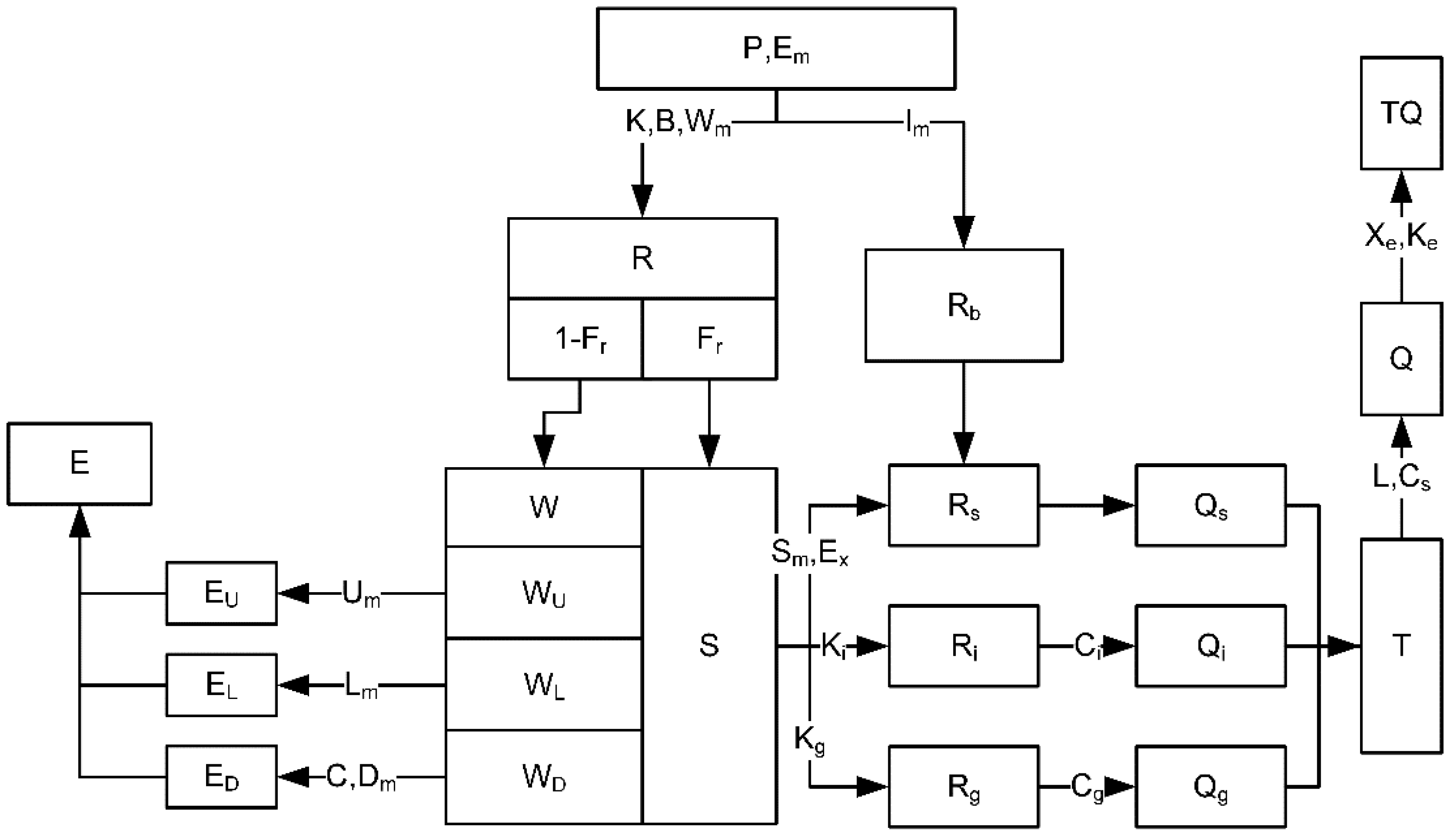
The model used in this study is the Xinanjiang (XAJ) rainfall-runoff model, which is a physically based conceptual hydrological model developed by Zhao [20]. The XAJ model consists of a runoff-generating component and a runoff-routing component. The basin is divided into a set of sub-areas, and runoff is first transformed into discharge by a linear system calculated from the water balance component. The outflow hydrograph from each sub-area is finally routed down the channels to the basin outlet by the Muskingum method. Figure 2 illustrates the model structure, including nine runoff-generating component parameters: the capacity of upper, lower, and deepest soil layers Um, Lm, and Dm, respectively; the impervious area of the sub-basin Im; the areal mean free water storage capacity Sm; the ratio of potential evapotranspiration to pan evaporation K; the exponent of the tension water capacity curve B; the coefficient of deep evapotranspiration C; the runoff-producing area Fr; as well as ten runoff routing component parameters: outflow coefficients of the free water storage to groundwater and interflow Kg and Ki, respectively; recession constants of groundwater, interflow, and channel system Cg, Ci, and Cs, respectively; Muskingum parameters Ke and Xe; the lag time of routing L. For a detailed explanation of the parameters, readers should refer to [20].

2.3. Kernel-Based Residual Error (KRE) Model

We consider a deterministic hydrological model:
y ^ t = f ( X t ; θ h )
that provides the flow forecast y ^ t as a function of the observed forcing data in the vector X t and a model parameter vector θ h . As errors in multiple sources affect the forecast simultaneously [21], the actual flow will be given by
y t = y ^ t + e t
where e t is the raw residual at time t. In hydrologic applications, the raw residuals often exhibit temporal correlation, nonconstant variance (heteroscedasticity), and nonnormality [5,22]. To fully capture the statistical characteristics of the residuals with minimum assumptions, a nonparametric additive structure is adopted:
e t = m n ( R t ) + σ n ( R t ) δ t
where m n ( x ) = E ( e t | R t = x ) is the nonparametric kernel regression function, σ n ( x ) is the conditional volatility (CV) satisfying that σ n 2 ( x ) = Var ( e t | R t = x ) , R t represents the value of the regressor at time t, and δ n is a random variable that follows an unknown distribution with E ( δ t | R t ) = 0 and Var ( δ t | R t ) = 1 .
We adapt a residual-based estimator [23] to estimate m n ( · ) and σ n 2 ( · ) successively. First, the kernel regression function m n ( · ) is estimated using the Adaptive Nadaraya–Watson (ANW) estimator [24],
m ^ n ( x ) = t = 1 n K ( x R t h m ( R t ) ) e t n h m ( R t ) 1 n t = 1 n K ( x R t h m ( R t ) ) 1 h m ( R t )
where x is the given regressor value and n is the sample length of the residual in the calibration period. The kernel smoothing function K adopted in this study is the Gaussian kernel. For standard kernel density estimation problems, constant optimal bandwidths tend to be inadequate when estimating heavily skewed distributions [25] that are frequently observed in hydrological data series due to nonnegativity. To accommodate the statistical characteristics of hydrological data, we use the Abramson-type adaptive bandwidth selector [26] instead of constant optimal bandwidth. The adaptive bandwidth selector provides variable bandwidth h m ( R t ) for different regressor values when estimating the regression function as
h m ( R t ) = h N { f ˜ ( R t ) / g } α m
where f ˜ ( R t ) = 1 n h t = 1 n K ( x R t h ) is the prior kernel estimator with a fixed bandwidth h = 1.06 s n 0.2 , s is the standard deviation of the considering regressor [27], and g (assuming g ≠ 0) is the geometric mean of f ˜ ( R t ) . The exponential parameter αm is called the sensitivity parameter, which satisfies 0 ≤ αm ≤ 1. The adaptive bandwidth selector reduces to the fixed bandwidth when αm = 0 and equals to the nearest neighbor estimator when αm = 1.
The conditional variance function can then be estimated with
σ ^ n 2 ( x ) = t = 1 n K ( x R t h σ ( R t ) ) d t n h σ ( R t ) 1 n t = 1 n K ( x R t h σ ( R t ) ) 1 h σ ( R t )
where d t = ( e t m ^ n ( R t ) ) 2 and h σ ( R t ) is the variable bandwidth for σ ^ n 2 ( · ) given the sensitive parameter ασ according to Equation (6).
Following Evin et al. [28], the AR (1) model is applied to the standardized residual δ n , t to capture the temporal dependency:
δ t = φ δ t 1 + ε t
The temporally independent innovation ε in Equation (7) is approximated by a location-mixture Gaussian distribution, whose density is given by
f ( x ; b ) = 1 n j = 1 n 1 b ϕ ( x ε t b )
where ϕ ( · ) is the probability density function of the standard Gaussian distribution, and b is the estimate of the constant innovation bandwidth. The parameters of the KRE model can then be collectively denoted as θ k = { α m , α σ , b , φ } .

2.4. Residual-Oriented Antecedent Precipitation Index (RAPI)

The RAPI adopts the same expression as the antecedent precipitation index presented by Kohler and Linsley [18] to summarize the antecedent moisture condition:
R A P I = t = 1 M P t k t
where Pt is the precipitation in the tth antecedent hour, M is the statistical number of antecedent hours involving the estimation of RAPI, and k is the decay constant. The parameters of the RAPI model are then θ A = { k , M } .
The value of the RAPI depends on both M and k. Larger values of the two parameters produce a larger value of the RAPI. To find the optimal parameter set that links the antecedent moisture condition to the flood residual, we estimate θ A and θ k simultaneously. Details of the calibration method are presented in Section 2.6.

2.5. Calibration Method

2.5.1. The MI-LXPM Algorithm

The estimation of θ h and θ A is complicated because of the integer restriction of the lag parameter L and antecedent hour number M. The MI-LXPM algorithm is a real coded genetic algorithm proposed for solving integer and mixed-integer constrained optimization problems [29]. The algorithm modifies and extends the Laplace crossover and power mutation for integer decision variables. Moreover, a special truncation procedure for the satisfaction of integer restriction on decision variables and a ‘parameter-free’ penalty approach are used in the MI-LXPM algorithm for handling constraints.

2.5.2. Two-Stage Calibration Procedure

A two-stage calibration is applied in this study. The XAJ model is first calibrated by maximizing the Nash–Sutcliffe Efficiency (NSE) [30] using the MI-LXPM algorithm. The NSE is expressed as
NSE ( y ^ , Q ˜ ) = 1 t = 1 n ( y ^ t Q ˜ t ) 2 t = 1 n ( Q ˜ t Q ¯ ) 2
where Q ¯ is the mean of flow observations Q ˜ . The raw residual e t can then be derived by Equation (2).
The parameters of the KRE and RAPI model { θ A , θ k } are estimated in the second stage. The standardized residual δ t can be calculated by substituting the RAPI estimates into Equations (4) and (5). As the temporal autocorrelation structure of δ t is assumed to be captured by the AR(1) model, the ‘leave-one-out’ kernel likelihood function [31] of the raw residual e can be expressed as
L k ( e | θ A , θ k ) = t = 1 n [ 1 σ n , t ( n 1 ) j = 1 j t n 1 b ϕ ( ε j ε t b ) ]
where σ n , t is the conditional volatility (CV) at time t given the estimated RAPI value according to Equation (6). The MI-LXPM algorithm in Section 2.5.1 can then be implemented to find the optimal values of { θ A , θ k } that minimize the negative log-likelihood function derived from Equation (11).

2.6. Probabilistic Predictions

The probabilistic streamflow predictions are critical when analyzing the flood prediction uncertainty structure and evaluating the rationality of the stochastic framework. The predictive distribution of streamflow y ˘ is given by combining the deterministic model output y ^ t and the residual replicates generated from the KRE model. At a given time step t, the generating process can be described as follows:
(1)
Sample innovations from the inverse of the estimated innovation distribution in Equation (8):
ε t ( r ) F 1 ( ε | b )
(2)
Model temporal structure with Equation (7):
δ t ( r ) = φ ^ δ t 1 ( r ) + ε t ( r )
Note that we set the raw residual replicates at the first time step as δ 1 ( r ) = ε 1 ( r ) .
(3)
Calculate the value of regression function m ^ n ( · ) and CV function σ ^ n ( · ) by substituting the corresponding regressor R t into Equations (4) and (6) sequentially.
(4)
Generate samples of e t ( r ) using Equation (3):
e t ( r ) = m ^ n ( R t ) + σ ^ n ( R t ) δ t ( r )
(5)
Combine with the deterministic model output y ^ t
y t ( r ) = y ^ t + e t ( r )
Then, all predictive replicates constitute the distribution of the predicted flow:
y = { y t ( r ) ; t = 1 , , n ; r = 1 , , N r }
where N r stands for the number of replicates. We set N r = 10 , 000 for all flood event predictions made in this paper

2.7. Probabilistic Prediction Performance Metrics

The reliability and precision metric [6] are used in this work to evaluate the performance of the marginal probabilistic predictions in the time domain. The Nash–Sutcliffe Efficiency is used to measure the bias of point estimates for both hydrological model output and stochastic simulations. The error-correction ability of the error models can then be compared through these two results. In addition to these performance metrics, we use the predictive quantile-quantile (PQQ) plot [32] to assess the reliability of the prediction distribution of streamflow visually.

2.7.1. Reliability Metric

The reliability metric quantifies the statistical consistency of a predictive distribution and the observation. It is numerically calculated as
π [ Y , Q ˜ ] = 2 n t = 1 n | F U [ F Y ( t ) ( Q ˜ t ) ] F Ω [ F Y ( t ) ( Q ˜ t ) ] |
where F Y ( t ) is the cdf of the predictive distribution at time t, F U is the cdf of the uniform distribution U(0, 1), and F Ω is the empirical cdf of Ω = { F Y ( t ) ( Q ˜ t ) , t = 1 , , n } .
A reliability metric value of 0 represents that the PQQ plot follows the 1:1 line, thus the perfect reliability. On the opposite, the value 1 represents the worst reliability. The metric in Equation (17) is used frequently in the hydrological modeling literature to assess the reliability of time-varying prediction distributions [4,8,33].

2.7.2. Precision Metric

Precision refers to the width or spread of the probabilistic prediction. A precision metric is quantified using
P c [ Y , Q ˜ ] = 1 n t = 1 n std ( Y t ) 1 n t = 1 n Q ˜ t
where std ( Y t ) is the standard deviation of the predictive replicates at time t, { y t ( r ) ; t = 1 , , n } . Equation (18) measures the ‘average’ standard deviation across all evaluated periods, scaled by the observation mean to compare different catchments. A lower value of the precision metric ensures good prediction sharpness. The precision metric does not depend on how well the probabilistic predictions reproduce the actual observation. Thus, the reliability and precision metric should be considered together to evaluate probabilistic predictions.

3. Results and Discussion

Following the stochastic framework and calibration strategy presented in Section 2, this study investigates the influence of the soil moisture condition on the uncertainty of flood prediction. The soil moisture condition is approximated by the RAPI, whose parameters are calibrated with the KRE model simultaneously.
The residual sample e is derived after the first-stage calibration of the XAJ model. Prior limits and optimal estimates of the XAJ model parameters are shown in Table 1. Only 11 XAJ model parameters are chosen to be calibrated by the ‘Maximum-NSE’ criteria, while others are pre-determined empirically following [20]. Based on the geo-morphological lumping nature of the XAJ model, the rainfall-runoff process of the Changshangang River Basin is aggregated into one single cell with equivalent hydrological properties. On the other hand, consistent with the hydrometeorological observations, the time step of the flood simulation is one hour.
In the second-stage calibration, the KRE and RAPI model parameters are estimated by minimizing the negative log-likelihood function value according to Equation (11). Meanwhile, to further evaluate the predictive performance of RAPI on flood prediction uncertainty, the deterministic model output y ^ is chosen as another regressor of the KRE model, which is common practice in the hydrological modeling literature [9,34,35]. We call the two scenarios ‘KA’ and ‘KF’ corresponding to the regressors RAPI and y ^ . As y ^ is fixed after the first-stage calibration, the ‘KF’ scenario only has three parameters of the KRE model. The prior setting and optimal parameters of the two modeling scenarios are listed in Table 2.

3.1. Flood Prediciton Residuals and RAPI Estimates

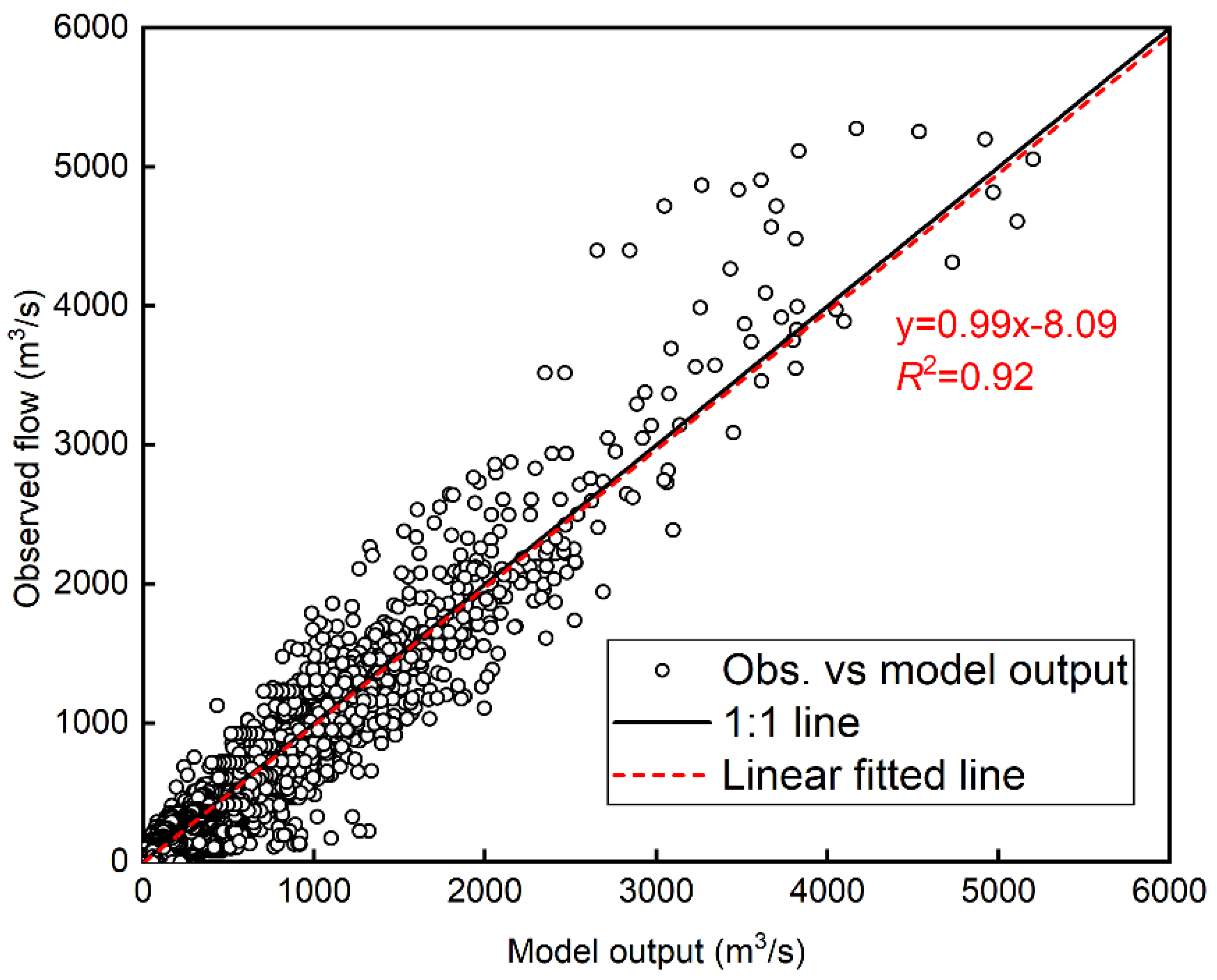
Given the optimal parameters in Table 1, the XAJ model reproduces the hourly streamflow relatively well for all flood events in the Changshangang River Basin, with a mean NSE value of 0.82. Figure 3 shows the one-to-one correspondence between the simulated streamflow and the observations. The fitted linear trend of the scatter plot is close to the 1:1 line for the most part with an R-squared value of 0.92. However, clusters in the upper right corner above the 1:1 line mean that the XAJ model underestimates the extreme flood peaks. On the contrary, opposite trends in the lower left corner indicate that the XAJ model overestimates low flow periods of the selected flood events. Moreover, the ‘fanning-out’ pattern of the scatter plot suggests heteroscedasticity of the residuals for different streamflow magnitudes.
According to Table 2, the optimal RAPI is the weighted average precipitation of the preceding 51 h. Compared to the XAJ lag parameter L (6 h, according to Table 1), the RAPI shows a longer time scale than the forcing precipitation. A decay constant of 0.97 implies that the impact of precipitation decreases slowly with the antecedent time, providing a minimal weight of 0.21 for the earliest time step.
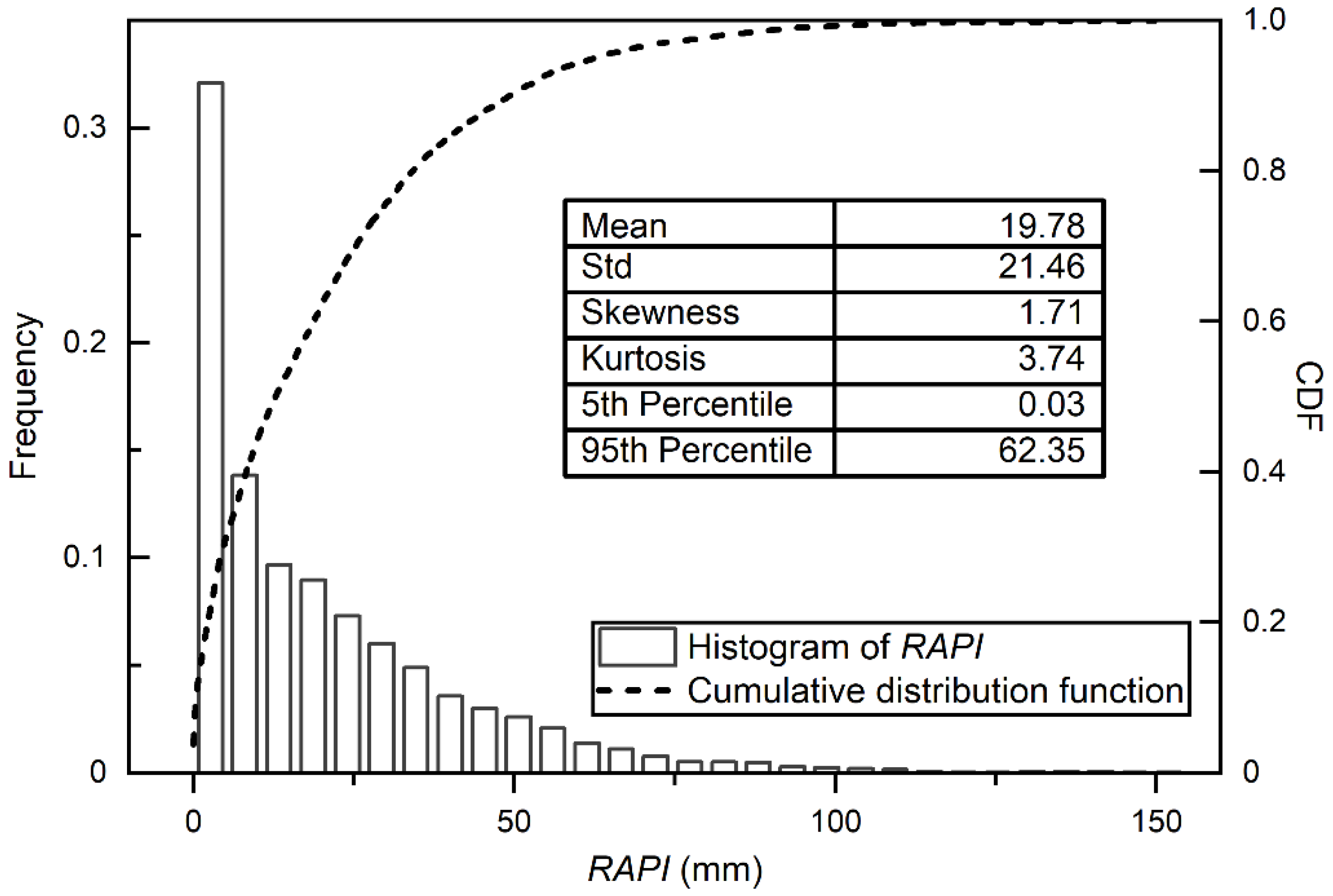
Figure 4 summarizes the statistical characteristics of the optimal RAPI. The optimal RAPI ranges between 0 mm and 149.82 mm, with a mean of 19.78 mm. The nonnegative nature of the precipitation leads to the positive skewness of RAPI. Moreover, a kurtosis of 3.74 (0 for Gaussian distribution) implies outliers in the right tail, consistent with the significant deviation between the mean and 95th percentile of RAPI.
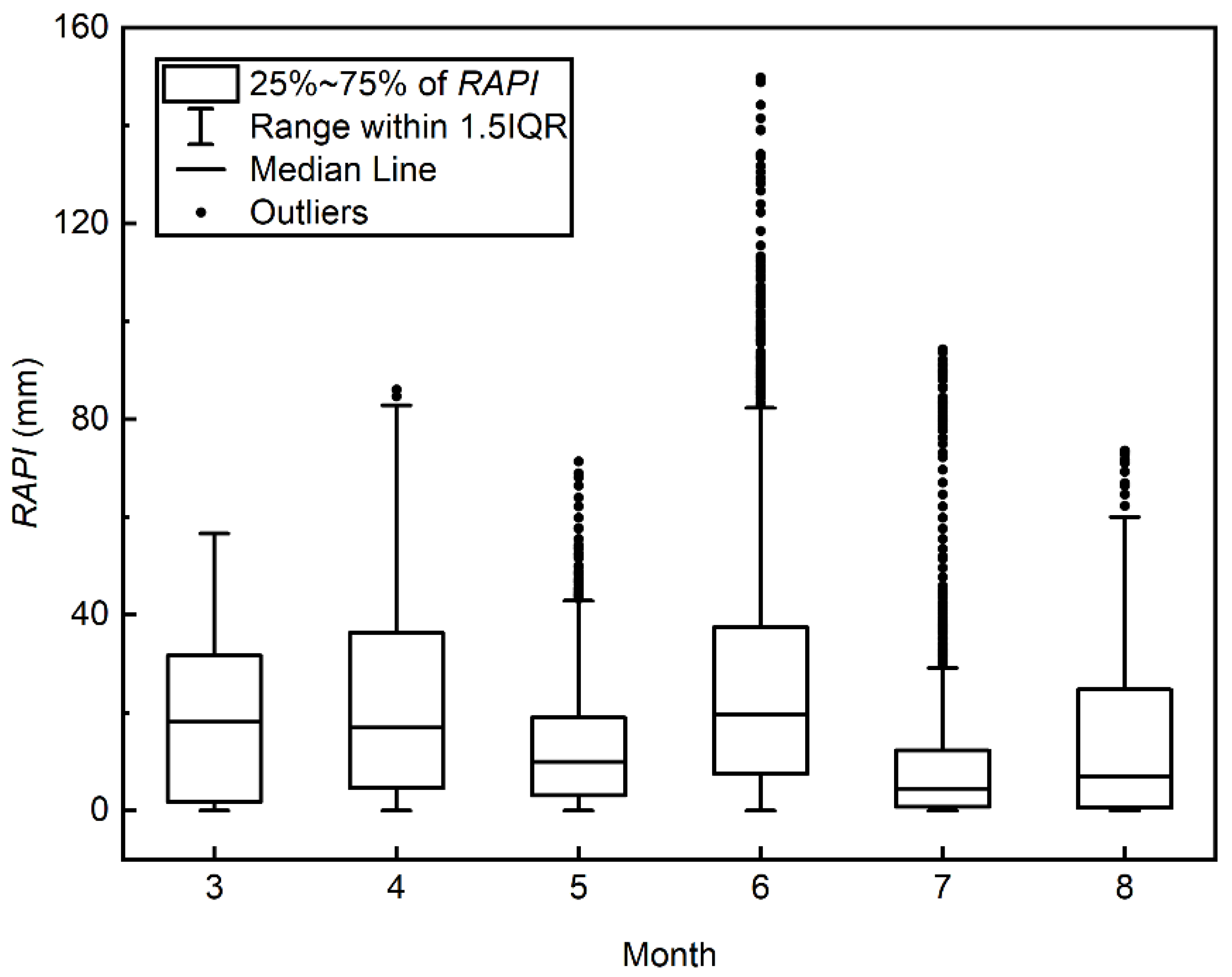
Distributions of the optimal RAPI in different months are shown in Figure 5. Most outliers of the optimal RAPI occur in June, which possesses the most precipitation of the year. In addition to June, optimal RAPI samples in March and April possess the largest median value, suggesting that larger soil moisture is necessary for flood events to occur in months with less precipitation.
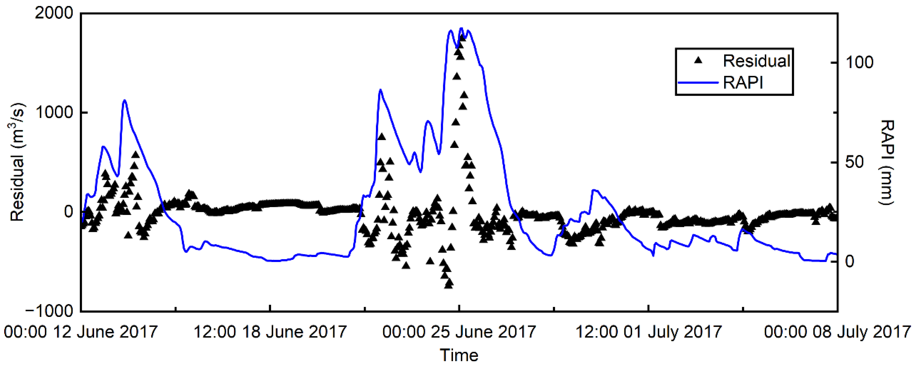
A representative example of the residual and RAPI time series is presented in Figure 6. The chosen flood event from 12 June 2017 to 8 July 2017 contains the largest flood peak volume (4870 m3/s at 23:00 24 June 2017) and absolute residual value (1746 m3/s at 2:00 25 June 2017). Figure 6 shows that lower values of the optimal RAPI correspond to stable residuals near zero, while a larger RAPI follows with strong fluctuations in residuals. This phenomenon suggests that the optimal RAPI can capture the heteroscedasticity of the residual.

3.2. Impact of the Optimal RAPI on Flood Residual

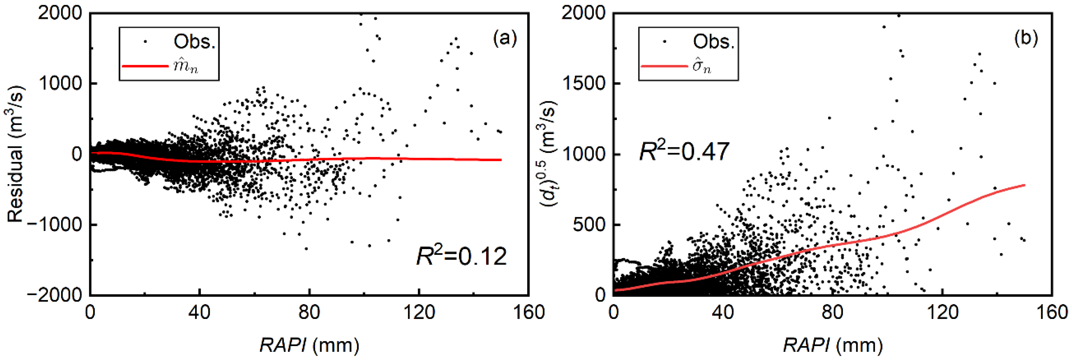
Figure 7a shows the optimal kernel regression of the flood residual given the regressor of RAPI. After a slight ascending trend, a mild descending trend appears in the regression function. When RAPI < 14.09 mm, the regression function of the residual is above zero, implying an underestimation of the XAJ model under low-soil-moisture conditions and vice versa. Moreover, an R-squared value of 0.12 implies that the estimated RAPI cannot fully explain the expectation of raw flood residuals.
On the other hand, the CV function in Figure 7b rises with an increasing gradient over the optimal RAPI value. A minimal CV value of 38.2 m3/s corresponds to the lowest RAPI of 0 mm, while a maximum CV value of 782.5 m3/s corresponds to the largest RAPI of 149.82 mm. The increasing trend in the CV function of the residual suggests that the predictive uncertainty magnifies almost 20 times between the minimal and maximum optimal RAPI value. A relatively high R-squared value of 0.47 suggests that RAPI provides an adequate representation of changes in the CV function of flood residuals.
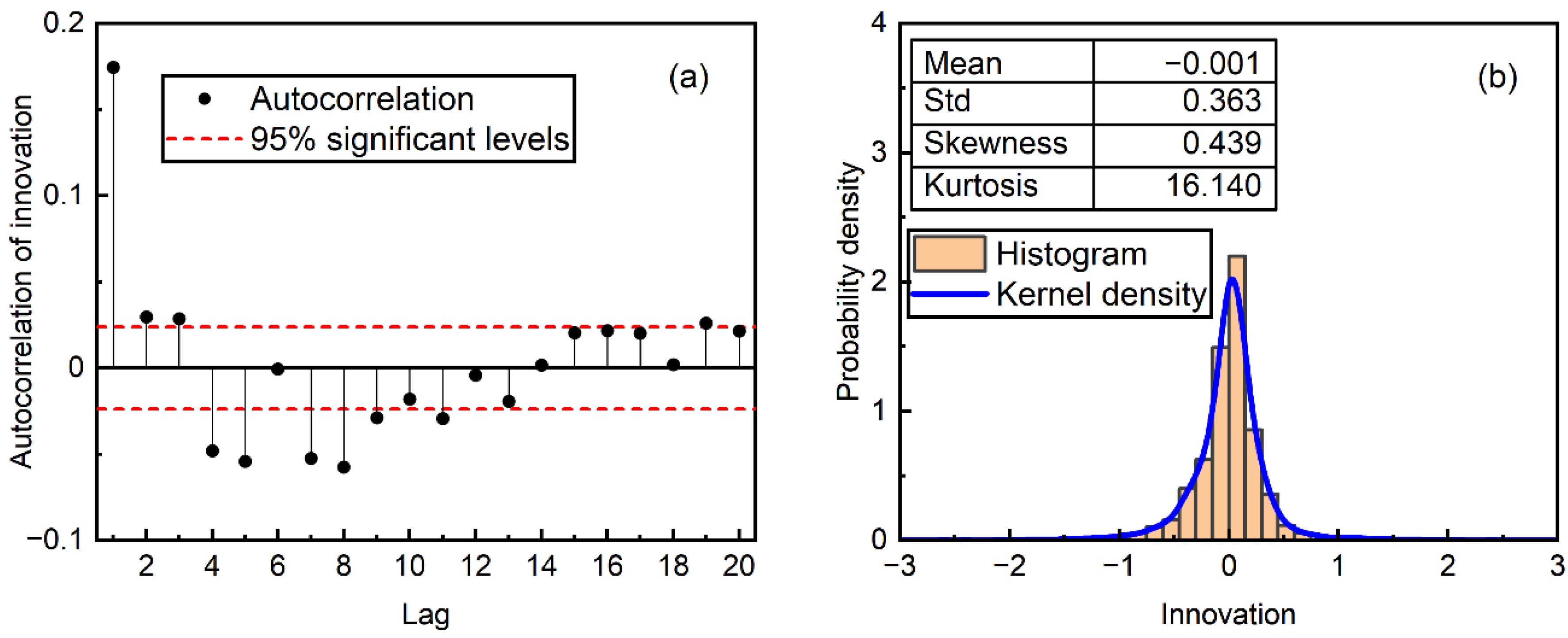
After applying the KRE model, the standardized residual of the ‘KA’ scenario presents a first-order autocorrelation coefficient of 0.93 (Table 2), which can be attributed to the memory effect of XAJ residuals [21] and the imperfection of the KRE model. Nevertheless, the AR (1) model captures the temporal autocorrelation structure relatively well, only leaving permissible dependence in the first lag. Note that the standard deviation of the innovation ε is 0.36, as shown in Figure 8b, which leads to a close-to-one standard deviation of δ n (as std ( ε ) = std ( δ n ) 1 φ 2 ). This result further verifies the assumption of the KRE model.
The distribution of the innovation is distinct from the Gaussian distribution, especially for its excessive kurtosis (Figure 8b). This phenomenon is also reported in [5], demonstrating the necessity of applying a more flexible distribution model such as the location-mixture Gaussian in this study.

3.3. Stochastic Predictive Performance

As shown in Table 3, the two modeling scenarios perform similarly with respect to probabilistic predictions considering their relative metric values. The ‘KA’ scenario outperforms the ‘KF’ scenario in likelihood and precision, suggesting more sharpness in the flood prediction uncertainty bands (PUBs) and more reliable assumptions on the residual. On the other hand, the ‘KF’ scenario gains a higher value of NSE S ¯ , implying better bias-correction ability.
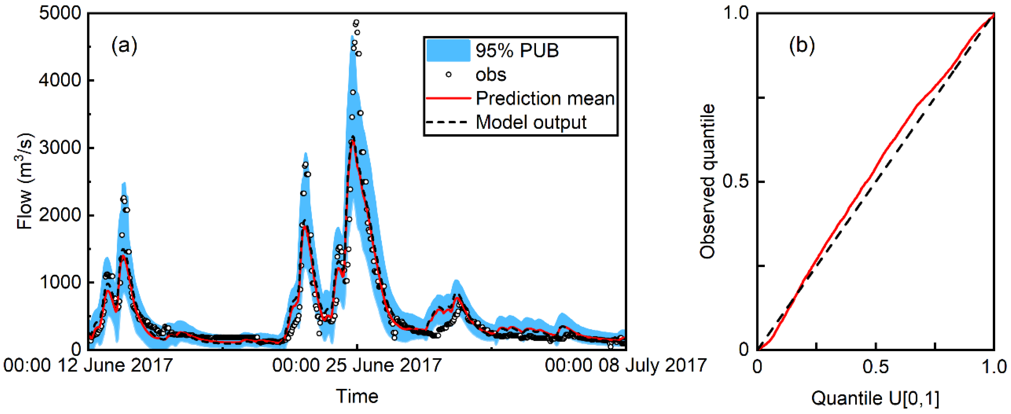
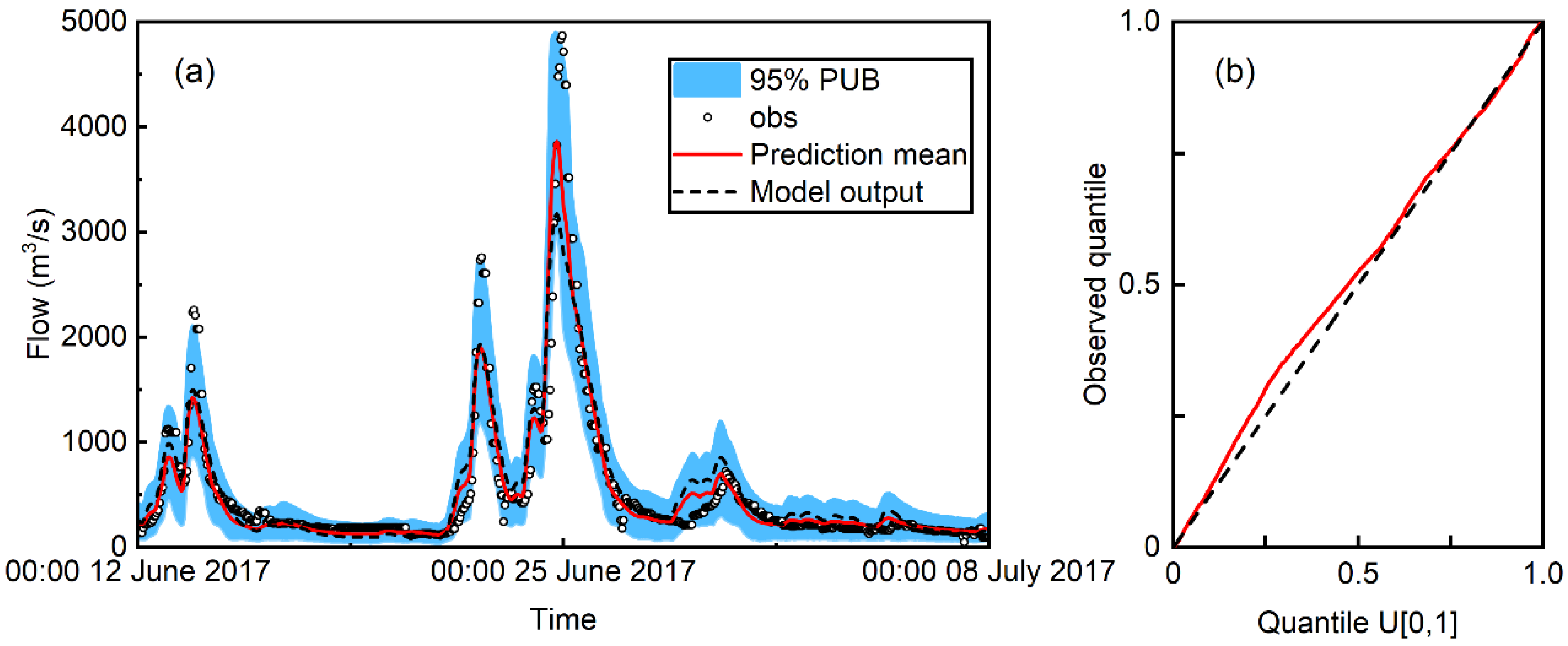
The almost overlapping lines of the prediction mean and deterministic model output in Figure 9 proves the identical value of NSE S ¯ and NSE for the ‘KA’ scenario. The flat regression function in Figure 7a explains t as a poor bias-correction performance, especially for extreme flood peaks with significant underestimation.
The 95% PUB for the ‘KA’ scenario covers the flood observations well, except for the highest flow observations from 23:00 24 June 2017 to 05:00 25 June 2017 (Figure 9a). It is noteworthy that all flow peak observations in the other 21 flood events are within the range of 95% PUB for the ‘KA’ scenario. Furthermore, observations of flood peaks are found clustering near the upper limit of the 95% PUB, showing a trend of under-prediction. The PQQ plot in Figure 9b lies above the 1:1 line, again proving the under-prediction trend of the ‘KA’ scenario.
The similarity of Figure 9 and Figure 10 confirms the findings from the performance metric values in Table 3. One of the differences between the two modeling scenarios is that the ‘KF’ scenario produces a better correction of the flood peak prediction., which explains its higher value of NSE S ¯ . However, the better bias-correction ability of the flood peaks is still insufficient to mitigate the overall underestimation trend of the ‘KF’ scenario according to the PQQ plot (Figure 10b). Moreover, a more expansive PUB of the ‘KF’ scenario suggests the overestimation of uncertainty. This deficit can be attributed to the regressor y ^ t , which cannot distinguish the high prediction uncertainty caused by the forcing precipitation from the low prediction uncertainty of a pure recession period [12].

3.4. Impact of Soil Moisture on Predictive Performance of Flood

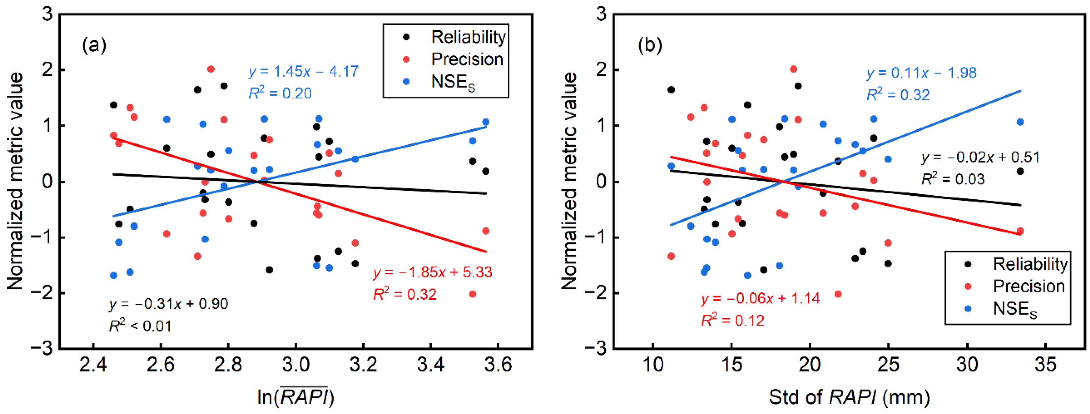
As the RAPI is the proxy of the antecedent soil moisture condition, we investigate the impact of soil moisture on flood prediction performance by comparing the normalized performance metric values under different RAPI conditions. The mean optimal RAPI is chosen to represent the average soil moisture condition during flood events (a natural logarithm is implemented to strengthen the linear trend). At the same time, the standard deviation of RAPI is used to represent the variation in soil moisture. Results are shown in Figure 11.
The evenly distributed markers of reliability metrics in both Figure 11a,b lead to flat linear trends with negligible R-squared values. This finding suggests that antecedent soil moisture has little effect on the reliability of the probabilistic flood predictions.
On the other hand, both the precision metric and NSES illustrate statistically significant linear trends. According to the definition of the two metrics, although given opposite trends, the result suggests improved predictive precision and unbiasedness. In the comparison of Figure 11a,b, the unbiasedness of flood prediction is found to be more sensitive to the variation in soil moisture. At the same time, the predictive precision is more sensitive to the volume of soil moisture.
The relatively poor bias-correction ability of the ‘KA’ scenario (see Section 3.3) suggests the improvement of unbiasedness. This improvement is mainly due to the deterministic model output when facing abundant and fluctuating soil moisture. Unlike unbiasedness, the reason for improved prediction precision can be twofold: (1) The improved unbiasedness provides more stable and smaller residuals, and (2) the KRE model can better reproduce residuals in such soil moisture conditions. The second reason can be proved by investigating the distribution of the optimal RAPI in Figure 4. Though applying the adaptive bandwidth, the over-cluster of the optimal RAPI samples in low-value regions still causes an over-smoothness of kernel regression and the CV function (see Figure 7), reducing the effectiveness of the kernel estimator. As a result, lower RAPI values correspond to worse predictive performances.

3.5. Comparison of the Regressor

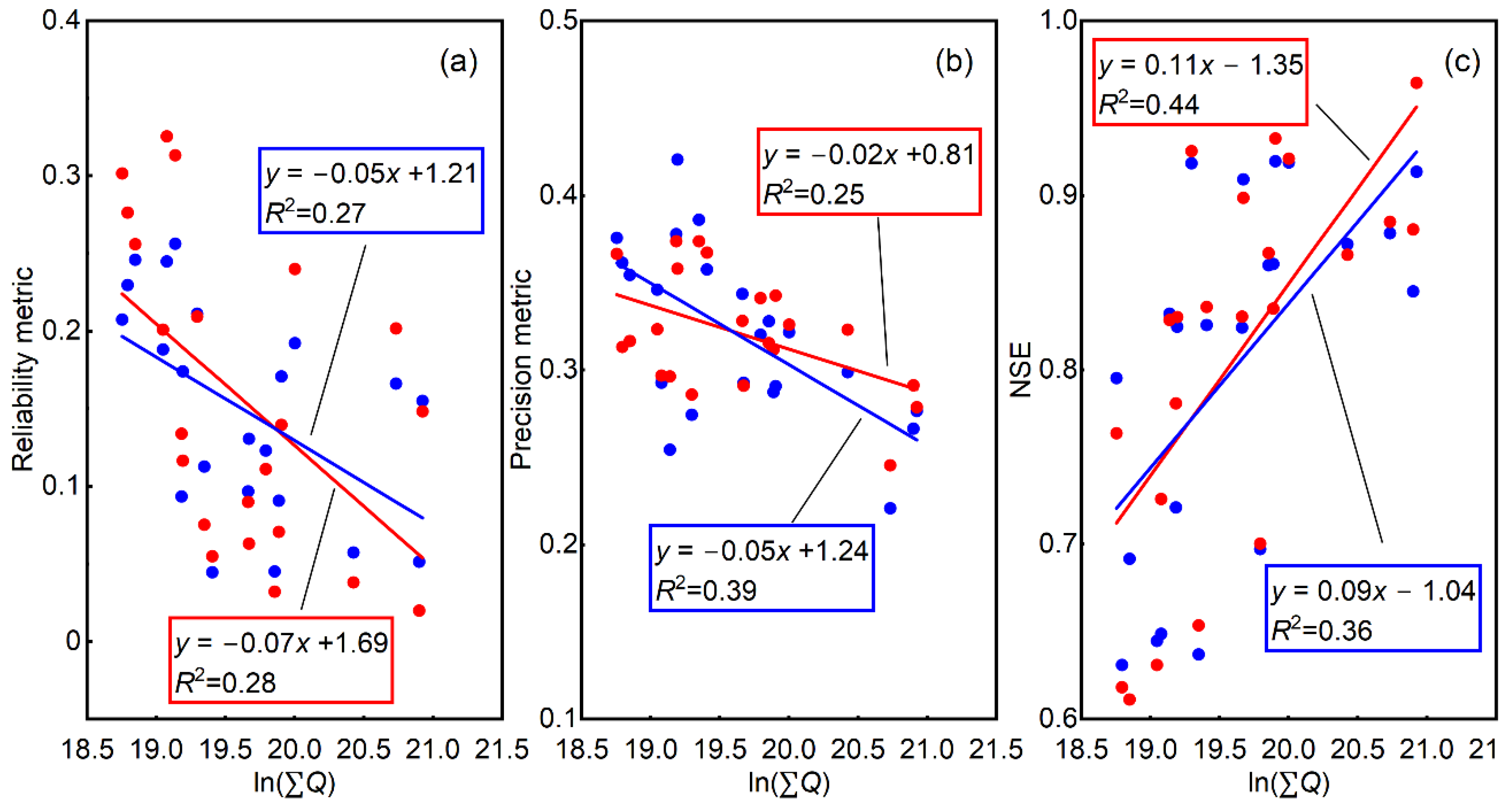
To further evaluate the correspondence of the proposed RAPI toward flood prediction uncertainty, we compare the predictive performance metrics of both modeling scenarios under different flood magnitudes. Statistically significant improving trends are shown in all three metrics for the two modeling scenarios, according to Figure 12.
As larger values of the standard deviation of RAPI often correspond to serious flood events with larger total volumes, the reasons for improved predictive performance with increasing flood volume are similar to those with increasing RAPI for both modeling scenarios. In fact, as a regressor, the deterministic model output y ^ possesses more significant kurtosis (25.03) and skewness (3.93) than the RAPI, leading to more severe clustering in low flow values. As a result, both reliability and unbiasedness of the ‘KF’ scenario under-perform those of the ‘KA’ scenario in lower flood volume conditions.
The cross point of fitted reliability lines appears in ln Q = 19.80 , implying that the ‘KA’ scenario prediction is more reliable in 63% of all flood events with lower flood volume. Similarly, the ‘KA’ scenario outperforms the ‘KF’ scenario in the lower 50% of flood events. With the homologous performance in precision for both scenarios, this finding suggests that the RAPI is more critical than y ^ in estimating predictive uncertainty for less extreme flood events. Bennett et al. reported a similar conclusion in [13].
On the contrary, the ‘KF’ scenario provides better stochastic predictions when dealing with extreme flood events, implying better correspondence between y ^ and residuals of extreme flood events than RAPI. As extreme flood events in the Changshangang River Basin are mainly caused by short-time heavy rainfall, the superiority of y ^ may be due to its inclusion of forcing precipitation.
Considering the performances of the ‘KA’ and ‘KF’ scenarios, practitioners can choose the regressor based on relative flood volume. Further investigation of multi-variate modeling of y ^ and RAPI is recommended based on their complementary predictive performances.

3.6. Limitations and Future Work

The major limitation of this study is the neglect of rainfall uncertainty. The hourly mean areal precipitation calculated from rain gages is assumed to be the ‘true input’ of the XAJ, RAPI, and KRE models. In this way, the computational complexity of the likelihood function (Equation 11) is significantly reduced. However, the rainfall estimates are inherently uncertain due to inadequate areal coverage of gaging sites, inaccurate spatial-temporal interpolation, mechanical limitations of pluviometers, etc. [36]. As the hydrological systems are heavily input-driven [37,38,39], inaccurate rainfall characterization can impair the quality of calibration and prediction results [40,41].
While this study does not consider the influence of rainfall uncertainty, it does substantiate that antecedent accumulated rainfall has a critical impact on flood prediction uncertainty. A natural progression of this work is to make the input rainfall uncertain and to propagate it through the entire flood prediction process. As a simple but robust solution, the so-called rainfall multiplier [42] can generate event-specific random variables that can be multiplied with the rainfall observation to provide random rainfall input. Then, the multipliers and their uncertainty are estimated jointly with all other model parameters to correct possible flood prediction errors and account for the total predictive uncertainty.

4. Conclusions

Antecedent moisture conditions are widely assumed to be essential in explaining differences in the translation of flood-producing precipitation to floods. However, there still lacks a general framework to estimate and further link it with flood predictive uncertainty. Instead of implementing physical-based models, this study proposes an empirical model only based on antecedent precipitation.
Despite the same structure as the API, the proposed RAPI differs in the calibration procedure. This paper adopts a fully kernel-based residual error model without functional presumptions, thus being data-driven. The RAPI is then calibrated simultaneously with the KRE model as the regressor. Furthermore, the MI-LXPM algorithm is applied to search for optimal parameters in mixed-integer constraints.
The rationality of the proposed framework is demonstrated by its application to a case study in South-East China. The quality of probabilistic streamflow predictions is then quantified using reliability, precision, and the NSE of the prediction mean. The key findings of the paper are as follows:
  • For hourly flood predictions, the optimal RAPI can be the weighted average of hourly precipitation falls in the antecedent days with a mild decay. The distribution of the optimal RAPI is found to be highly peaked with positive skewness.
  • The optimal RAPI influences the residual conditional volatility more than the conditional mean. As a result, a poor bias-correction ability can be found when making probabilistic flood predictions with RAPI.
  • The reliability of probabilistic flood prediction is almost independent of the RAPI value. On the contrary, prediction precision and unbiasedness are found to improve with increasing value and variability of the RAPI.
  • As a regressor, the RAPI produces better probabilistic flood predictions for small to median flood events than the deterministic model output y ^ . On the contrary, y ^ provides better predictions of extreme flood events.
As a proxy of antecedent soil moisture, the RAPI closely connects to the uncertainty of hourly flood prediction. Along with the proposed data-driven residual error model, the framework can be applied to any pre-calibrated hydrological model and help modelers achieve high-quality probability flood prediction. Further research is recommended to determine the influence of rainfall uncertainty on both the RAPI and flood predictive uncertainty.

Author Contributions

Conceptualization, J.L.; methodology, J.L. and Z.H.; software, J.L.; validation, J.L., S.L. and Z.H.; formal analysis, J.L.; investigation, J.L., Y.Z. and G.Z.; resources, S.L.; data curation, J.L.; writing—original draft preparation, J.L.; writing—review and editing, A.N.M. and J.T.A.; visualization, J.L.; supervision, S.L.; project administration, S.L.; funding acquisition, S.L. All authors have read and agreed to the published version of the manuscript.

Funding

This study was financially supported by the National Key R&D Program of China (Grant no. 2018YFD1100401) and the National Natural Science Foundation of China (51961145106).

Data Availability Statement

Hydrological data used in this paper can be found at https://www.researchgate.net/publication/363144895_data_for_changshangang (accessed on 30 August 2022).

Acknowledgments

We are grateful to the editors and four anonymous reviewers for their thoughtful comments on this manuscript.

Conflicts of Interest

The authors declare no conflict of interest.

References

  1. Beven, K.; Binley, A. The future of distributed models: Model calibration and uncertainty prediction. Hydrol. Process. 1992, 6, 279–298. [Google Scholar] [CrossRef]
  2. Del Giudice, D.; Honti, M.; Scheidegger, A.; Albert, C.; Reichert, P.; Rieckermann, J. Improving uncertainty estimation in urban hydrological modeling by statistically describing bias. Hydrol. Earth Syst. Sci. 2013, 17, 4209–4225. [Google Scholar] [CrossRef] [Green Version]
  3. Reichert, P.; Ammann, L.; Fenicia, F. Potential and Challenges of Investigating Intrinsic Uncertainty of Hydrological Models with Stochastic, Time-Dependent Parameters. Water Resour. Res. 2021, 57, e2020W–e28400W. [Google Scholar] [CrossRef]
  4. Renard, B.; Kavetski, D.; Kuczera, G.; Thyer, M.; Franks, S.W. Understanding predictive uncertainty in hydrologic modeling: The challenge of identifying input and structural errors. Water Resour. Res. 2010, 46, 1–22. [Google Scholar] [CrossRef]
  5. Schoups, G.; Vrugt, J.A. A formal likelihood function for parameter and predictive inference of hydrologic models with correlated, heteroscedastic, and non-Gaussian errors. Water Resour. Res. 2010, 46, w10531. [Google Scholar] [CrossRef] [Green Version]
  6. McInerney, D.; Thyer, M.; Kavetski, D.; Lerat, J.; Kuczera, G. Improving probabilistic prediction of daily streamflow by identifying P areto optimal approaches for modeling heteroscedastic residual errors. Water Resour. Res. 2017, 53, 2199–2239. [Google Scholar] [CrossRef]
  7. Sun, R.; Yuan, H.; Liu, X. Effect of heteroscedasticity treatment in residual error models on model calibration and prediction uncertainty estimation. J. Hydrol. 2017, 554, 680–692. [Google Scholar] [CrossRef]
  8. Evin, G.; Thyer, M.; Kavetski, D.; McInerney, D.; Kuczera, G. Comparison of joint versus postprocessor approaches for hydrological uncertainty estimation accounting for error autocorrelation and heteroscedasticity. Water Resour. Res. 2014, 50, 2350–2375. [Google Scholar] [CrossRef]
  9. Hunter, J.; Thyer, M.; McInerney, D.; Kavetski, D. Achieving high-quality probabilistic predictions from hydrological models calibrated with a wide range of objective functions. J. Hydrol. 2021, 603, 126578. [Google Scholar] [CrossRef]
  10. Li, M.; Wang, Q.J.; Bennett, J.C.; Robertson, D.E. Error reduction and representation in stages (ERRIS) in hydrological modelling for ensemble streamflow forecasting. Hydrol. Earth Syst. Sci. 2016, 20, 3561–3579. [Google Scholar] [CrossRef]
  11. Jiang, X.; Gupta, H.V.; Liang, Z.; Li, B. Toward Improved Probabilistic Predictions for Flood Forecasts Generated Using Deterministic Models. Water Resour. Res. 2019, 55, 9519–9543. [Google Scholar] [CrossRef]
  12. Pianosi, F.; Raso, L. Dynamic modeling of predictive uncertainty by regression on absolute errors. Water Resour. Res. 2012, 48, W03516. [Google Scholar] [CrossRef]
  13. Bennett, B.; Leonard, M.; Deng, Y.; Westra, S. An empirical investigation into the effect of antecedent precipitation on flood volume. J. Hydrol. 2018, 567, 435–445. [Google Scholar] [CrossRef]
  14. Song, S.; Wang, W. Impacts of Antecedent Soil Moisture on the Rainfall-Runoff Transformation Process Based on High-Resolution Observations in Soil Tank Experiments. Water 2019, 11, 296. [Google Scholar] [CrossRef] [Green Version]
  15. Chen, X.; Parajka, J.; Széles, B.; Valent, P.; Viglione, A.; Blöschl, G. Impact of Climate and Geology on Event Runoff Characteristics at the Regional Scale. Water 2020, 12, 3457. [Google Scholar] [CrossRef]
  16. Khatun, A.; Ganguli, P.; Bisht, D.S.; Chatterjee, C.; Sahoo, B. Understanding the impacts of predecessor rain events on flood hazard in a changing climate. Hydrol. Process. 2022, 36, e14500. [Google Scholar] [CrossRef]
  17. Zscheischler, J.; Westra, S.; van den Hurk, B.J.J.M.; Seneviratne, S.I.; Ward, P.J.; Pitman, A.; AghaKouchak, A.; Bresch, D.N.; Leonard, M.; Wahl, T.; et al. Future climate risk from compound events. Nat. Clim. Chang. 2018, 8, 469–477. [Google Scholar] [CrossRef]
  18. Kohler, M.A.; Linsley, R.K. Predicting the Runoff from Storm Rainfall; US Department of Commerce, Weather Bureau: Washington, DC, USA, 1951.
  19. Heggen, R.J. Normalized Antecedent Precipitation Index. J. Hydrol. Eng. 2001, 6, 377–381. [Google Scholar] [CrossRef]
  20. Ren-Jun, Z. The Xinanjiang model applied in China. J. Hydrol. 1992, 135, 371–381. [Google Scholar] [CrossRef]
  21. Kuczera, G.; Kavetski, D.; Franks, S.; Thyer, M. Towards a Bayesian total error analysis of conceptual rainfall-runoff models: Characterising model error using storm-dependent parameters. J. Hydrol. 2006, 331, 161–177. [Google Scholar] [CrossRef]
  22. Yang, J.; Reichert, P.; Abbaspour, K.C.; Yang, H. Hydrological modelling of the Chaohe Basin in China: Statistical model formulation and Bayesian inference. J. Hydrol. 2007, 340, 167–182. [Google Scholar] [CrossRef]
  23. Fan, J.; Yao, Q. Efficient Estimation of Conditional Variance Functions in Stochastic Regression. Biometrika 1998, 85, 645–660. [Google Scholar] [CrossRef] [Green Version]
  24. Ahmed, H.I.E.S.; Salha, R.B.; El-Sayed, H.O. Adaptive weighted Nadaraya–Watson estimation of the conditional quantiles by varying bandwidth. Commun. Stat. Simul. Comput. 2020, 49, 1105–1117. [Google Scholar] [CrossRef]
  25. Wand, M.P.; Marron, J.S.; Ruppert, D. Transformations in Density Estimation. J. Am. Stat. Assoc. 1991, 86, 343–353. [Google Scholar] [CrossRef]
  26. Abramson, I.S. On Bandwidth Variation in Kernel Estimates-A Square Root Law. Ann. Stat. 1982, 10, 1217–1223. [Google Scholar] [CrossRef]
  27. Silverman, B.W. Density Estimation for Statistics and Data Analysis; Chapman & Hall: London, UK, 1986. [Google Scholar]
  28. Evin, G.; Kavetski, D.; Thyer, M.; Kuczera, G. Pitfalls and improvements in the joint inference of heteroscedasticity and autocorrelation in hydrological model calibration. Water Resour. Res. 2013, 49, 4518–4524. [Google Scholar] [CrossRef] [Green Version]
  29. Deep, K.; Singh, K.P.; Kansal, M.; Mohan, C. A real coded genetic algorithm for solving integer and mixed integer optimization problems. Appl. Math. Comput. 2009, 212, 505–518. [Google Scholar] [CrossRef]
  30. Nash, J.E.; Sutcliffe, J.V. River flow forecasting through conceptual models part I—A discussion of principles. J. Hydrol. 1970, 10, 282–290. [Google Scholar] [CrossRef]
  31. Shang, H.L. Estimation of a functional single index model with dependent errors and unknown error density. Commun. Stat. Simul. Comput. 2020, 49, 3111–3133. [Google Scholar] [CrossRef]
  32. Thyer, M.; Renard, B.; Kavetski, D.; Kuczera, G.; Franks, S.; Srikanthan, S. Critical evaluation of parameter consistency and predictive uncertainty in hydrological modeling: A case study using Bayesian total error analysis. Water Resour. Res. 2009, 45, W00B14. [Google Scholar] [CrossRef]
  33. Ammann, L.; Fenicia, F.; Reichert, P. A likelihood framework for deterministic hydrological models and the importance of non-stationary autocorrelation. Hydrol. Earth Syst. Sci. 2019, 23, 2147–2172. [Google Scholar] [CrossRef] [Green Version]
  34. McInerney, D.; Thyer, M.; Kavetski, D.; Bennett, B.; Lerat, J.; Gibbs, M.; Kuczera, G. A simplified approach to produce probabilistic hydrological model predictions. Environ. Model. Softw. 2018, 109, 306–314. [Google Scholar] [CrossRef]
  35. Romero-Cuellar, J.; Gastulo-Tapia, C.J.; Hernández-López, M.R.; Prieto Sierra, C.; Francés, F. Towards an Extension of the Model Conditional Processor: Predictive Uncertainty Quantification of Monthly Streamflow via Gaussian Mixture Models and Clusters. Water 2022, 14, 1261. [Google Scholar] [CrossRef]
  36. Del Giudice, D.; Albert, C.; Rieckermann, J.; Reichert, P. Describing the catchment-averaged precipitation as a stochastic process improves parameter and input estimation. Water Resour. Res. 2016, 52, 3162–3186. [Google Scholar] [CrossRef] [Green Version]
  37. Nanding, N.; Wu, H.; Tao, J.; Maggioni, V.; Beck, H.E.; Zhou, N.; Huang, M.; Huang, Z. Assessment of Precipitation Error Propagation in Discharge Simulations over the Contiguous United States. J. Hydrometeorol. 2021, 22, 1987–2008. [Google Scholar] [CrossRef]
  38. Gao, Y.; Sarker, S.; Sarker, T.; Leta, O.T. Analyzing the critical locations in response of constructed and planned dams on the Mekong River Basin for environmental integrity. Environ. Res. Commun. 2022, 4, 101001. [Google Scholar] [CrossRef]
  39. Sarker, S.; Veremyev, A.; Boginski, V.; Singh, A. Critical Nodes in River Networks. Sci. Rep. 2019, 9, 11178. [Google Scholar] [CrossRef] [Green Version]
  40. Wu, X.; Marshall, L.; Sharma, A. Quantifying input error in hydrologic modeling using the Bayesian error analysis with reordering (BEAR) approach. J. Hydrol. 2021, 598, 126202. [Google Scholar] [CrossRef]
  41. Shimizu, K.; Yamada, T.; Yamada, T.J. Uncertainty Evaluation in Hydrological Frequency Analysis Based on Confidence Interval and Prediction Interval. Water 2020, 12, 2554. [Google Scholar] [CrossRef]
  42. Kavetski, D.; Kuczera, G.; Franks, S. Bayesian analysis of input uncertainty in hydrological modeling: 1. Theory. Water Resour. Res. 2006, 42, W03407. [Google Scholar] [CrossRef]
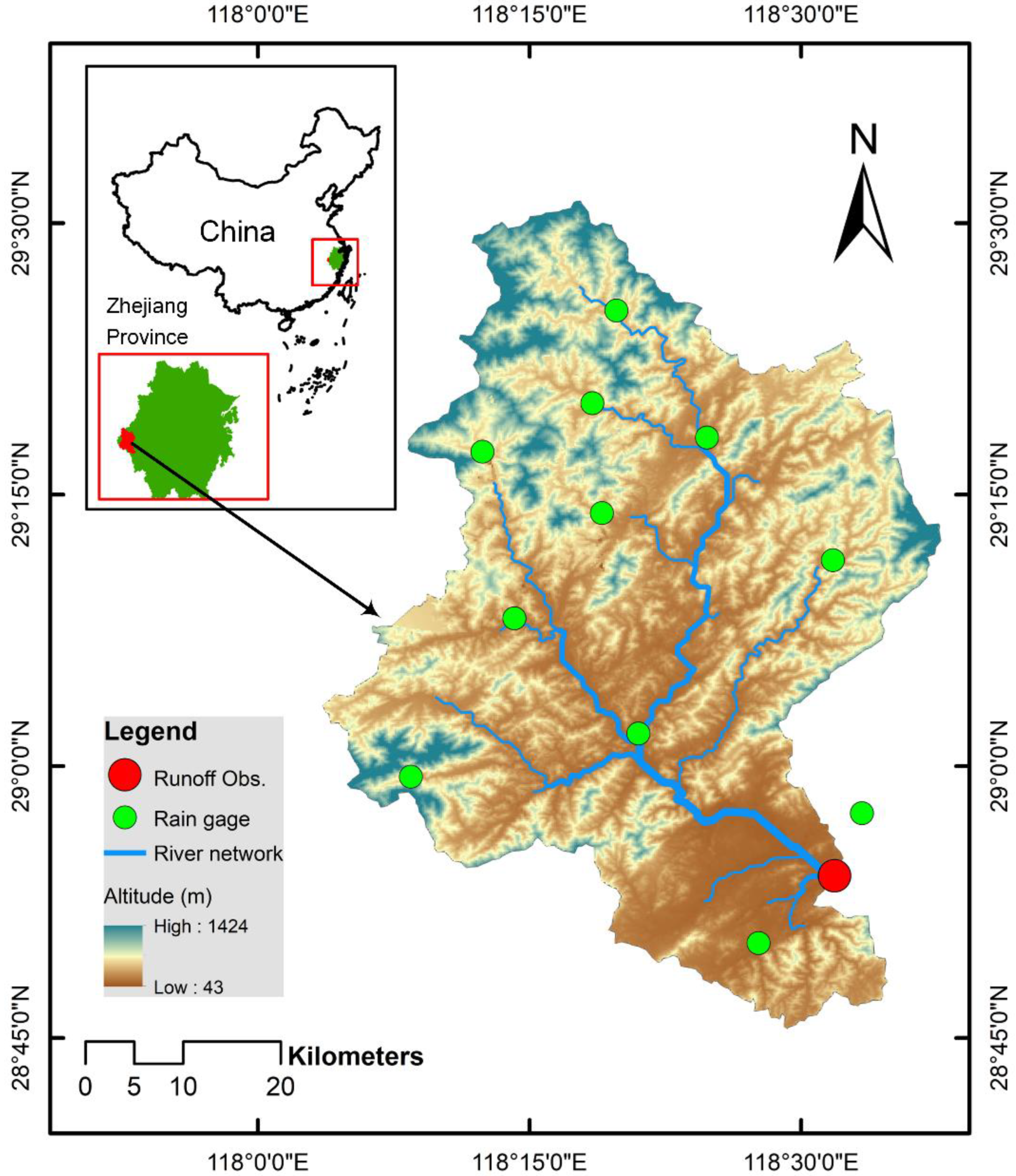
Figure 1. Map of the Changshangang River Basin. Rain gages are shown with green circles, and runoff observations are collected from the Changshangang station (red circle).
Water 14 03222 g001
Figure 2. Flow chart and parameters of the XAJ model.
Water 14 03222 g002
Figure 3. Scatter plot of hourly flow observations and the discharge simulated by the calibrated XAJ model for all 22 flood events. The fitted linear trend (red dashed line) and the 1:1 line (black solid line) are also shown.
Water 14 03222 g003
Figure 4. Statistical characteristics of the optimal RAPI.
Water 14 03222 g004
Figure 5. Boxplots for the optimal RAPI samples in different months. On each box, the central mark indicates the median, and the bottom and top edges of the box indicate the 25th and 75th percentiles, respectively. Outliers are plotted using solid points.
Water 14 03222 g005
Figure 6. Model residual and RAPI time series of the flood event with the largest peak flow. The optimal RAPI estimates are plotted using the blue solid line, and residuals are plotted using black triangle markers.
Water 14 03222 g006
Figure 7. Illustration of the impact of the optimal RAPI on flood simulation residuals: (a) Optimal kernel regression function and (b) conditional volatility function of the residuals given RAPI as the regressor. The R-squared values are also shown.
Water 14 03222 g007
Figure 8. Statistics for the innovation of the KA scenario: (a) autocorrelation (black dots) for different lags with 95% significance levels (red dash line); (b) histogram and kernel estimate of the probability density function of the innovation. The kernel density is estimated using Equation (8) with an optimal bandwidth b = 0.08.
Water 14 03222 g008
Figure 9. Typical examples of probabilistic streamflow predictions in the Changshangang River Basin for the ‘KA’ scenario: (a) mean and the 95% PUBs for the flood prediction with deterministic model output and flood observations; (b) PQQ plot for all simulated flood events.
Water 14 03222 g009
Figure 10. Typical examples of probabilistic streamflow predictions in the Changshangang River Basin for the ‘KF’ scenario: (a) mean and the 95% PUBs for the flood prediction with deterministic model output and flood observations; (b) PQQ plot for all simulated flood events.
Water 14 03222 g010
Figure 11. Scatter plot of normalized predictive performance metric values: normalized metric values as a function of (a) the natural logarithm of the mean optimal RAPI and (b) the standard deviation of optimal RAPI for each flood event. Linear trends and corresponding R-squared value.
Water 14 03222 g011
Figure 12. Comparison of the predictive performance of the ‘KA’ and ‘KF’ scenarios under different total flood volume: (a) scatter plot of the reliability metric; (b) scatter plot of the precision metric; (c) scatter plot of the NSES. Fitted linear trends and corresponding R-squared values are also shown. Blue markers and lines represent the ‘KA’ scenario, while red markers and lines represent the ‘KF’ scenario. The natural logarithm is implemented to the flood volume to strengthen the linear trends.
Water 14 03222 g012
Table 1. Prior limits and optimal estimates of the XAJ model parameters.
ParameterK *B *Wm *ImFrUmLmCDmSm *
Upper limit0.70.1100------5
Estimate1.1900.662 136.4830.010 020.00060.0000.18056.48310.453
Lower limit1.30.8150------50
ParameterExKiKg *Ci *Cg *Cs *L *Xe *Ke *
Upper limit--0.010.80.9300−0.51
Estimate1.5000.3590.3410.8920.9950.8656−0.1951.500
Lower limit--0.690.950.9951200.52.5
Asterisks (*) are used to indicate calibrated parameters. Other parameters in the table are pre-determined empirically.
Table 2. Parameter of the KRE and RAPI model.
Parameter α m α σ φ b k M
Upper limit0.010.010.010.100.101
Estimates for KA0.920.100.070.930.9751
Estimates for KF0.590.220.120.95--
Lower limit1.001.0010.000.990.99240
Table 3. Performance metrics and negative log-likelihood values of the two modeling scenarios.
ScenarioReliability MetricPrecision Metric N S E S ¯ 1−log(Lk)
KA0.04 0.33 0.82 30077
KF0.04 0.35 0.84 30221
1 NSE S represents the NSE value comparing flood observations and the mean of probabilistic predictions. NSE S ¯ then evaluates the average bias-correction ability for each modeling scenario.
Publisher’s Note: MDPI stays neutral with regard to jurisdictional claims in published maps and institutional affiliations.