Three-Dimensional Hydrostatic Curved Channel Flow Simulations Using Non-Staggered Triangular Grids

Abstract

Non-staggered triangular grids have many advantages in performing river or ocean modeling with the finite-volume method. However, horizontal divergence errors may occur, especially in large-scale hydrostatic calculations with centrifugal acceleration. This paper proposes an unstructured finite-volume method with a filtered scheme to mitigate the divergence noise and avoid further influencing the velocities and water elevation. In hydrostatic pressure calculations, we apply the proposed method to three-dimensional curved channel flows. Approximations reduce the numerical errors after filtering the horizontal divergence operator, and the approximation is second-order accurate. Numerical results for the channel flow accurately calculate the velocity profile and surface elevation at different Froude numbers. Moreover, secondary flow features such as the vortex pattern and its movement along the channel sections are also well captured.

1. Introduction

Non-staggered triangular grids have many advantages in river modeling with the finite-volume method (FVM). They are flexible in making the domain with arbitrary geometries discrete, such as simulations of flows in channel bends. Meanwhile, the discretization stencils are relatively small, reducing the amount of communication in parallel computing. Moreover, compared with the staggered grids, velocities and pressure variables are stored in the center of each control volume, which will reduce the computational storage.

Regarding the staggered triangular C-grids, initially defined by Arakawa and Lamb. [1], horizontal divergence errors may occur, especially in large-scale hydrostatic calculations with centrifugal acceleration or nonlinear momentum advection [2]. These divergence noises, shown as a checker-board patterns, were initially noticed in the numerical experiments as an inherent feature of the staggered triangular C-grid [3]. This phenomenon is significant when the model needs to solve external forces such as centrifugal force or other nonlinear momentum terms. In this paper, we notice the inaccuracies in the approximation of the divergence operator and instabilities due to spurious pressure modes associated with the unstaggered arrangements that show similar behavior as the divergence noise.

There are several in-house efficient codes to discretize the calculated domain into prisms, resulting in triangular grids in horizontal and z-level in the vertical direction [4,5,6,7]. In SUNTANS [4,5], the horizontal velocity calculation is different from the vertical velocity, where the vertical velocity is calculated based on the horizontal divergence. However, in NSMP3D [6,7], the velocities in the three directions are in the same situation and all are calculated using the projection method to decouple the pressure and velocities for non-hydrostatic calculations. Zhang et al. [7] showed the possible influence of the divergence error in the pressure and velocity approximation by considering the decaying Taylor vortex case. Checkerboard errors are observed in the divergence approximation and further influence the pressure field. Therefore, a filtered method is needed to eliminate the checkerboard pattern and decrease the horizontal divergence values.

The laminar curved channel flow is a good case to demonstrate the filter’s performance because the horizontal divergence noise should be mitigated to resolve secondary flow features [2]. Horizontal divergence noise will be accentuated because instabilities related to the advection term in the momentum equation are amplified. In the case of small-scale calculations, the vertical acceleration is not negligible, which results in the assumption of hydrostatic pressure no longer being valid. However, non-hydrostatic pressure calculation is impractical and inadequate to remove horizontal divergence noise in large-scale simulations. For shallow water channels, the ratio of vertical to horizontal scales is small, the hydrostatic pressure assumption is usually used for simulations, and the flow is primarily two-dimensional and studied by experiments or analytically [8,9,10,11]. Therefore, it is necessary to perform three-dimensional hydrostatic simulation for the curved channel.

The free surface study in curved channels was firstly conducted by Ippen [12] by experiments. The free-surface elevation will change the hydrostatic component of water pressure and water depth [13]. Predictions of flow in curved channels with free-surface elevation are mainly focused on one-dimensional and two-dimensional simulations using depth-averaged equations or analytical solutions [8,14]. Hodskinson and Ferguson [15] simulated flow separation in several sharply curved meandering channels, neglecting the free surface effects for small Froude numbers. Thus, the rigid-lid assumption was applied with reasonable accuracy in curved bends. Similar research has been conducted by Rameshwaran and Naden [16] and Kashyap et al. [17]. Both of them, along with Zeng et al. [18], paid great attention to the evolution of scouring on the curved channel bed. Sin [19] focused on elucidating the role of the free surface in curved channels and highlighted the drawbacks of using rigid-lid assumptions in simulations [19] with various curvatures. Furthermore, curved channel flows are characterized by a secondary flow in the form of a pair of counter-rotating vortices. The primary flow is driven by a pressure gradient between the in- and outflows. The centrifugal force generates the secondary flows, the friction on the channel bottom, and the centripetal pressure gradient terms.

The summary of previous researches is shown in

Table 1. The summary of the use of different models in the simulation of curved channel flows from the previous studies.

Reference	Method	Dimension	Curvature	Surface
Ippen [12]	Experiment	3D	$22.5^{\circ },{45}^{\circ }$ bends	Free surface
de Vriend [14]	Analytical	3D	${180}^{\circ }$ bend	Rigid surface
Steffler et al. [8]	Analytical Experiment	2D	${180}^{\circ }$ bend	Free surface
Odgaard [9], Odgaard [10]	Numerical	2D	${60}^{\circ }$ bend	Rigid surface
Jin and Steffler [11]	Numerical	2D	${90}^{\circ }$ bend	Rigid surface
Hodskinson and Ferguson [15]	Numerical Experiment	3D	${60}^{\circ }$, ${90}^{\circ }$ bends	Rigid surface
Rameshwaran and Naden [16]	Numerical (RANS)	3D	${120}^{\circ }$ bend	Free surface Rigid surface
Zeng et al. [18]	Numerical (RANS) Experiment	3D	${120}^{\circ }$ bend	Free surface
Kashyap et al. [17]	Numerical (RANS)	3D	${135}^{\circ }$ bend	Rigid surface
Wolfram and Fringer [2]	Numerical (DNS)	3D	${180}^{\circ }$ bend	Rigid surface
Sin [19]	Numerical (RANS)	3D	${60}^{\circ },{90}^{\circ }$, ${120}^{\circ },{150}^{\circ }$ bends	Free surface
Xu et al. [20]	Numerical (RANS) Experiment	3D	${180}^{\circ }$ bend	Rigid surface
Present study	Numerical (DNS)	3D	${180}^{\circ }$ bend	Free surface

. Understanding the interaction between the filtered method, hydrostatic pressure, free surface elevation, and secondary flow remains an open problem. Therefore, it is interesting to investigate the composing effect of these parameters in a three-dimensional curved channel.

This paper proposes a novel three-dimensional hydrostatic method for flows in a curved channel based on an unstructured finite-volume method and a filtered scheme for the case of non-staggered triangular grids to avoid the divergence noise and ensure momentum advection in both horizontal and vertical directions. Consequently, the divergence error will not further influence the velocity fields and manifest the water elevation. We appropriately approximated the surface elevation and secondary flow in channel bends.

The organization of the paper is as follows. First, the governing equations with hydrostatic pressure calculations are given in Section 2. Subsequently, the numerical discretization scheme with second-order approximations in the cell face are presented. Then, divergence noise issues are discussed by a case with an analytical solution in terms of noise control and filtered method implementation, mitigating the triangular grid divergence noise. Finally, the filtered method’s applicability is demonstrated by laminar curved channel flows using unstructured grids to simulate the free surface and secondary flow in hydrostatic pressure calculations.

2. Governing Equations

In this work, we present a second-order finite-volume method for the curved channel flow using unstructured grids [7], governed by the non-dimensional hydrostatic Navier–Stokes (N-S) equations:

$$\begin{array}{cc}\hfill \frac{\partial w}{\partial z}& =-{\nabla }_H·{\mathbf{u}}_H,\hfill \end{array}$$

(1)

$$\begin{array}{cc}\hfill \frac{\partial {\mathbf{u}}_H}{\partial t}+\nabla ·\left(\mathbf{u}\mathbf{u}\right)& =-\frac{1}{F{r}^2}\frac{\partial \eta }{\partial x}+\frac{1}{Re}{\nabla }^2\mathbf{u},\hfill \end{array}$$

(2)

with the surface elevation simply computed from the vertical integration of the continuity equation:

$$\frac{\partial \eta }{\partial t}=-{\nabla }_H·{\int }_{-h}^{\eta }{\mathbf{u}}_{H}dz,$$

(3)

where the subscript H on the operator means variables in the horizontal direction. $\mathbf{u}=(u,v,w)$ represent the flow velocities in $\mathbf{x}=(x,y,z)$ Cartesian coordinates system, $Re$ is the Reynolds number, and t is the time. The hydrostatic pressure is defined by $p_h=\rho g(\eta -z)$, where $\eta$ is the free surface, and g is the gravitational acceleration.

Non-dimensional equations use the velocity scale V, length scale L, time scale $T=L/V$, and pressure scale $\rho V^2$. The Reynolds number is defined by $Re=VL/\nu$. The Froude number, defined by $Fr=V/\sqrt{gL}$, is implicitly included in the total pressure term following de Vriend’s treatment [14]. We consider a $\sigma$-transformation of the vertical coordinate to compute the free-surface problem. This method will transform the physical domain into a computational flat-fixed domain to capture the free surface. For more details, the reader is referred to Zhang et al. [7].

3. Hydrostatic Calculations on Unstructured Prism Grids

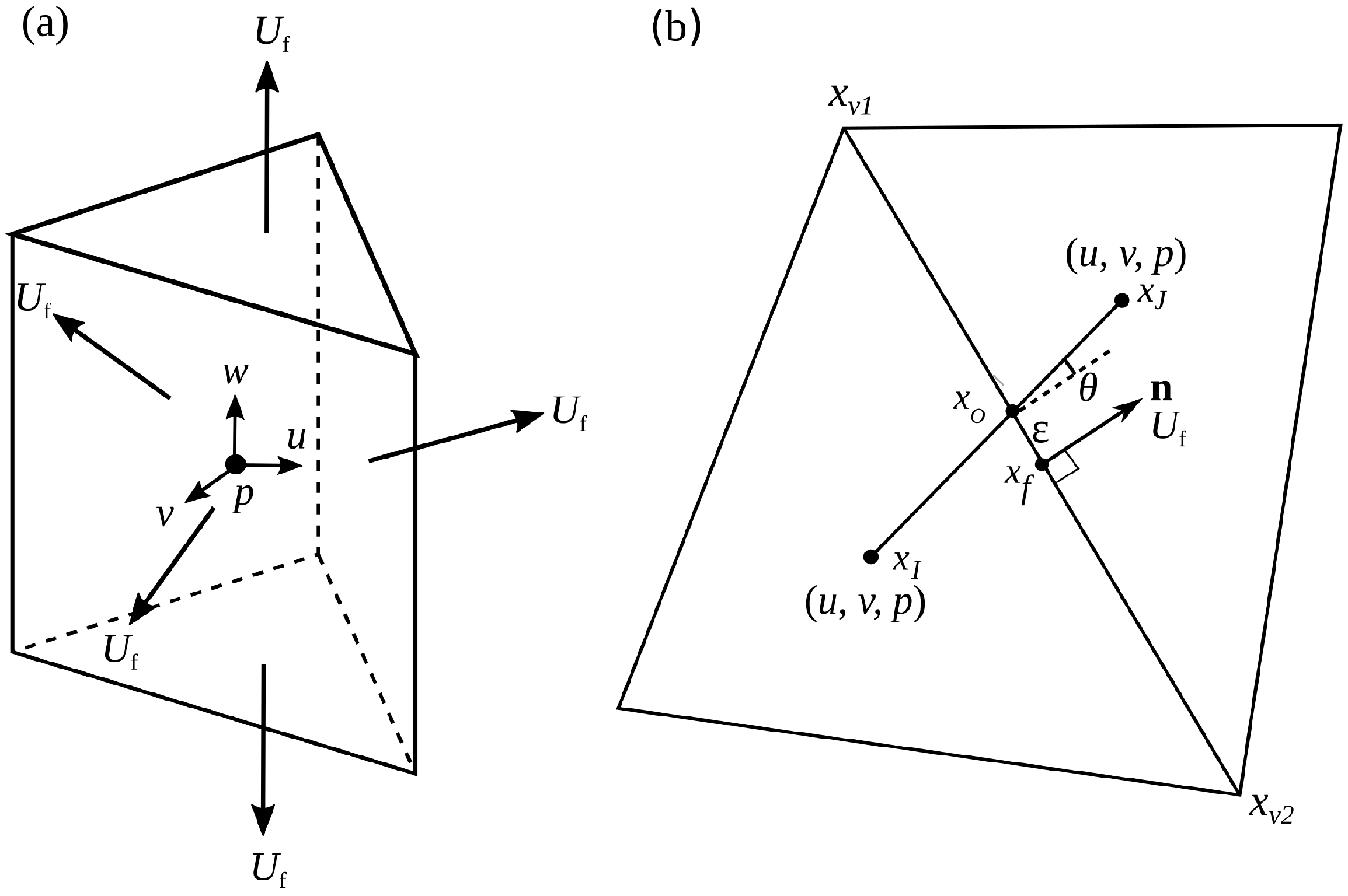
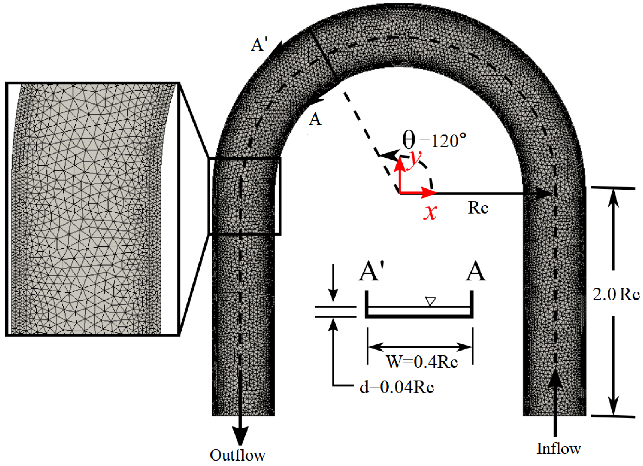
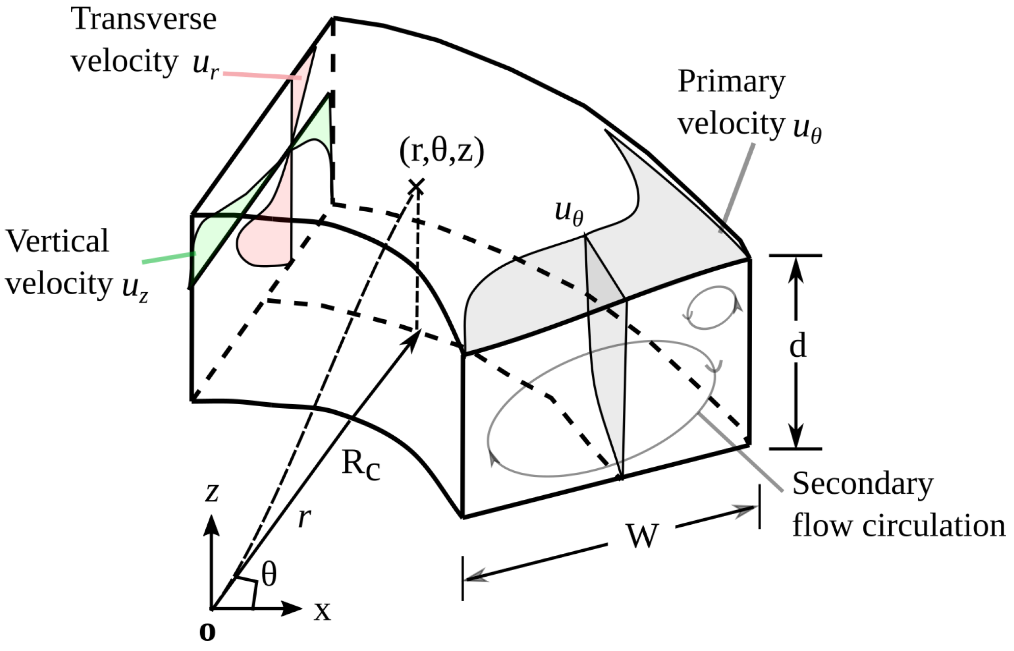
The domain is discretized into triangular prism cells, as shown in Figure 1a. A well-known issue of using traditional non-staggered unstructured grids is that unrealistic pressure oscillations may arise due to the pressure–velocity coupling. This is because all the velocity components $\mathbf{u}$ and pressure p are defined at the cell-centers. In this paper, the momentum interpolation method proposed by Kim and Choi [21] is adopted to avoid oscillation. This method defines a face-normal velocity at the center of each cell face as:

$$U_f={\mathbf{u}}_f·\mathbf{n},$$

(4)

and it is also simple to implement, especially for 3D flows. Here, ${\mathbf{u}}_f$ and $\mathbf{n}$ represent the velocity and outward-normal unit vector at the center on each face of the control volume, respectively.

If the pressure field is hydrostatic, $\partial p_h/\partial z=-\rho g$. There is no need to solve the momentum equation in the vertical direction. The horizontal velocities are solved in the momentum Equation (2), which is explicitly approximated as the following:

$$\frac{{\mathbf{u}}^{n+1}-{\mathbf{u}}^n}{\Delta t}=-\nabla ·\left({\mathbf{u}}^n{\mathbf{u}}^n\right)+\frac{1}{Re}{\nabla }^2{\mathbf{u}}^n,$$

(5)

where superscript n represents time at $t^n$, and $\Delta t$ is the time step.

The vertical velocity is calculated by the continuity equation as $w_{k+1}=w_k-{\nabla }_H{\left(U\Delta z\right)}_k$, where k is the vertical water layer [5]. In addition, it starts with $w_1=0$ at the lower boundary layer. The free surface elevation is obtained from the depth-integral continuity Equation (3). The updated velocity is calculated by $U_f^{n+1}={\mathbf{u}}_f^{n+1}·\mathbf{n}$. The calculation of the face-normal variables are extra work in hydrostatic cases.

For the time-advancement scheme, we consider a second-order Adams–Bashforth method, which is successfully applied to a variety of incompressible flows. The numerical stability of the present formulation is limited by the explicit discretization of the convection and diffusion terms. The Courant–Friedrichs–Lewy (CFL) number is specified according to the original definition given by Kim and Choi [21] as follows:

$$\mathrm{CFL}=\frac{\Delta t}{2}{\oint }_S\left|U\right|dS.$$

(6)

In this work, the numerical simulations are performed by the in-house FORTRAN 90 code NSMP3D. We use the solver SOR, previously shown by [22], with relaxation parameter as $1.0$ and tolerance as ${10}^{-5}$. The numerical discretization in the code is given in the next section.

4. Numerical Discretization

This section will introduce the discretization of N-S equations on the unstructured prism grids, including the integral form of the equations and interpolation of face-normal velocities.

4.1. Integral Form of Equations

A second-order unstructured finite-volume method is chosen to discretize the momentum Equation (5) in each triangular prism V. The governing equations are integrated over a control volume V. The integral form is given by:

$${\int }_V\left(-\nabla ·\left(\mathbf{u}\mathbf{u}\right)+\frac{1}{Re}{\nabla }^2\mathbf{u}\right)dV={\oint }_S\left(-u_i{U}_f+\frac{1}{Re}\frac{\partial u_i}{\partial \mathbf{n}}\right)dS,$$

(7)

where S denotes the cell face.

4.2. Integral Approximation of the Momentum Equation

In integrating the N-S equations over a control volume, we did not introduce any approximation in space. Here, the mid-point rule integral approximation is applied at five faces ($k=1,5$) in the prism-shaped volume. Thus, a second-order accuracy of the cell-centered velocities is obtained, given by:

$${\mathbf{u}}^{n+1}\approx {\mathbf{u}}^n+\frac{\Delta t}{m_V}\sum _{k=1}^5{m}_{S_k}{\left(-{\mathbf{u}}_f^n{U}_f^n+\frac{1}{Re}{\frac{\partial {\mathbf{u}}^n}{\partial \mathbf{n}}}_f\right)}_k,$$

(8)

where $S_k$ represents the face of the prism volume, $m_V$ is the control volume, and $m_S$ is the face area.

The divergence of the velocity is approximated using the interpolation of the known cell-centered velocities ${\mathbf{u}}_f^{*}$ by:

$${\int }_V\frac{\partial {\mathbf{u}}^n}{\partial x_i}dV\approx \sum _{k=1}^5{m}_{S_k}{({\mathbf{u}}_f^n·\mathbf{n})}_k.$$

(9)

4.3. Interpolation of Face-Normal Velocities

The face-normal variables, including velocities, velocity derivatives, and pressure as shown Figure 1b are interpolated from neighboring cell-centers and vertices. ${\mathbf{x}}_I$ and ${\mathbf{x}}_J$ are the cell-centers of the two neighbor cells, ${\mathbf{x}}_O$ is the intersection between the shared face and the cell-centers-overgoing line, and ${\mathbf{x}}_f$ is the center on each face. In this paper, any flow variable at the center of the cell face ${\varphi }_f$ is obtained using a second-order upwind interpolation scheme as follows:

$${\varphi }_f=\left\{\begin{array}{cc}{\varphi }_I+{\psi }_I\nabla {\varphi }_I·({\mathbf{x}}_f-{\mathbf{x}}_I),\hfill & U_f\ge 0,\hfill \\ {\varphi }_J+{\psi }_J\nabla {\varphi }_J·({\mathbf{x}}_f-{\mathbf{x}}_J),\hfill & U_f<0,\hfill \end{array}\right.$$

(10)

where flux limiters ${\psi }_I$ and ${\psi }_J$ are introduced to eliminate non-desirable oscillations using the Local Extremum Diminishing (LED) technique, as described in Vidović et al. [23]. The gradient $\nabla {\varphi }_I$ and $\nabla {\varphi }_J$ at the cell-center is calculated using the Least Squares Method (LSM), presented by Davidson [24].

The outward-normal derivatives in Equation (8) are approximated as proposed by Xue and Barton [25] for high skewness grids:

$${\frac{\partial \varphi }{\partial \mathbf{n}}}_f=\frac{({\varphi }_J+\nabla {\varphi }_J·\epsilon )-({\varphi }_I+\nabla {\varphi }_I·\epsilon )}{{\delta }_{IJ}}+\frac{{\varphi }_{{\mathrm{v}}_2}-{\varphi }_{{\mathrm{v}}_1}}{{\delta }_{{\mathrm{v}}_1{\mathrm{v}}_2}}tan\left(\theta \right),$$

(11)

where ${\delta }_{IJ}$ is the normal distances between ${\mathbf{x}}_I$ and ${\mathbf{x}}_J$; ${\delta }_{{\mathrm{v}}_1{\mathrm{v}}_2}$ is the distance between the vertex ${\mathbf{x}}_{{\mathrm{v}}_1}$ and ${\mathbf{x}}_{{\mathrm{v}}_2}$; $(\epsilon ={\mathbf{x}}_O-{\mathbf{x}}_f)$; and $\theta$ is the angle between Line ${\mathbf{x}}_I-{\mathbf{x}}_J$ and the normal vector $\mathbf{n}$. The distance-weighted averaged value ${\varphi }_{\mathrm{v}}$ is given by:

$${\varphi }_{\mathrm{v}}=\frac{\sum _m{\varphi }_m/L_m}{\sum _{m}1/L_m},$$

(12)

where $L_m$ is the distance between the vertex and the mth neighboring cell-center.

5. Divergence Noise Analysis

The divergence operator, $\mathrm{div}\left({\mathbf{u}}_H\right)$, applies the Gauss theorem on each triangular control volume to approximate the spatially averaged divergence over that cell. It is usually involved in the discretization of the Navier–Stokes (N-S) equation to achieve mass conservation. Take a horizontal generic vector field, ${\mathbf{u}}_H$, in triangular grids, for example. The cell average operator and discrete divergence operator over a cell A are as follows:

$${\overline{\nabla ·\mathbf{u}}}_H=\frac{1}{m_A}{\int }_A\left(\frac{\partial u}{\partial x}+\frac{\partial v}{\partial y}\right)dS=\frac{1}{m_A}\sum _{k=1}^3{\left[{\int }_L\left(u_i{n}_i\right)dl\right]}_k,$$

(13)

and

$$\mathrm{div}\left({\mathbf{u}}_H\right)=\frac{1}{m_A}\sum _{k=1}^3{[\Delta l{\left(u_i\right)}_f{n}_i]}_k=\frac{1}{m_A}\sum _{k=1}^3{(\Delta l{U}_f)}_k,$$

(14)

respectively, where $m_A$ stands for the cell area and $\Delta l$ is the length of the cell edge L.

Let us consider an equilateral triangular grid, for example. The truncation error on this kind of grid shows the checkerboard error patterns of the divergence operator ($\Delta l=\Delta x$) as presented by Wan et al. [3]:

$$\mathrm{div}\left({\mathbf{u}}_H\right)={\overline{\nabla ·\mathbf{u}}}_H+{(-1)}^{\delta }\Delta lH{\left(v\right)}_c-\frac{\Delta l^2}{96}{\left({\nabla }^2(\nabla ·{\mathbf{u}}_H)\right)}_c+O(\Delta l^3),$$

(15)

where the subscript ${\left(\right)}_c$ represents the variable in the cell center, $\delta$ is assigned to each triangle cell to denote its orientation, with 0 and 1 for upward- and downward-pointing triangles, respectively. The functions H reads:

$$H\left(v\right)={\displaystyle \frac{\sqrt{3}}{24}}\left(2{\displaystyle \frac{{\partial }^{2}u}{\partial x\partial y}}+{\displaystyle \frac{{\partial }^{2}v}{\partial x^2}}-{\displaystyle \frac{{\partial }^{2}v}{\partial y^2}}\right).$$

(16)

It can be seen from Equation (15), $\mathrm{div}\left({\mathbf{u}}_H\right)$ is a first-order approximation of both ${\overline{\nabla ·\mathbf{u}}}_H$ and ${(\nabla ·{\mathbf{u}}_H)}_c$. The first-order error term presents the approximation of the cell average in an equilateral triangle. Furthermore, it can be seen from the second term that the sign changes from an upward-pointing triangle to a downward-pointing one, which results in a so-called checkerboard error pattern.

5.1. Divergence Noise Control and Implementation

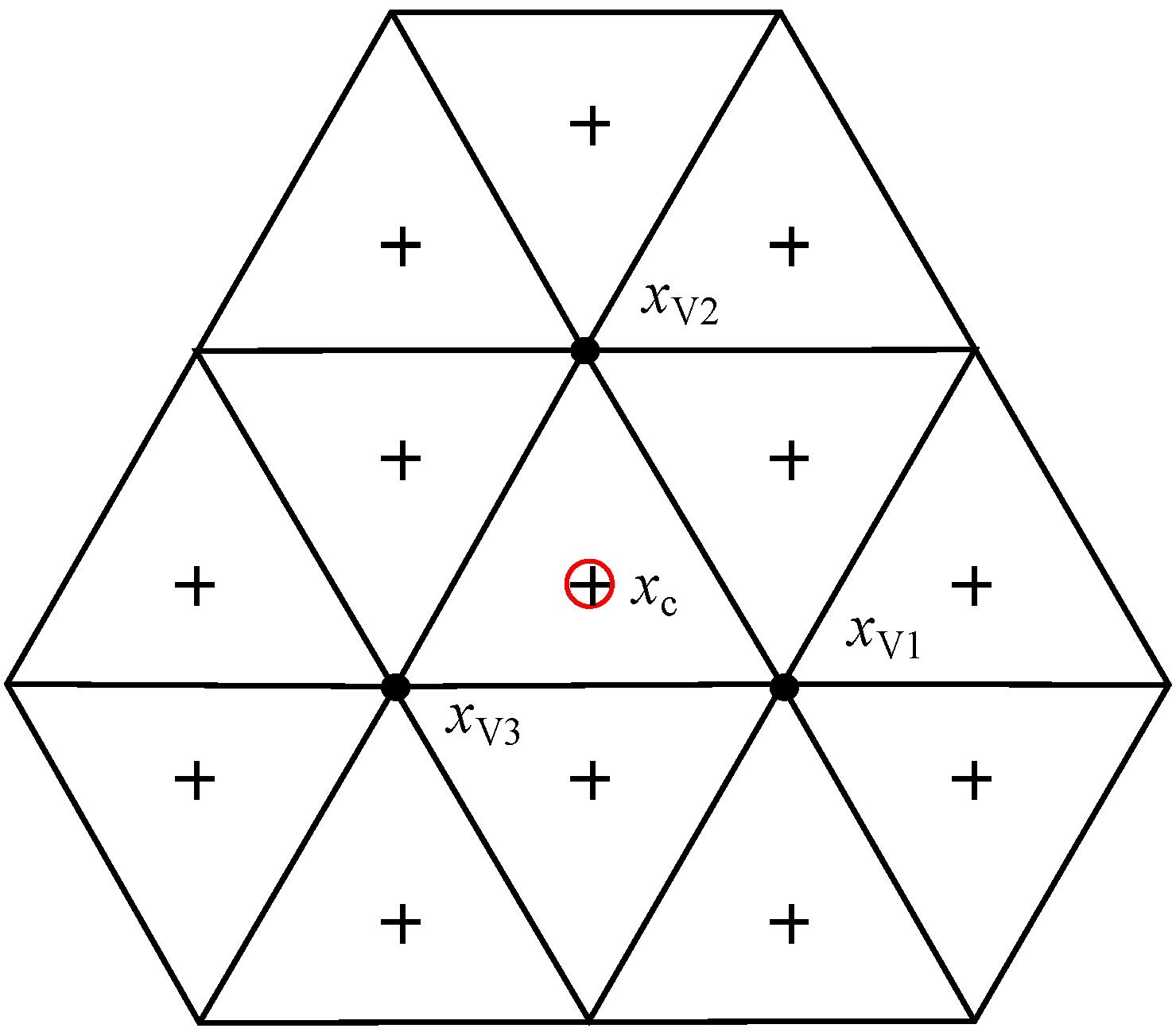
The divergence noise can be eliminated by applying filtered operations [2]. In this work, we improve the performance of the estimation of the divergence operator by using three vertex values in a cell:

$$\mathcal{F}\left[\mathrm{div}\left({\mathbf{u}}_H\right)\right]\left({\mathrm{x}}_c\right)=\frac{1}{3}\sum _{j=1}^3\mathrm{div}\left({\mathbf{u}}_H\right)\left({\mathbf{x}}_{\mathrm{v}j}\right),$$

(17)

where $\mathrm{div}\left({\mathbf{u}}_H\right)\left({\mathbf{x}}_{\mathrm{v}j}\right)$ in the vertex is calculated by Equation (12). This is, in a sense, equivalent to a Shapiro first-order implicit nodal filter proposed by Wolfram and Fringer [2] using node downsampling and upsampling. In equilateral grids, the filter stencil is enlarged to all cells sharing a vertex, including 13 cell-centers, see Figure 2. The pressure and velocity components are calculated separately in the proposed hydrostatic formulation. Vertical velocities are calculated from horizontal divergences, resulting in divergence errors and further influence elevation, similar to the classic staggered approach [5,26].

In the proposed hydrostatic formulation, the pressure and the velocity components are calculated separately. Vertical velocities are calculated from horizontal divergences, resulting in divergence errors and further influence elevation, similar to the classic staggered approach [5,26]. To better understand the divergence in solving the N-S equation steps and to implement the filtered technique,

Table 2. The diagram of divergence, $\mathrm{div}\left(\mathbf{u}\right)$, sequence in hydrostatic calculations.

Hydrostatic Calculations
(0) $U_f^n={\mathbf{u}}_f^n·\mathbf{n}$;
(1) Calculate ${\mathbf{u}}^{n+1}$ and ${\mathrm{v}}^{n+1}$ based on $U_f^n$; Calculate $U_f^{n+1}={\mathbf{u}}_f^{n+1}·\mathbf{n}$;
(2) Calculate $\mathrm{div}\left({\mathbf{u}}_H^{n+1}\right)$ based on $U_f^{n+1}$;
(3) $w_{k+1}^{n+1}$ based on $w_k^{n+1}$ and $\mathrm{div}\left({\mathbf{u}}_H^{n+1}\right);$ ${\eta }^{n+1}$ based on $\mathrm{div}\left({\mathbf{u}}_H^{n+1}\right)$
(4) $p_h^{n+1}=\rho g({\eta }^{n+1}-z)$ and go to step 1

summarizes the steps concerning the hydrostatic calculations involved with a free surface. They follow the divergence $\mathrm{div}\left(\mathbf{u}\right)$ displayed in the order in the program.

5.2. An Example of the Divergence Noise Control

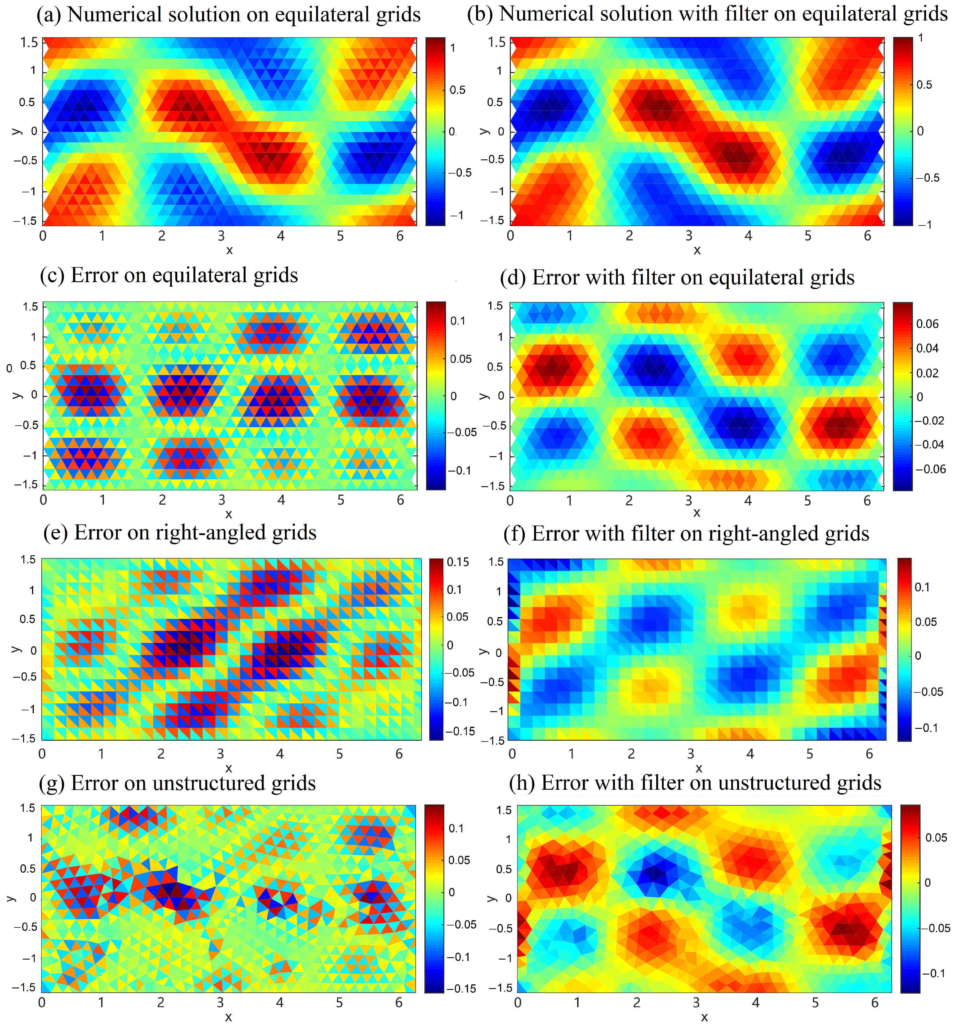
The following is an example to show the truncation error pattern with or without the filtered technique. The order and checker-board behavior are studied by the vector field

$$\mathbf{u}=\frac{1}{2\sqrt{2\pi }}\left(\frac{\sqrt{105}}{2}cos\left(2x\right){cos}^2\left(y\right)sin\left(y\right),-\sqrt{15}cos\left(x\right)cos\left(y\right)sin\left(y\right)\right),$$

and the analytical divergence solution

$$\nabla ·\mathbf{u}=-\frac{1}{2\sqrt{2\pi }}\left(\sqrt{105}sin\left(2x\right){cos}^2\left(y\right)sin\left(y\right)+\sqrt{15}cos\left(x\right)cos\left(2y\right)\right),$$

over the computational domain $[0,2\pi ]\times [-\frac{\pi }{2},\frac{\pi }{2}]$. The discrete divergence, $\mathrm{div}\left({\mathbf{u}}_H\right)$, is gained by applying the divergence operator (14). The numerical solution is compared with the cell-centers’ divergence, ${(\nabla ·\mathbf{u})}_c$ with grid resolution $\Delta x=0.2$. The numerical error, shown in Figure 3a,c, confirms that the divergence operator yields a first-order checkerboard error pattern, as presented by Wan et al. [3]. 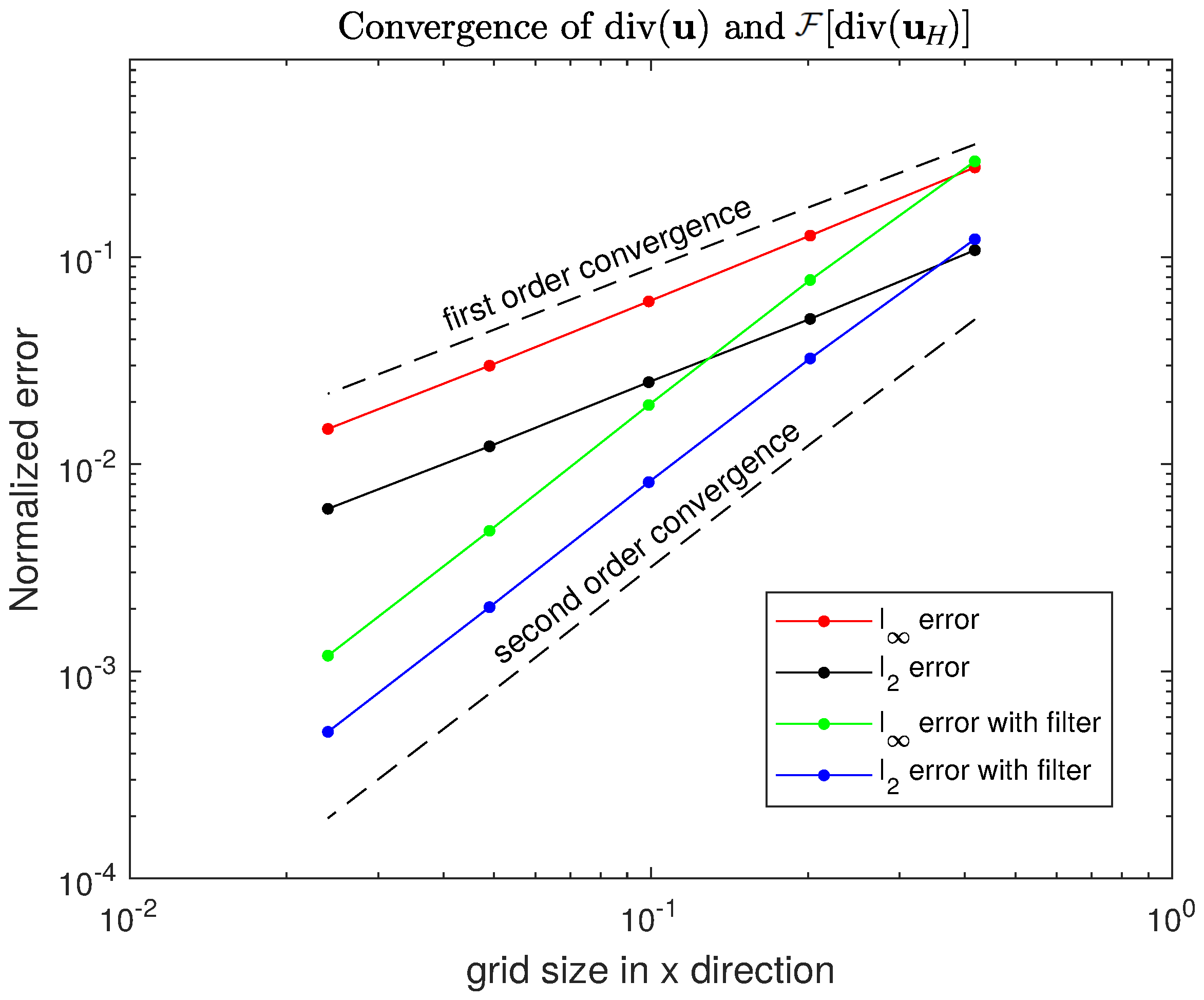Figure 3b,d present the numerical solution and errors using the filtered scheme. The numerical error is computed concerning the cell average. Clearly, the checkerboard errors are already eliminated. In addition, the method now shows a second-order accuracy as in Figure 4.

The checker-board errors before and after the filtered scheme (17) in the right-angled grids case are shown in Figure 3e,f, respectively. The divergence noise is mitigated after filtering. Figure 3g presents a similar checkerboard pattern for fully unstructured grids as the equilateral case. Moreover, as Figure 3h shows, the filtered scheme (17) eliminates the error even for unstructured grids. The largest errors are noticed close to the boundary, which is expected because fewer neighbor cells are available for the vertex calculation.

6. Numerical Results

Flows in the curved channel calculated by hydrostatic pressure are selected to illustrate our model. The geometry and profile of the primary and secondary flows in the axisymmetric curved channel are shown in Figure 5. In the streamwise direction, the non-dimensional coordinate and velocity are $\theta$ and $u_{\theta }$, respectively. In the spanwise direction, the transverse and vertical velocities $u_r$ and $u_z$ correspond to the r and z directions, composing the secondary circulations.

The physical problem can be described in terms of four-dimensional numbers: W, d, $R_c$, and U. Water depth d is chosen to be the scale L in the non-dimensional equations. Thus, the above dimensional variables can be uniquely prescribed in terms of the Reynolds number $Re=Ud/\nu$, the Deans number $Dn=Re\sqrt{\epsilon }$ with a curvature aspect ratio $\epsilon =d/R_c$, and the aspect ratio $\delta =d/W$. In the following simulations, we compare the present results with the analytical solutions provided by de Vriend [14] with a ${180}^{\circ }$ sharp bend. Parameters $\delta =0.1$, $\epsilon =0.04$, and $Dn=25$ corresponding to $Re=125$ are chosen in this paper. All quantities hereafter are in non-dimensional units (star notation is omitted for clarity).

It is also necessary to set our results in cylindrical coordinates ($\theta ,r$), for which the transformation is given by:

$$u_{\theta }=-usin\theta +vcos\theta ,u_r=ucos\theta +vsin\theta ,$$

(18)

where $(u,v)$ and $(u_{\theta },u_r)$ are the horizontal velocity components in Cartesian and cylindrical coordinates, respectively. Finally, the curved channel flow in the cylindrical coordinate is normalized by:

$$u_{\theta }=V{\tilde{u}}_{\theta },u_r=\epsilon V{\tilde{u}}_r,u_z=\epsilon V{\tilde{u}}_z,$$

(19)

where V is the velocity scale, $\epsilon$ is the curvature aspect ratio, and $({\tilde{u}}_r,{\tilde{u}}_{\theta },{\tilde{u}}_z)$ represents the non-dimensional velocity for the direct framework, as in Figure 5.

The horizontal triangular grid is shown in Figure 6. $A-A^{{}^{\prime }}$ ($\theta ={120}^{\circ }$) is selected as a typical section to compare with analytical solutions from de Vriend [14]. A total of 32 layers are used because w is iterated explicitly from the bottom to the top. There are a total of 602,016 cells, which is more than the 528,260 in Wolfram and Fringer [2]. To precisely show the secondary velocities with rapid change close to the channel wall in the transverse direction, grids are set finer close to the wall boundary with $\Delta r_{\min }=0.2d$ and $\Delta r_{\max }=0.6d$, as $d=L$ is used for scale. The non-dimensional value is $U_{\max }\Delta t/\Delta r_{\min }=0.24$, which is smaller than 1.

The boundary conditions are also shown in Figure 6, a prescribed inflow velocity and zero-pressure at the outflow with sufficiently long inlets and outlets are set to allow the full development of flow in the curved channel. The kinematic free surface condition is used. The elevation is set as the Neumann boundary in the inlet and set to be zero in the outlet.

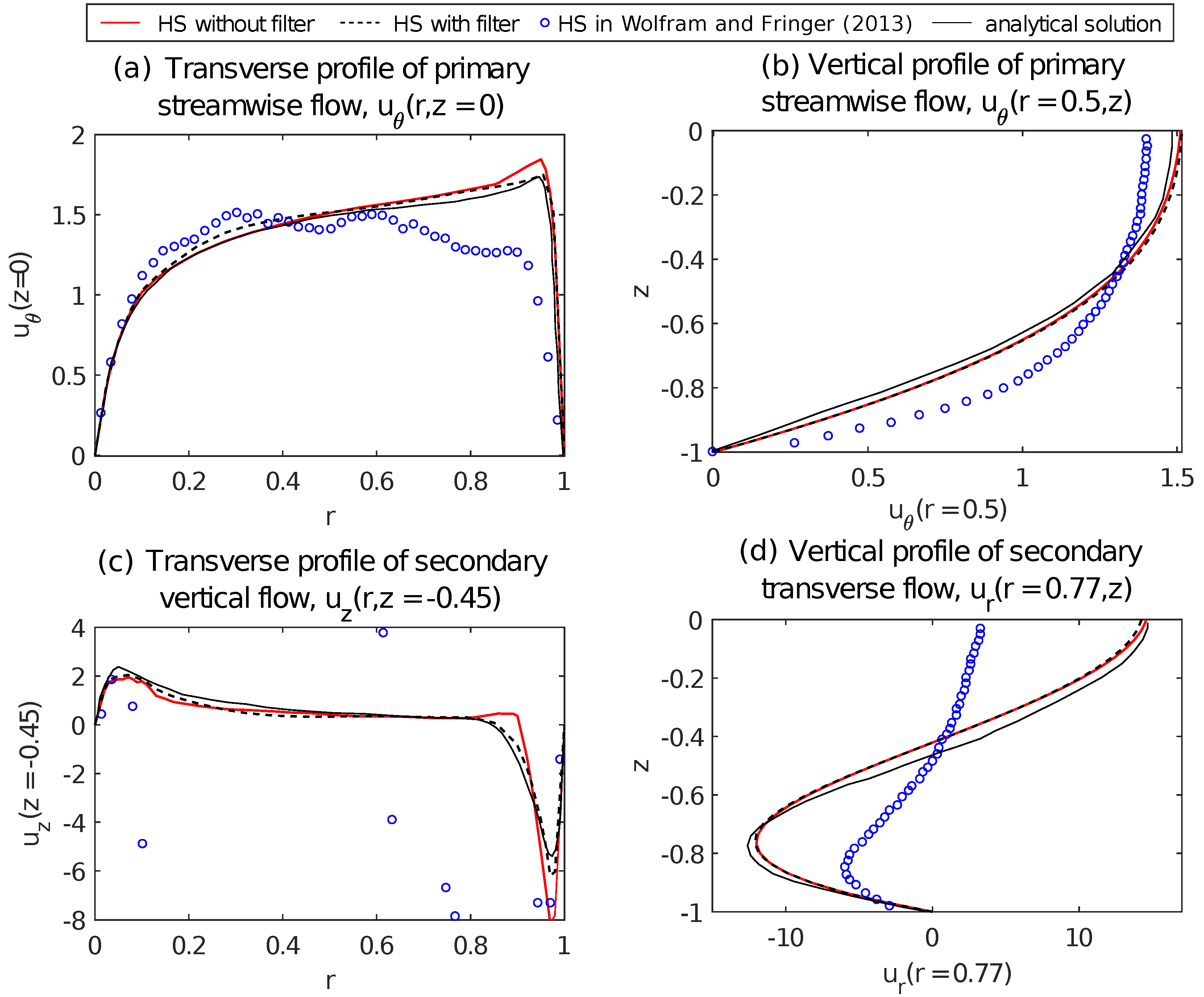
6.1. Velocity Profiles

To validate our results, we compare the velocity profiles with the analytical solutions from de Vriend [14] and the numerical model from Wolfram and Fringer [2]. Note that four flow profiles are close to the analytical results for calculations with filter scheme, as shown in Figure 7. The absence of the filtered technique results in a solution with reduced precision. However, the results are still close to the analytical solution. As expected, the filtered technique improves the numerical solution. It is worth noting that the proposed method with or without the filter gives more accurate results than the ones by Wolfram and Fringer [2]. There are considerable oscillations and even an opposite peak velocity at the outer border if the filtered method was not applied in Wolfram and Fringer [2], so they concluded that filtering is important for hydrostatic calculations with rigid surfaces. Our simulations have no significant oscillations, even for non-filtered hydrostatic calculations with the free surface. Furthermore, whether a filter is applied does not change the peak qualitatively, and the peak sign is the same as the analytical solution.

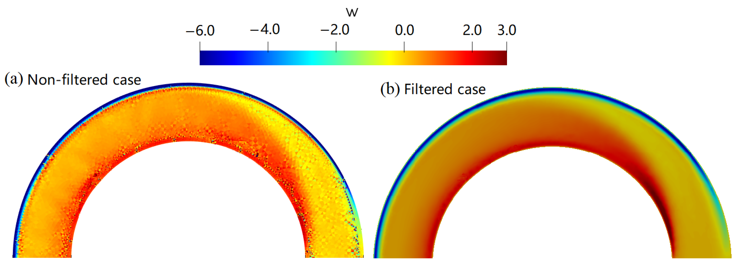
Figure 8 illustrates a two-dimensional view of the vertical velocity $w(r,\theta ,z=-0.5)$ for the different formulations presented in this paper. The results are smooth for filtered calculations. However, for non-filtered approximation, the vertical velocity has some oscillations. This behavior indicates that although it is not necessary, the filtered method is highly recommended in hydrostatic calculations.

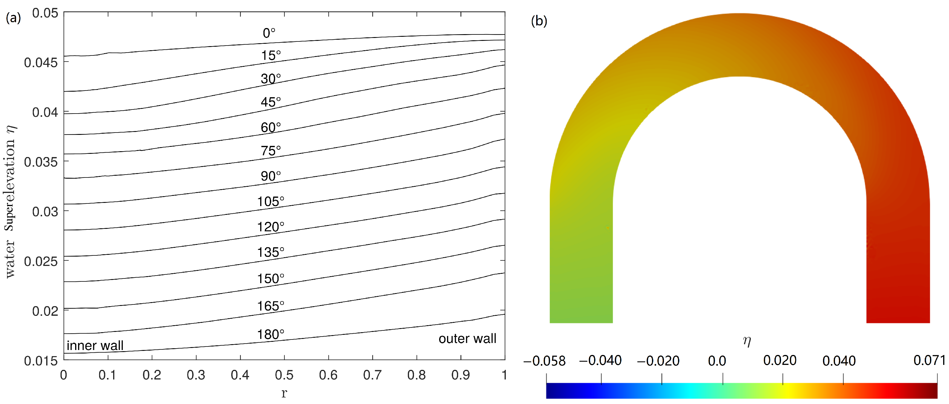
6.2. Water Surface Elevations

This section further analyzes the filtered method by presenting the water surface approximation. The water surface slope points from the outer (concave) bank to the inner (convex) bank in the curved channel due to the centrifugal force. The transversal water slope will increase with the primary flow velocity and the inverse radius of curvature. At the bend entrance $(\theta =0^{\circ })$, the water surface forms a lateral slope, and the maximum lateral slope appears at the section slightly upstream of the mid-point of the bend $(\theta ={90}^{\circ })$. The superelevation refers to the height difference of the lateral water surface. The classical relationship between the superelevation and the Froude number is first proposed by Ippen [12] as:

$$\Delta h\propto F{r}^2,$$

(20)

where $\Delta h$ is the superelevation. The increasing Froude number will raise the superelevation.

Figure 9a displays the transverse surface elevation across different channel sections. It can be seen that superelevation is mainly distributed at the outer bank, and the depression is near the inner bank, as expected. The water superelevation at $0^{\circ }$, ${90}^{\circ }$, and ${180}^{\circ }$ channel cross-sections are $0.002$, $0.004$, and $0.0025$, respectively. The surface increases suddenly from $0^{\circ }$ to ${15}^{\circ }$ when the water begins to come into the curved part. Symmetrically, the surface decreased suddenly from ${165}^{\circ }$ to ${180}^{\circ }$ when the water goes outside of the curved part. This phenomenon is similar to the results from Drinker [27]. Figure 9b shows the water surface elevation for $Fr=0.1$. The elevation decreases along the longitudinal direction. Simultaneously, the elevation in the outer part is higher than that in the inner part. The lateral superelevation is independent of the radial distribution of the flow velocity.

Table 3. Water superelevations versus Froude numbers ($F{r}_1$ and $\Delta h_1$ correspond to the case: $Fr=0.1$).

$\mathit{Fr}$	${\mathit{\eta }}_{\mathit{inner}}$	${\mathit{\eta }}_{\mathit{outer}}$	$\mathbf{\Delta }\mathit{h}$	${(\mathit{Fr}/{\mathit{Fr}}_1)}^2$	$\mathbf{\Delta }\mathit{h}/\mathbf{\Delta }{\mathit{h}}_1$
0.1	0.0254	0.03175	0.00635	-	-
0.2	0.1290	0.1575	0.0285	4	4.4
0.3	0.4133	0.4800	0.0667	9	10.5
0.4	0.9210	1.0297	0.1087	16	17.1
0.6	2.1498	2.3752	0.2254	36	35.5

presents the water surface elevation for different Froude numbers. We find that when the Froude number increases ${(Fr/F{r}_1)}^2$ times, the superelevation increases $\Delta h/\Delta h_1$ times in our calculations, in agreement with Equation (20). Here, $F{r}_1$ and $\Delta h_1$ correspond to the values of the first line of Table 3.

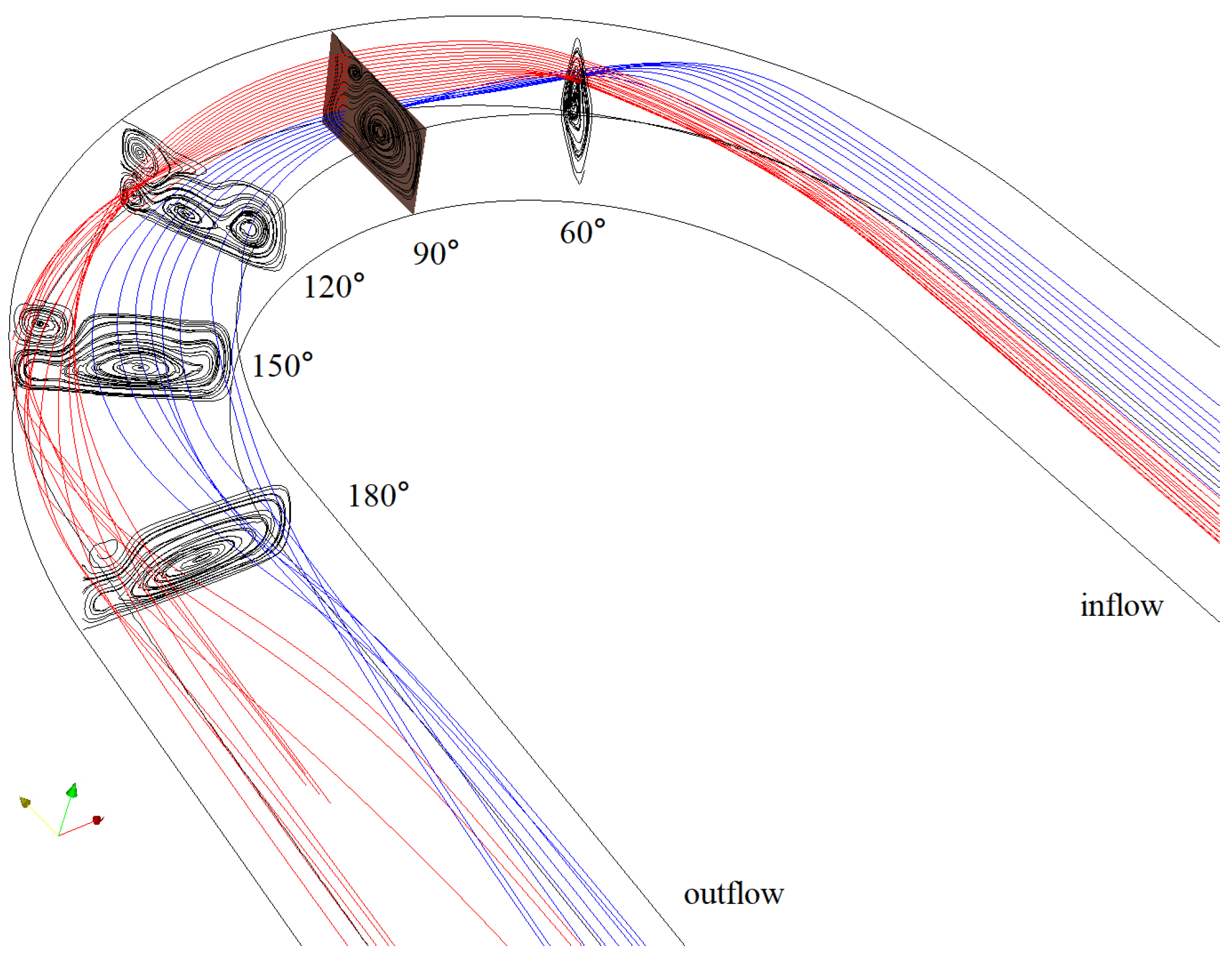
6.3. Secondary Flow Effects

Figure 10 shows the three-dimensional streamlines in the curved channel at $Fr=0.4$. The primary streamlines are chosen at $(x=0;y=28)$, located from the bottom to top at the ${90}^{\circ }$ cross-section with the red line above the blue line. The streamlines mix with red lines to the outer part and blue lines to the bends’ inner part. We can also notice the streamlines change in the five typical cross-sections. Details about the secondary flow results in filtered calculations can be found in Figure 11 and Figure 12. The main transverse flow directs from the outer to the inner bank in the near-bed region and opposite at the free surface. A separate transverse flow directs from the outer to the inner bank at the free surface near the outer part. This will generate a superelevation at the outer bank. Finally, the transverse flow forms secondary flow patterns [28,29]. The simulation results are in full agreement with the mechanisms responsible for the meandering of rivers. The following discusses the secondary flows in detail.

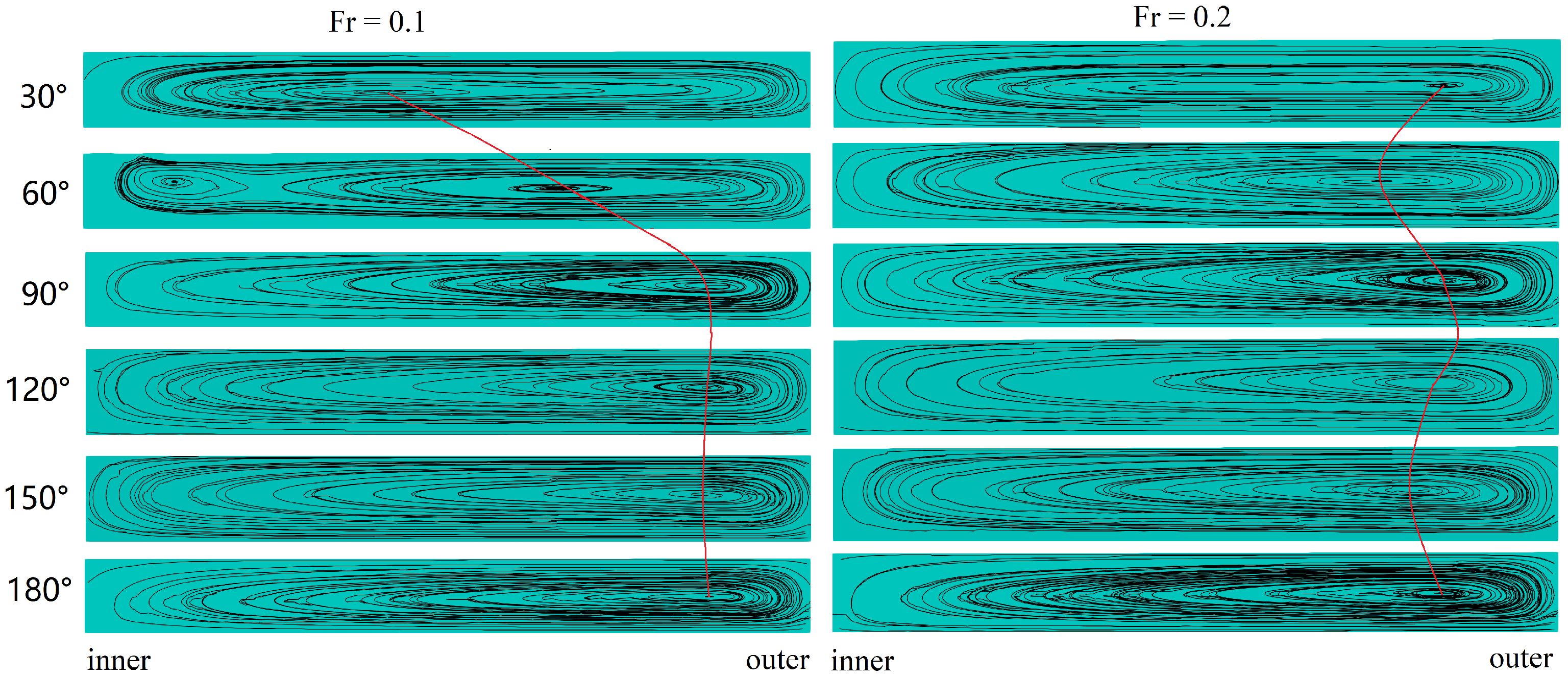
Figure 11 compares the streamlines at six cross-sections between calculations with the free surface at $Fr=0.1$ and $Fr=0.2$. The secondary flow center quickly moves to the outer part of the channel from $0^{\circ }$ to ${90}^{\circ }$ and keeps its position at the convex bank until ${180}^{\circ }$. The primary vortex splits into two in ${60}^{\circ }$, and then the vortex merges to be one until the outflow boundary. The surface elevation is very small, $\Delta \eta /h=0.07$. The track of the vortex core is the same as $Fr=0.1$. With the increase in the Froude numbers up to $Fr=0.3$, the longitudinal elevation increases to be $\Delta \eta /h=0.75$. There is only one primary vortex remaining in all the cross-sections up to $Fr=0.3$. The vortex changes its path compared to cases with smaller Froude numbers. At ${30}^{\circ }$, the core moves close to the outer boundary and slightly moves forward and downward at the convex bank. At ${60}^{\circ }$, the primary vortex does not split into two compared with the cases of smaller Froude numbers. The size of the vortex also increases to adjust the surface elevation.

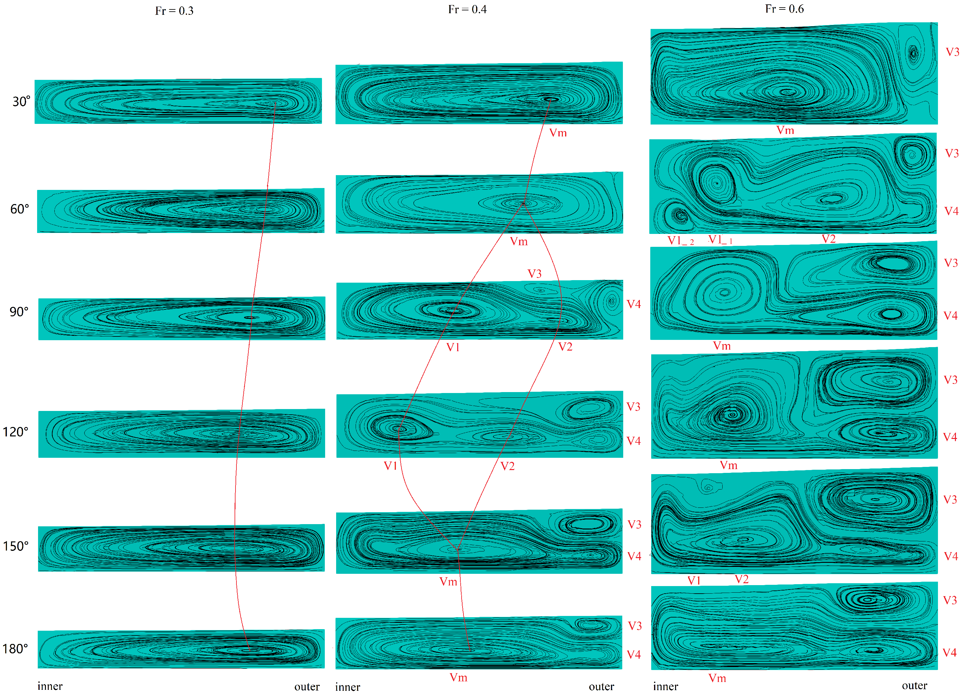
As shown in Figure 12, the vortex number increases when the Froude number is up to $Fr=0.6$. There is only one primary vortex (Vm) when $Fr=0.4$ at ${30}^{\circ }$ and ${60}^{\circ }$. Then, the vortex splits into four vortices (V1, V2, V3, V4) in the ${90}^{\circ }$ and ${120}^{\circ }$ sections. Two vortices (V1, V2) merge to be one vortex (Vm1), occupying most of the section, located in the inner part. At ${90}^{\circ }$, there is a transition section forming the vortex (V3 and V4). They move to the convex bank side by side in the vertical direction. The distribution of the vortex is more complex when $Fr=0.6$. Generally, the vortex pattern is similar to the case $Fr=0.4$. The flow quickly forms two vortices (Vm and V3) at ${30}^{\circ }$ and comes to be the same pattern as $Fr=0.4$ at ${180}^{\circ }$. Between these two sections, in the inner part of the channel, the vortex (Vm) also splits in two (V1 and V2) side by side due to the high water depth. Simultaneously, the lower transverse surface elevation will meet the boundary condition ($\eta =0$) at the outflow. The longitudinal elevations are $\Delta \eta /h=1.4$ and $\Delta \eta /h=3.4$, respectively.

From a mathematical perspective, the changes mentioned earlier in the secondary flow state can be explained by Dean numbers. This is named after Dean, who was the first researcher to confirm the existence of a pair of counter-rotating vortices as secondary circulations in the fully developed curved pipe flow [30]. Here, we have one vortex in the open channel. The Dean number $Dn=Re\sqrt{\epsilon }$ is composed by the Reynolds number and the curvature aspect ratio $\epsilon =d/R_c$. In our simulations, the Reynolds numbers are the same for all cases. Due to the elevation in the longitudinal and transverse direction, the water depth d changes accordingly and influences the curvature aspect ratio $\epsilon$. In another aspect, in the whole channel domain for Case 1 and Case 3, $Dn$ acts accordingly from 25 to 50, which is relatively small. Ligrani et al. [31] and Nivedita et al. [32] also pointed out that when the Dean number exceeds a critical value, a transition from laminar is observed with the development of the secondary flow near the outer wall. This will eventually generate arrays of counter-rotating Dean vortex pairs downstream for closed curved channel flow.

7. Discussion

In this paper, we notice the inaccuracies in the approximation of the divergence operator in solving N-S equations and instabilities due to spurious pressure modes associated with the unstaggered arrangements that show similar behavior as the divergence noise presented by [2] with staggered grids. Therefore, a novel filtered method (Equation (17)) is proposed to avoid these inaccuracies.

In Section 5, the filtered effect is demonstrated by an example with an analytical solution. In the aspect of the filtered effect on different grids, we notice that there will be horizontal divergence noise in both structured equilateral and right-angled grids. Only the error pattern is different. The maximum error from the right-angled grids is even more significant than the unstructured grids. These results conclude that adopting a structured grid will not improve the divergence noise. In the aspect of the divergence operator accuracy, the numerical error analysis confirms that it yields a first-order checkerboard error pattern. After filtering, the errors are eliminated in three different grids. Numerical results show a second-order accuracy after this filtered technique.

In the aspect of the composing effect of the filtered method, hydrostatic pressure, free surface elevation, and secondary flows in the curved channel flow, Section 6 provides the velocities compared with [2]. The velocity profiles in filtered and non-filtered calculations show that the absence of the filtered technique results in an oscillatory vertical velocity with reduced accuracy. Our non-filtered hydrostatic results are, in a sense, better than those by Wolfram and Fringer [2] with an opposite peak, qualitatively. The filtered method is highly recommended in hydrostatic calculations.

Furthermore, with the calculation of this filtered method, we find that there are elevations in both the longitudinal and transverse directions. The surface increases suddenly when the water begins to come into the curved part and decreases suddenly when the water goes outside. The superelevation is proportional to the Froude numbers. The free surface elevations influence the water depth and further affect the secondary flow status. With the increase in the $Fr$ number, the vortex pattern and vortex number are changed in the cross-section of the curved channel, which can be explained by the Dean number [30].

This study focuses on the sharply curved channel with a ${180}^{\circ }$ bend at $Re=125$. Concerning the future work of the present paper, we expect that our work will provide a useful guide for scientists in charge of similar simulations of hydrostatic curved channel flow. As the unstructured mesh is flexible to discrete the domain with arbitrary geometries, we can apply the filtered method to analyze the physical behavior of the curved channel with other curvatures, such as kinoshita curves in [33] and the confluence in [34].

8. Conclusions

This paper proposes a novel three-dimensional hydrostatic method for flows in a curved channel based on an unstructured finite-volume method and a filtering technique with non-staggered triangular grids. First, teh numerical results confirm that a filtered approximation of the divergence operator eliminates the checkerboard error pattern and yields an accurate second-order method. Next, we analyze the method’s performance in terms of the divergence approximation velocity and water elevations for a ${180}^{\circ }$ curved channel. As expected, although the numerical results with or without filtering are close to the analytical solution, the filtered technique significantly improves the numerical solution. Moreover, the present formulation results in more accurate results than those presented by [2]. Numerical results also show that the method correctly approximates the water surface elevations: The superelevation is mainly distributed at the outer bank, the depression is near the inner bank, and the elevations agree with the Ippen formula [12]. For the velocity field, the streamlines change at different cross-sections of the curved channel, and their behavior is directly related to the Froude number. The streamline centers keep the same track when $Fr$ is smaller than $0.1$. However, the path changes when the $Fr$ is up to 0.3, keeping the same number of vortices. When $Fr$ is higher, the water surfaces increase, and the primary vortex splits into four at several cross-sections. Finally, future work will focus on applying the proposed numerical method to analyze curved channels with other curvatures, turbulent flows, and scour development.