
Intensity-Duration-Frequency Curve for Extreme Rainfall Event Characterization, in the High Tropical Andes

 , , , , , , , , and
Abstract
1. Introduction
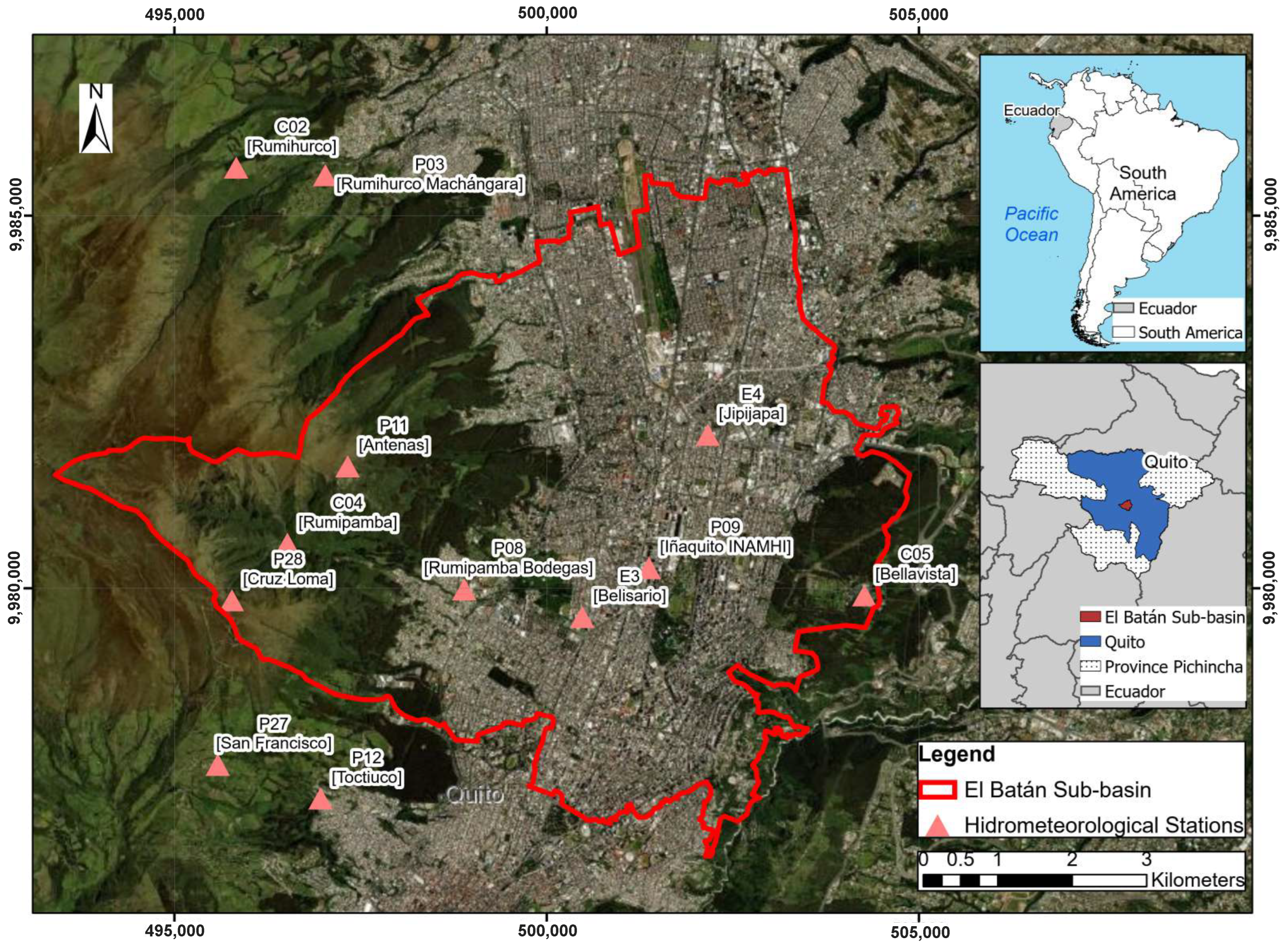
2. Study Area
3. Data
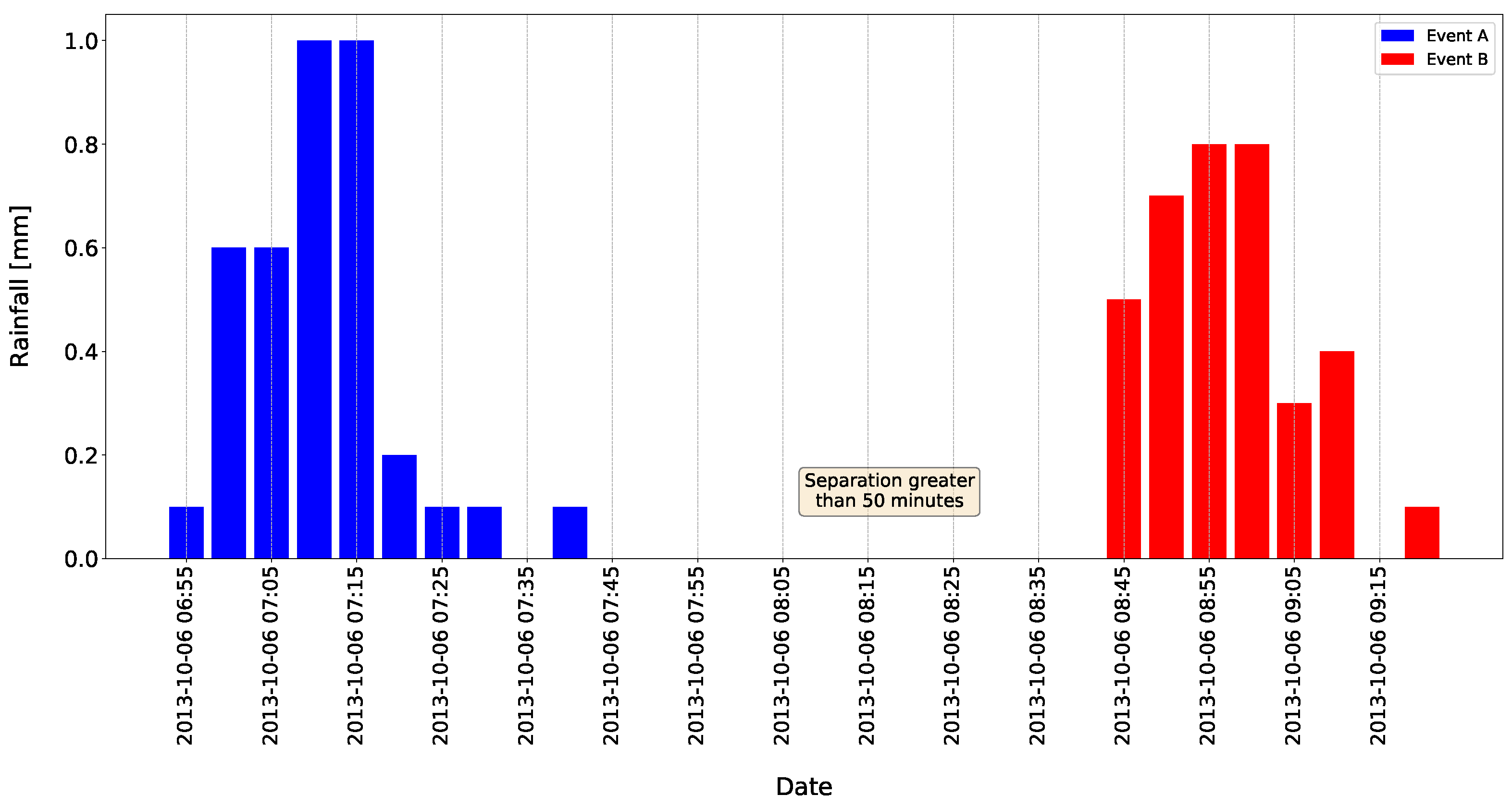
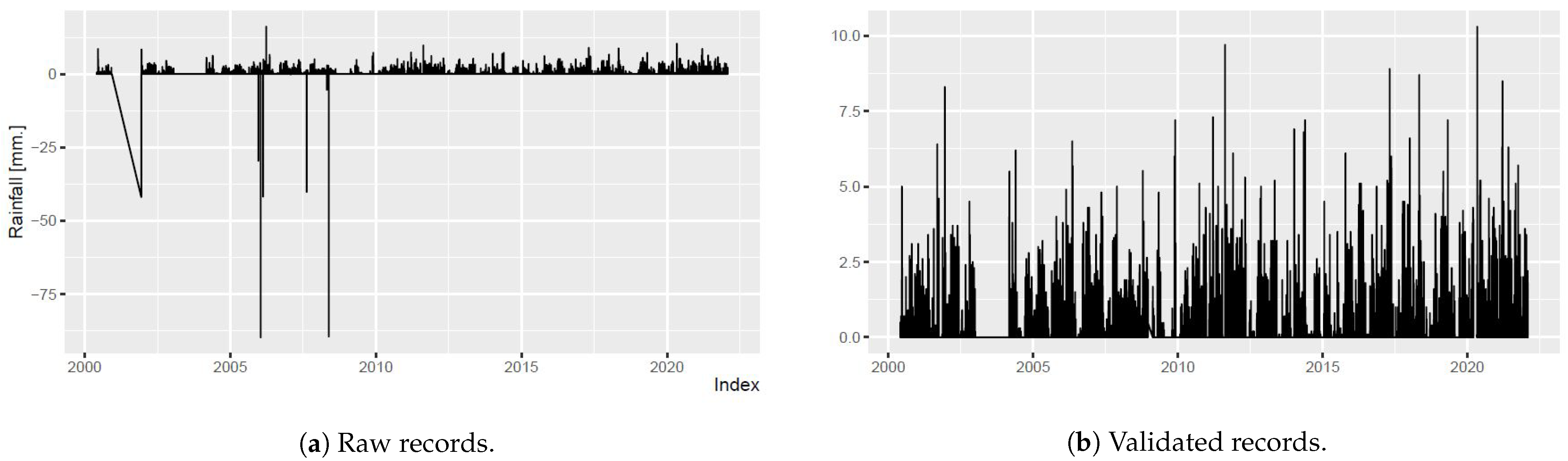
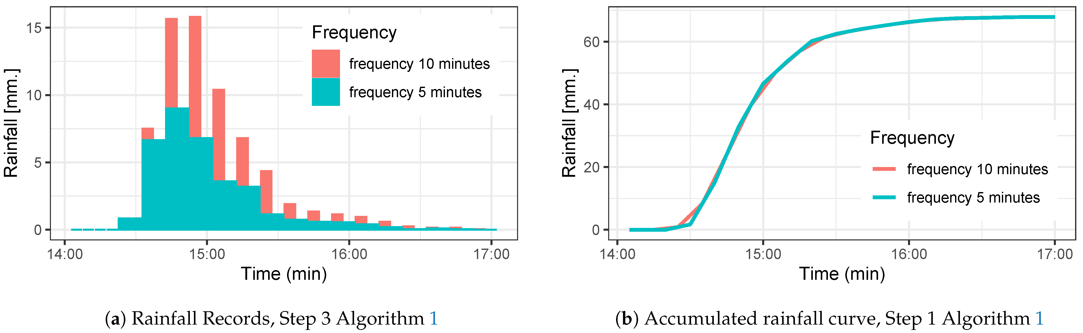
Data Preprocessing
| Algorithm 1: Frequency reduction | |
| 1 | Input:Rainfall time series with frequency of ten minutes. |
| |
| Output: Rainfall time series with a frequency of five minutes. | |
| Algorithm 2: Sliding window algorithm for capturing maximum rainfall events | |
| 1 | Input:Rainfall time series and the desired duration |
| |
| Output: Maximum rainfall events- | |
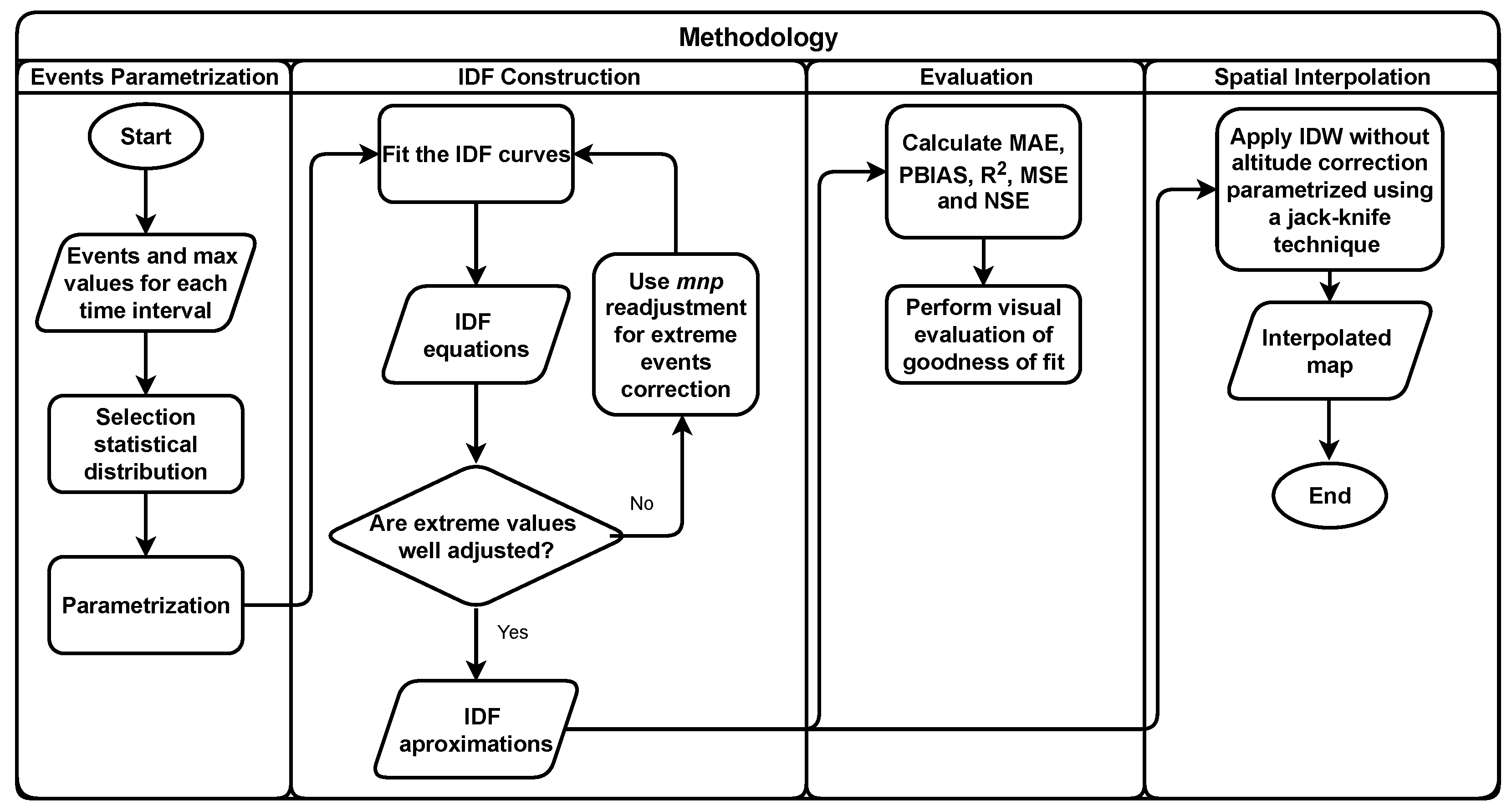
4. Methodology
4.1. Distribution Functions and IDF Curves Construction
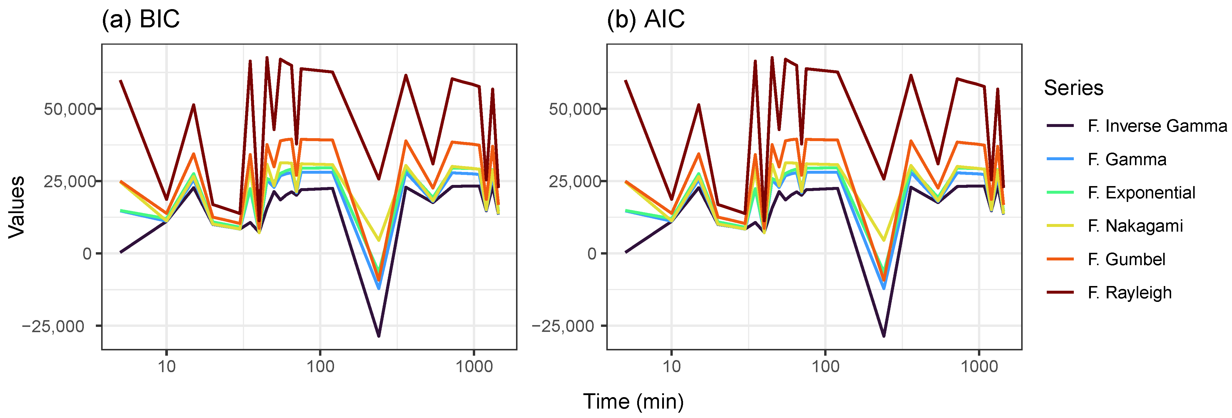
4.1.1. Statistical Distribution Selection and Parametrization
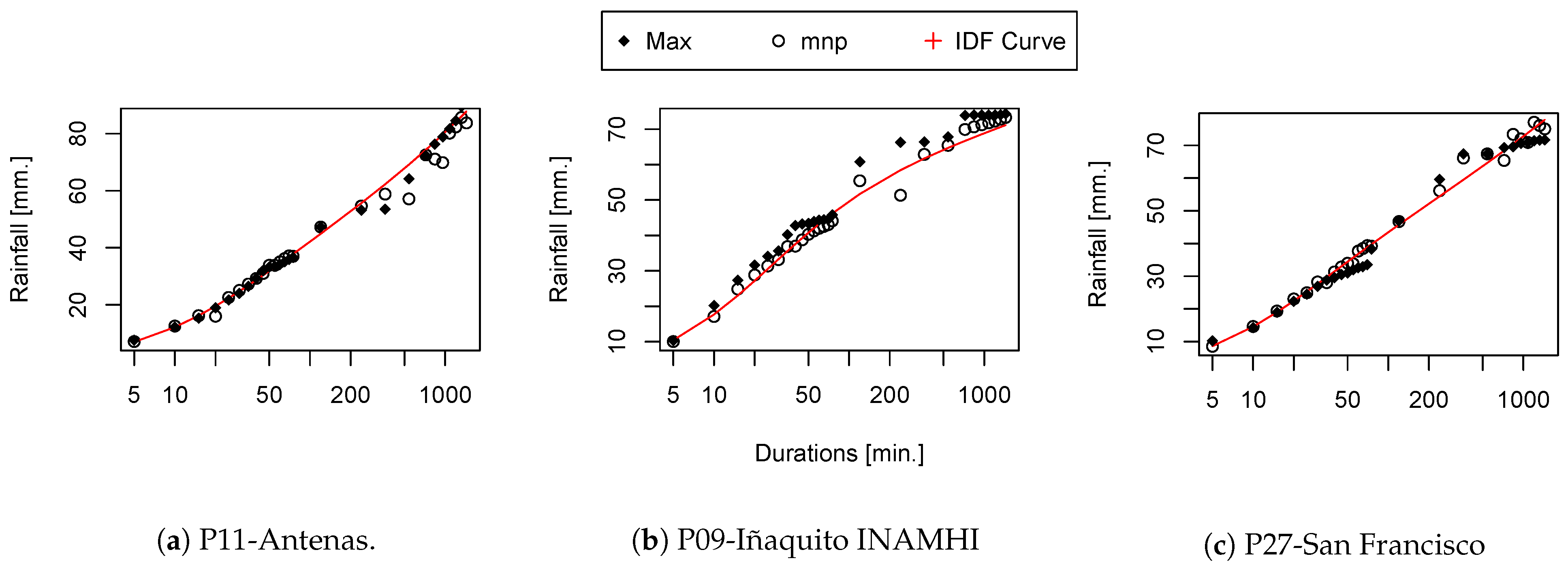
4.1.2. IDF Fit
4.1.3. The mnp Readjustment for Extreme Events Correction
4.2. Evaluation
4.3. Interpolation
5. Results
5.1. Data Preprocessing
5.2. Distribution Functions and IDF Curves Construction
5.2.1. Statistical distribution selection and parametrization
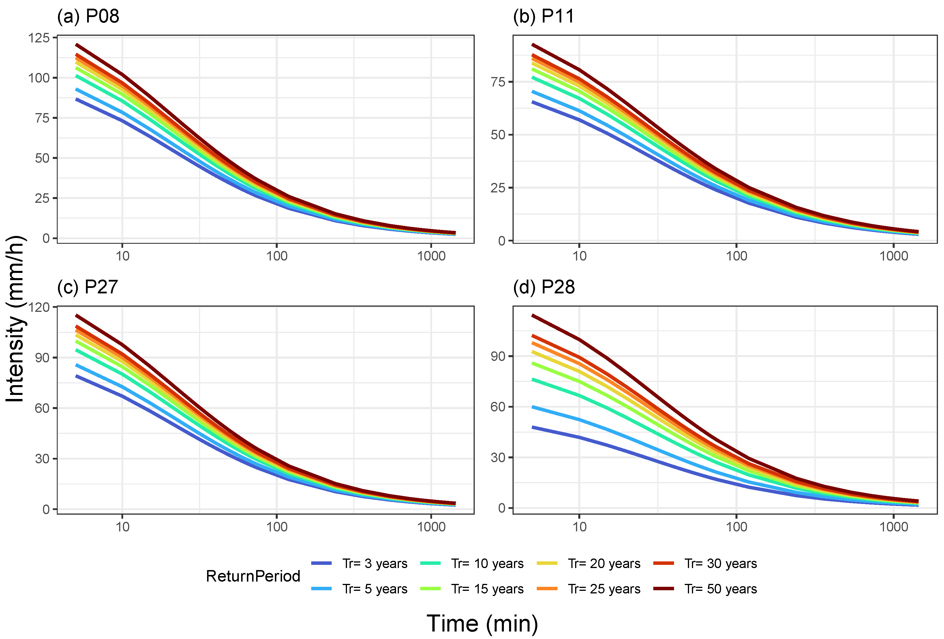
5.2.2. IDF Fit & the mnp Readjustment for Extreme Events Correction
5.3. Evaluation
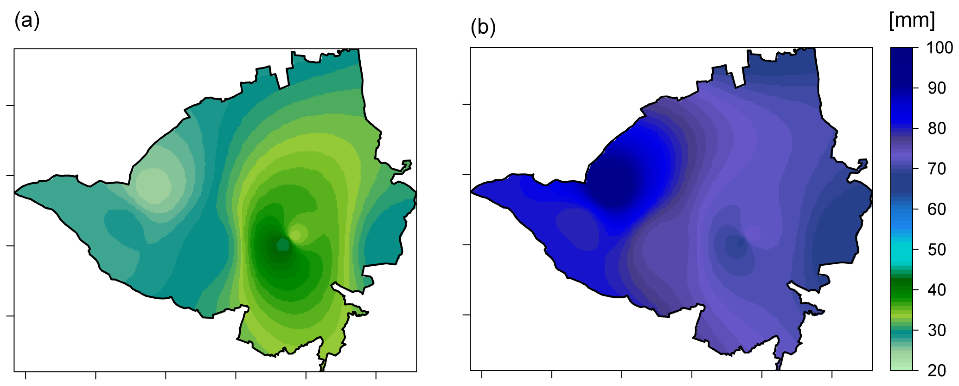
5.4. Spatial Interpolation
6. Discussion
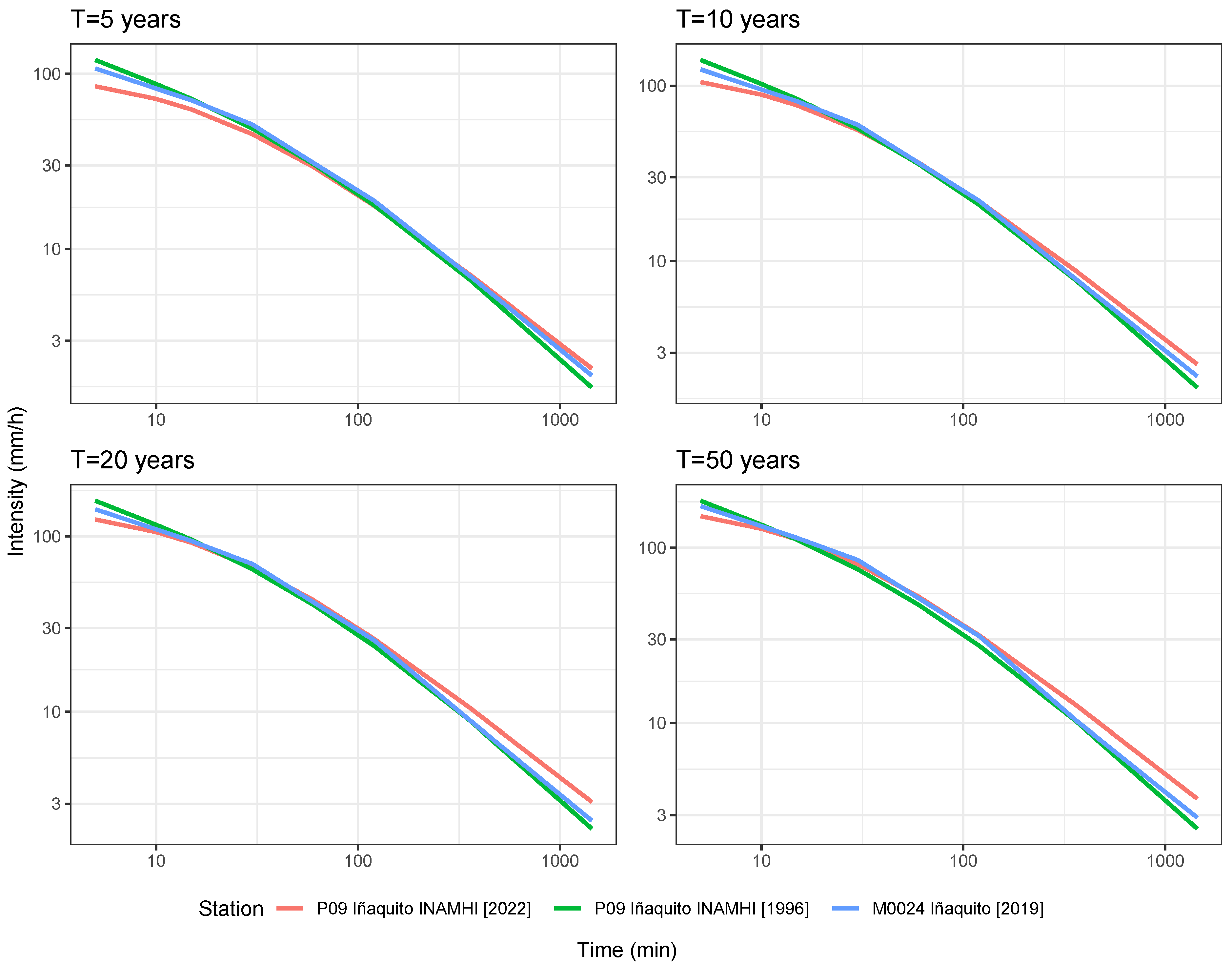
6.1. IDF Curves Comparison
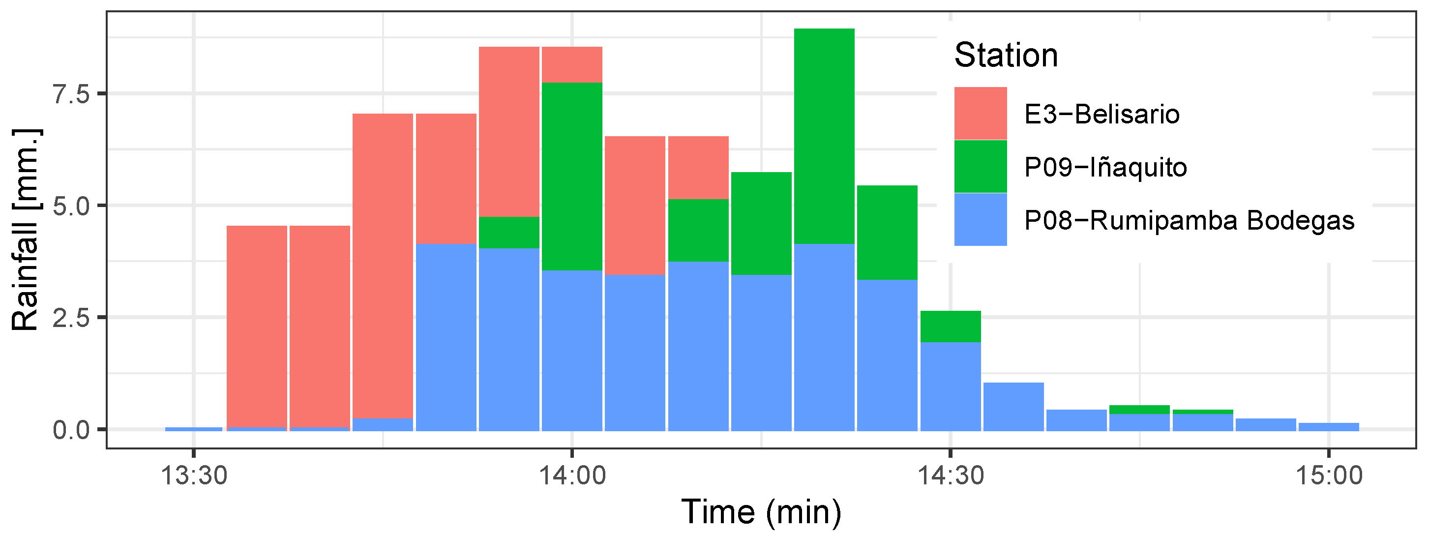
6.2. Grade Separation (Underpass) Flood in the North of Quito
6.3. La Gasca Lanslide
7. Conclusions
Author Contributions
Funding
Institutional Review Board Statement
Data Availability Statement
Acknowledgments
Conflicts of Interest
Abbreviations
| Term | Description |
| EPMAPS | Empresa Pública Metropolitana de Agua Potable y Saneamiento del Distrito |
| Metropolitano de Quito | |
| SADMQ | Secretaría de Ambiente del Distrito Metropolitano de Quito |
| ECAP | Estación Científica Agua y Páramo |
| FONAG | Fondo para la Protección del Agua |
| AIC | Akaike Information Criterion |
| BIC | Bayesian Information Criterion |
| IDF | Intensity-Duration-Frequency |
| IDW | Inverse Distance Weighting |
| MAE | Mean Absolute Error |
| MAPE | Mean Absolute Percentage Error |
| RMSE | Root Mean Square Error |
| NSE | Nash-Sutcliffe model efficiency coefficient |
| PBIAS | Percent Bias |
Appendix A
Appendix A.1

| Station Name | Code | Institution | IDF Equation (mm/min) |
|---|---|---|---|
| Rumihurco | C02 | EPMAPS | |
| Rumipamba | C04 | EPMAPS | |
| Bellavista | C05 | EPMAPS | |
| Rumihurco Machángara | P03 | EPMAPS | |
| Rumipamba Bodegas | P08 | EPMAPS | |
| Iñaquito INAMHI | P09 | EPMAPS | |
| Antenas | P11 | EPMAPS | |
| Toctiuco | P12 | EPMAPS | |
| San Francisco | P27 | EPMAPS | |
| Cruz Loma | P28 | EPMAPS | |
| Belisario | E3 | SADMQ | |
| Jipijapa | E4 | SADMQ |
Appendix A.2

References
- WHO. Atlas of Health and Climate; E-Book:WHO Press, World Health Organization (WHO): Geneva, Switzerland, 2012; Available online: https://www.who.int/publications/i/item/9789241564526 (accessed on 16 September 2022).
- Pelosi, A.; Furcolo, P.; Rossi, F.; Villani, P. The characterization of extraordinary extreme events (EEEs) for the assessment of design rainfall depths with high return periods. Hydrol. Process. 2020, 34, 2543–2559. [Google Scholar] [CrossRef]
- Mohymont, B.; Demarée, G.R.; Faka, D.N. Establishment of IDF-curves for precipitation in the tropical area of Central Africa—Comparison of techniques and results. Nat. Hazards Earth Syst. Sci. 2004, 4, 375–387. [Google Scholar] [CrossRef]
- Al-Amri, N.S.; Subyani, A.M. Generation of Rainfall Intensity Duration Frequency (IDF) Curves for Ungauged Sites in Arid Region. Earth Syst. Environ. 2017, 1, 8. [Google Scholar] [CrossRef]
- Wagesho, N.; Claire, M. Analysis of rainfall intensity-duration-frequency relationship for Rwanda. J. Water Resour. Prot. 2016, 8, 706. [Google Scholar] [CrossRef]
- Minh, H.V.T.; Lavane, K.; Lanh, L.T.; Thinh, L.V.; Cong, N.P.; Ty, T.V.; Downes, N.K.; Kumar, P. Developing Intensity-Duration-Frequency (IDF) Curves Based on Rainfall Cumulative Distribution Frequency (CDF) for Can Tho City, Vietnam. Earth 2022, 3, 866–880. [Google Scholar] [CrossRef]
- Kareem, D.A.; M Amen, A.R.; Mustafa, A.; Yüce, M.I.; Szydłowski, M. Comparative Analysis of Developed Rainfall Intensity–Duration–Frequency Curves for Erbil with Other Iraqi Urban Areas. Water 2022, 14, 419. [Google Scholar] [CrossRef]
- Shrestha, A.; Babel, M.S.; Weesakul, S.; Vojinovic, Z. Developing Intensity–Duration–Frequency (IDF) curves under climate change uncertainty: The case of Bangkok, Thailand. Water 2017, 9, 145. [Google Scholar] [CrossRef]
- Huff, F.A. Time distribution of rainfall in heavy storms. Water Resour. Res. 1967, 3, 1007–1019. [Google Scholar] [CrossRef]
- Balbastre-Soldevila, R.; García-Bartual, R.; Andrés-Doménech, I. A Comparison of Design Storms for Urban Drainage System Applications. Water 2019, 11, 757. [Google Scholar] [CrossRef]
- Sun, Y.; Wendi, D.; Kim, D.E.; Liong, S.Y. Deriving intensity–duration–frequency (IDF) curves using downscaled in situ rainfall assimilated with remote sensing data. Geosci. Lett. 2019, 6, 17. [Google Scholar] [CrossRef]
- Kawara, A.Q.; Elsebaie, I.H. Development of Rainfall Intensity, Duration and Frequency Relationship on a Daily and Sub-Daily Basis (Case Study: Yalamlam Area, Saudi Arabia). Water 2022, 14, 897. [Google Scholar] [CrossRef]
- Ghebreyesus, D.T.; Sharif, H.O. Development and Assessment of High-Resolution Radar-Based Precipitation Intensity-Duration-Curve (IDF) Curves for the State of Texas. Remote Sens. 2021, 13, 2890. [Google Scholar] [CrossRef]
- Ayabaca, E.; Cruz, F.; Gutiérrez, C. Curvas Intensidad-Duración-Frecuencia de Principales Estaciones Pluviográficas de Quito; Technical Report; EMAAP-Quito: Quito, Ecuador, 1996. [Google Scholar]
- INAMHI. Determinación de Ecuaciones para el Cálculo de Intensidades Máximas de Precipitación; Technical Report; Instituto Nacional Meteorológico e Hidrológico: Quito, Ecuador, 2019. [Google Scholar]
- Zevallos, J.; Gutiérrez, R.; Lavado, W. Generación de Curvas Intensidad-Duración-Frecuencia en Perú; Pontificia Universidad Católica del Perú Tesis Lima: Perú, Ecuador, 2019. [Google Scholar]
- Jove, F.; Hernández, R.; Caballero, A. IDF Curves and Maximum Rainfall in 24 hours in the Subregions of La Mojana and San Jorge in Northern Colombia. Int. J. Eng. Res. Technol. 2020, 13, 2884–2894. [Google Scholar] [CrossRef]
- Bertoni, J.C.; Martínez, F.M.G.; Brarda, J.P.; Tibaldo, O.; Rudolf, C.; Verga, L. Actualización de Relaciones Iintensidad-Duración-Frecuencia (IDF) de la Ciudad de Rafaela (Provincia de Santa Fe, Argentina). II Taller Sobre Reg. Precip. Máximas 2009, 2, 8. [Google Scholar]
- Casas, M.C.; Codina, B.; Redaño, A.; Lorente, J. A methodology to classify extreme rainfall events in the western Mediterranean area. Theor. Appl. Climatol. 2004, 77, 139–150. [Google Scholar] [CrossRef]
- Casas Castillo, M.C. Análisis Espacial y Temporal de las Lluvias Extremas en Catalunya. Modelización y Clasificación Objetiva. Ph.D. Thesis, Departament d’Astronomia i Meteorologia, Universidad de Barcelona, Barcelona, Spain, 2005. [Google Scholar]
- Navarro Bosque, J. Organització Espacial i Temporal de la Pluja a L’àrea Metropolitana de Barcelona. Ph.D. Thesis, Universitat Politècnica de Catalunya, Barcelona, Spain, 2022. [Google Scholar]
- EPMAPS. Empresa Pública Metropolitana de Agua Potable Y Saneamiento. 2022. Available online: https://www.aguaquito.gob.ec/ (accessed on 16 September 2022).
- SADMQ. Secretaría de Ambiente del Distrito Metropolitano de Quito. 2022. Available online: www.quitoambiente.gob.ec (accessed on 16 September 2022).
- Garreaud, R.D. The Andes climate and weather. Adv. Geosci. 2009, 22, 3–11. [Google Scholar] [CrossRef]
- Marocco, R.; Winter, T. Capítulo 2-Bosquejo de la Evolución Geodinámica del Ecuador; Centro Ecuatoriano de Investigación Geográfica: Quito, Ecuador, 1997. [Google Scholar]
- Boschman, L.M. Andean mountain building since the Late Cretaceous: A paleoelevation reconstruction. Earth-Sci. Rev. 2021, 220, 103640. [Google Scholar] [CrossRef]
- Perrin, J.L.; Sierra, A.; Fourcade, B.; Poulenard, J.; Risser, V.; Janeau, J.L.; Gueguen, P.; Hubert, S. Quito Face a un Risque D’origine Naturelle la lave Torrentielle du 31 Mars 1997 dans le Quartier de la Comuna. Programme SISHILAD, EMAAP-Q, INAMHI, ORSTOM. 1997. Available online: https://www.researchgate.net/publication/32969940_Quito_face_a_un_risque_d%27origine_naturelle_la_lave_torrentielle_du_31_mars_1997_dans_le_quartier_de_La_Comuna (accessed on 16 September 2022).
- Quito-Informa. Epmaps Cuenta con la Red Hidrometeorológica Más Completa del país. 2022. Available online: http://www.quitoinforma.gob.ec/2022/05/19/epmaps-cuenta-con-la-red-hidrometeorologica-mas-completa-del-pais/ (accessed on 16 September 2022).
- SADMQ. Instituto Nacional de Meteorología e Hidrología. 2022. Available online: https://www.inamhi.gob.ec/ (accessed on 16 September 2022).
- Lana, X.; Rodríguez-Solà, R.; Martínez, M.; Casas-Castillo, M.; Serra, C.; Burgueño, A. Characterization of standardized heavy rainfall profiles for Barcelona city: Clustering, rain amounts and intensity peaks. Theor. Appl. Climatol. 2020, 142, 255–268. [Google Scholar] [CrossRef]
- Akaike, H. A new look at the statistical model identification. IEEE Trans. Autom. Control 1974, 19, 716–723. [Google Scholar] [CrossRef]
- Schwarz, G. Estimating the dimension of a model. Ann. Stat. 1978, 6, 461–464. [Google Scholar] [CrossRef]
- Moss, J. univariateML: An R package for maximum likelihood estimation of univariate densities. J. Open Source Softw. 2019, 4, 1863. [Google Scholar] [CrossRef]
- Borchers, H.W.; Borchers, M.H.W. Package “Pracma”. 2022. Available online: https://mirror.las.iastate.edu/CRAN/web/packages/pracma/pracma.pdf (accessed on 16 September 2022).
- Sherman, C.W. Frequency and intensity of excessive rainfalls at Boston, Massachusetts. Trans. Am. Soc. Civ. Eng. 1931, 95, 951–960. [Google Scholar] [CrossRef]
- Team, R.C.; Team, M.R.C.; Suggests, M.; Matrix, S. Package “Stats”. In The R Stats Package; R Foundation for Statistical Computing: Vienna, Austria, 2018. [Google Scholar]
- Zambrano-Bigiarini, M. hydroGOF: Goodness-of-Fit Functions for Comparison of Simulated and Observed Hydrological Time Series. R Package Version 0.4-0; Zenodo, 2020. [Google Scholar] [CrossRef]
- Moriasi, D.N.; Gitau, M.W.; Pai, N.; Daggupati, P. Hydrologic and water quality models: Performance measures and evaluation criteria. Trans. ASABE 2015, 58, 1763–1785. [Google Scholar]
- De Myttenaere, A.; Golden, B.; Le Grand, B.; Rossi, F. Mean absolute percentage error for regression models. Neurocomputing 2016, 192, 38–48. [Google Scholar] [CrossRef]
- Erazo, B.; Bourrel, L.; Frappart, F.; Chimborazo, O.; Labat, D.; Dominguez-Granda, L.; Matamoros, D.; Mejia, R. Validation of satellite estimates (Tropical Rainfall Measuring Mission, TRMM) for rainfall variability over the Pacific slope and Coast of Ecuador. Water 2018, 10, 213. [Google Scholar] [CrossRef]
- Ruelland, D. Should altitudinal gradients of temperature and precipitation inputs be inferred from key parameters in snow-hydrological models? Hydrol. Earth Syst. Sci. 2020, 24, 2609–2632. [Google Scholar] [CrossRef]
- Erazo, B. Representing Past and Future Hydro-Climatic Variability over Multi-Decadal Periods in Poorly-Gauged Regions: The Case of Ecuador. Ph.D. Thesis, Université Paul Sabatier-Toulouse III, Toulouse, France, 2020. [Google Scholar]
- González-Zeas, D.; Erazo, B.; Lloret, P.; De Bièvre, B.; Steinschneider, S.; Dangles, O. Linking global climate change to local water availability: Limitations and prospects for a tropical mountain watershed. Sci. Total Environ. 2019, 650, 2577–2586. [Google Scholar] [CrossRef]
- Brath, A.; Castellarin, A.; Montanari, A. Assessing the reliability of regional depth-duration-frequency equations for gaged and ungaged sites. Water Resour. Res. 2003, 39, 1367. [Google Scholar] [CrossRef]
- Hodson, T.O. Root mean square error (RMSE) or mean absolute error (MAE): When to use them or not. Geosci. Model Dev. Discuss. 2022, 15, 5481–5487. [Google Scholar] [CrossRef]
- Un Aguacero Anega las Calles de Quito. 2017. Available online: https://www.elcomercio.com/actualidad/quito/quito-lluvias-inundacion-emergencias-coe.html (accessed on 16 September 2022).
- Bader, M.; Forbes, G.; Grant, J.; Lilley, R.; Waters, A. Images in Weather Forecasting. A Practical Guide for Interpreting Satellite and Radar Imagery; Cambridge University Press: Cambridge, UK, 1995. [Google Scholar]
- Ecuador: Deadly Landslide after Heaviest Rainfall in Years. 2022. Available online: www.bbc.com/news/world-latin-america-60211539 (accessed on 16 September 2022).
- Regen Verursacht Katastrophe in Quito. 2022. Available online: https://p.dw.com/p/46OY9 (accessed on 16 September 2022).
- Léa Hurel, Ecuador: Comienza en Quito la Remoción de Escombros tras el Aluvión que dejó Decenas de Muertos. 2022. Available online: https://www.france24.com/es/am%C3%A9rica-latina/20220204-ecuador-aluvion-quito-lluvias-remocion (accessed on 16 September 2022).


| Samples | P09 | P11 | P12 | P03 | C02 | C05 | P27 | P28 | P08 | C04 | E3 | E4 |
|---|---|---|---|---|---|---|---|---|---|---|---|---|
| Count | 1,990,857 | 1,935,434 | 1,940,010 | 1,957,995 | 1,840,723 | 1,993,251 | 1,726,967 | 1,844,597 | 2,035,963 | 1,839,566 | 1,296,022 | 1,217,532 |
| Mean | 0.009 | 0.012 | 0.01 | 0.01 | 0.009 | 0.009 | 0.013 | 0.014 | 0.012 | 0.012 | 0.01 | 0.005 |
| STD | 0.093 | 0.101 | 0.104 | 0.095 | 0.087 | 0.094 | 0.114 | 0.103 | 0.113 | 0.109 | 0.109 | 0.06 |
| 99th PCTL | 2.3 | 2.2 | 2.5 | 2.3 | 2 | 2.4 | 2.64 | 2 | 2.7 | 2.4 | 2.55 | 1.7 |
| Max | 10.3 | 7.6 | 8.6 | 10.1 | 7.1 | 9.7 | 10.2 | 8.64 | 9.12 | 9.1 | 10 | 8.2 |
| Duration [min.] | E [Number of Events] | Max [mm.] | Mean [mm.] | Standard Deviation |
|---|---|---|---|---|
| 5 | 20,470 | 10.3 | 0.2623 | 0.5336 |
| 10 | 14,106 | 20.2 | 0.4791 | 1.0667 |
| 15 | 11,536 | 27.3 | 0.6848 | 1.5079 |
| 20 | 10,073 | 31.6 | 0.8727 | 1.8778 |
| 25 | 9138 | 34.1 | 1.0394 | 2.1902 |
| 30 | 8443 | 35.6 | 1.1877 | 2.4603 |
| 35 | 7903 | 40.2 | 1.3212 | 2.6935 |
| 40 | 7498 | 42.8 | 1.4448 | 2.8962 |
| 45 | 7163 | 43.2 | 1.5534 | 3.0658 |
| 50 | 6907 | 43.4 | 1.6534 | 3.2138 |
| 55 | 6684 | 43.9 | 1.7424 | 3.3466 |
| 60 | 6425 | 44.3 | 1.8457 | 3.4829 |
| 65 | 6251 | 44.4 | 1.9286 | 3.5985 |
| 70 | 6095 | 44.5 | 2.0015 | 3.7012 |
| 75 | 5952 | 45.8 | 2.0713 | 3.7954 |
| 120 | 5025 | 60.8 | 2.6227 | 4.5085 |
| 240 | 3888 | 66.3 | 3.6254 | 5.6186 |
| 360 | 3289 | 66.4 | 4.3987 | 6.3900 |
| 540 | 2640 | 67.8 | 5.2310 | 7.2511 |
| 720 | 2164 | 73.9 | 6.0195 | 8.0285 |
| 840 | 1958 | 74 | 6.4143 | 8.4635 |
| 960 | 1778 | 74 | 6.7807 | 8.8716 |
| 1080 | 1624 | 74 | 7.1826 | 9.3408 |
| 1200 | 1511 | 74 | 7.5331 | 9.7840 |
| 1320 | 1365 | 74.1 | 8.1012 | 10.4412 |
| 1440 | 1230 | 74.3 | 8.8395 | 11.2411 |
| Duration (min) | k | |
|---|---|---|
| 5 | 0.2417 | 0.9213 |
| 10 | 0.2017 | 0.4211 |
| 15 | 0.2062 | 0.3012 |
| 20 | 0.2160 | 0.2475 |
| 25 | 0.2252 | 0.2167 |
| 30 | 0.2331 | 0.1962 |
| 35 | 0.2406 | 0.1821 |
| 40 | 0.2489 | 0.1723 |
| 45 | 0.2567 | 0.1653 |
| 50 | 0.2647 | 0.1601 |
| 55 | 0.2711 | 0.1556 |
| 60 | 0.2808 | 0.1521 |
| 65 | 0.2872 | 0.1489 |
| 70 | 0.2924 | 0.1461 |
| 75 | 0.2978 | 0.1438 |
| 120 | 0.3384 | 0.1290 |
| 240 | 0.4163 | 0.1148 |
| 360 | 0.4739 | 0.1077 |
| 540 | 0.5204 | 0.0995 |
| 720 | 0.5621 | 0.0934 |
| 840 | 0.5744 | 0.0895 |
| 960 | 0.5842 | 0.0862 |
| 1080 | 0.5913 | 0.0823 |
| 1200 | 0.5928 | 0.0787 |
| 1320 | 0.6020 | 0.0743 |
| 1440 | 0.6184 | 0.0700 |
| Station Code | MAE | RMSE | NSE | MAPE | R2 |
|---|---|---|---|---|---|
| C02 | 2.8161 | 4.0359 | 0.9465 | 0.0336 | 0.9634 |
| C04 | 2.1601 | 3.2093 | 0.9789 | 0.0580 | 0.9809 |
| C05 | 4.0822 | 4.8267 | 0.9019 | 0.0240 | 0.9231 |
| P03 | 3.7254 | 6.8351 | 0.8812 | 0.0325 | 0.9128 |
| P08 | 1.9533 | 3.3155 | 0.9700 | 0.0238 | 0.9757 |
| P09 | 2.9906 | 3.6563 | 0.9620 | 0.0502 | 0.9852 |
| P11 | 2.2183 | 3.2757 | 0.9837 | 0.0548 | 0.9909 |
| P12 | 6.9881 | 9.1153 | 0.8908 | 0.0724 | 0.9446 |
| P27 | 2.6436 | 3.3288 | 0.9749 | 0.0279 | 0.9776 |
| P28 | 3.6275 | 4.4120 | 0.9524 | 0.1384 | 0.9692 |
| E3 | 3.8009 | 4.6277 | 0.9130 | 0.0889 | 0.9182 |
| E4 | 3.3063 | 4.1126 | 0.8370 | 0.1060 | 0.9410 |
| Average | 3.3594 | 4.5626 | 0.9327 | 0.0592 | 0.9569 |
| Station | MAE | RMSE | NSE | MAPE | R2 |
|---|---|---|---|---|---|
| P09-2022 1 | 2.9906 | 3.6563 | 0.9620 | 0.0502 | 0.9852 |
| P09-1996 2 | 9.2461 | 14.1971 | 0.9049 | 0.1679 | 0.9343 |
| M0024-2019 3 | 7.1453 | 9.7829 | 0.9548 | 0.1310 | 0.9600 |
Publisher’s Note: MDPI stays neutral with regard to jurisdictional claims in published maps and institutional affiliations. |
© 2022 by the authors. Licensee MDPI, Basel, Switzerland. This article is an open access article distributed under the terms and conditions of the Creative Commons Attribution (CC BY) license (https://creativecommons.org/licenses/by/4.0/).
Share and Cite
Escobar-González, D.; Singaña-Chasi, M.S.; González-Vergara, J.; Erazo, B.; Zambrano, M.; Acosta, D.; Villacís, M.; Guallpa, M.; Lahuatte, B.; Peluffo-Ordóñez, D. Intensity-Duration-Frequency Curve for Extreme Rainfall Event Characterization, in the High Tropical Andes. Water 2022, 14, 2998. https://doi.org/10.3390/w14192998
Escobar-González D, Singaña-Chasi MS, González-Vergara J, Erazo B, Zambrano M, Acosta D, Villacís M, Guallpa M, Lahuatte B, Peluffo-Ordóñez D. Intensity-Duration-Frequency Curve for Extreme Rainfall Event Characterization, in the High Tropical Andes. Water. 2022; 14(19):2998. https://doi.org/10.3390/w14192998
Chicago/Turabian StyleEscobar-González, Diego, Mélany S. Singaña-Chasi, Juan González-Vergara, Bolívar Erazo, Miguel Zambrano, Darwin Acosta, Marcos Villacís, Mario Guallpa, Braulio Lahuatte, and Diego H. Peluffo-Ordóñez. 2022. "Intensity-Duration-Frequency Curve for Extreme Rainfall Event Characterization, in the High Tropical Andes" Water 14, no. 19: 2998. https://doi.org/10.3390/w14192998
APA StyleEscobar-González, D., Singaña-Chasi, M. S., González-Vergara, J., Erazo, B., Zambrano, M., Acosta, D., Villacís, M., Guallpa, M., Lahuatte, B., & Peluffo-Ordóñez, D. (2022). Intensity-Duration-Frequency Curve for Extreme Rainfall Event Characterization, in the High Tropical Andes. Water, 14(19), 2998. https://doi.org/10.3390/w14192998