

Three-Dimensional Engineering Geological Model and Its Applications for a Landslide Site: Combination of Grid- and Vector-Based Methods

 ,
,  , , ,
, , ,
Abstract
1. Introduction
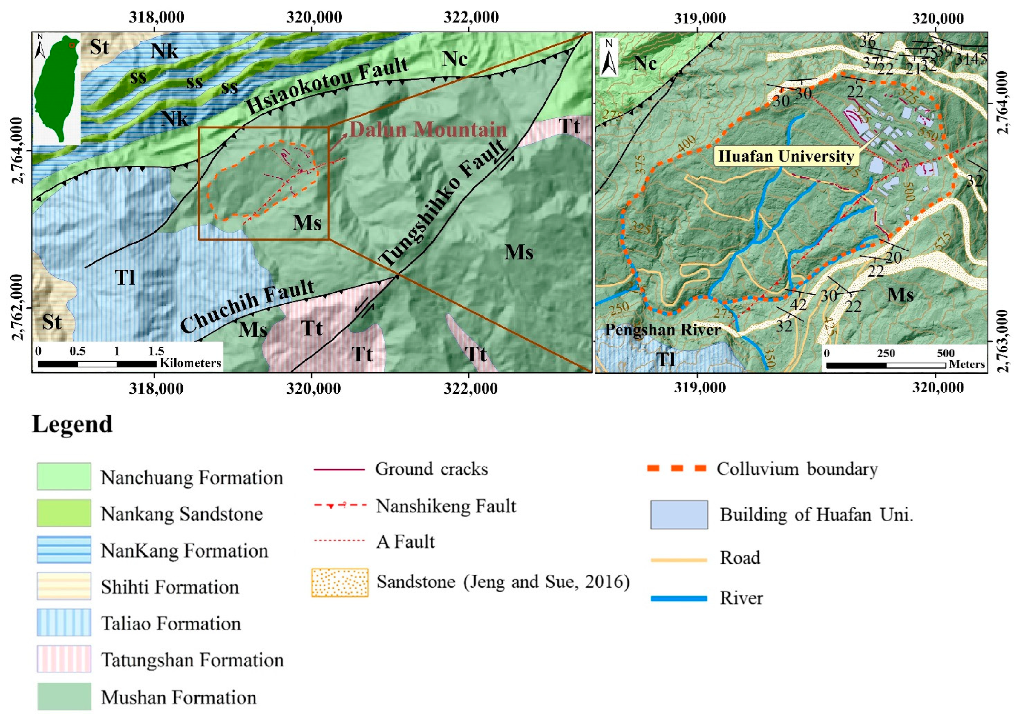
2. Study Area
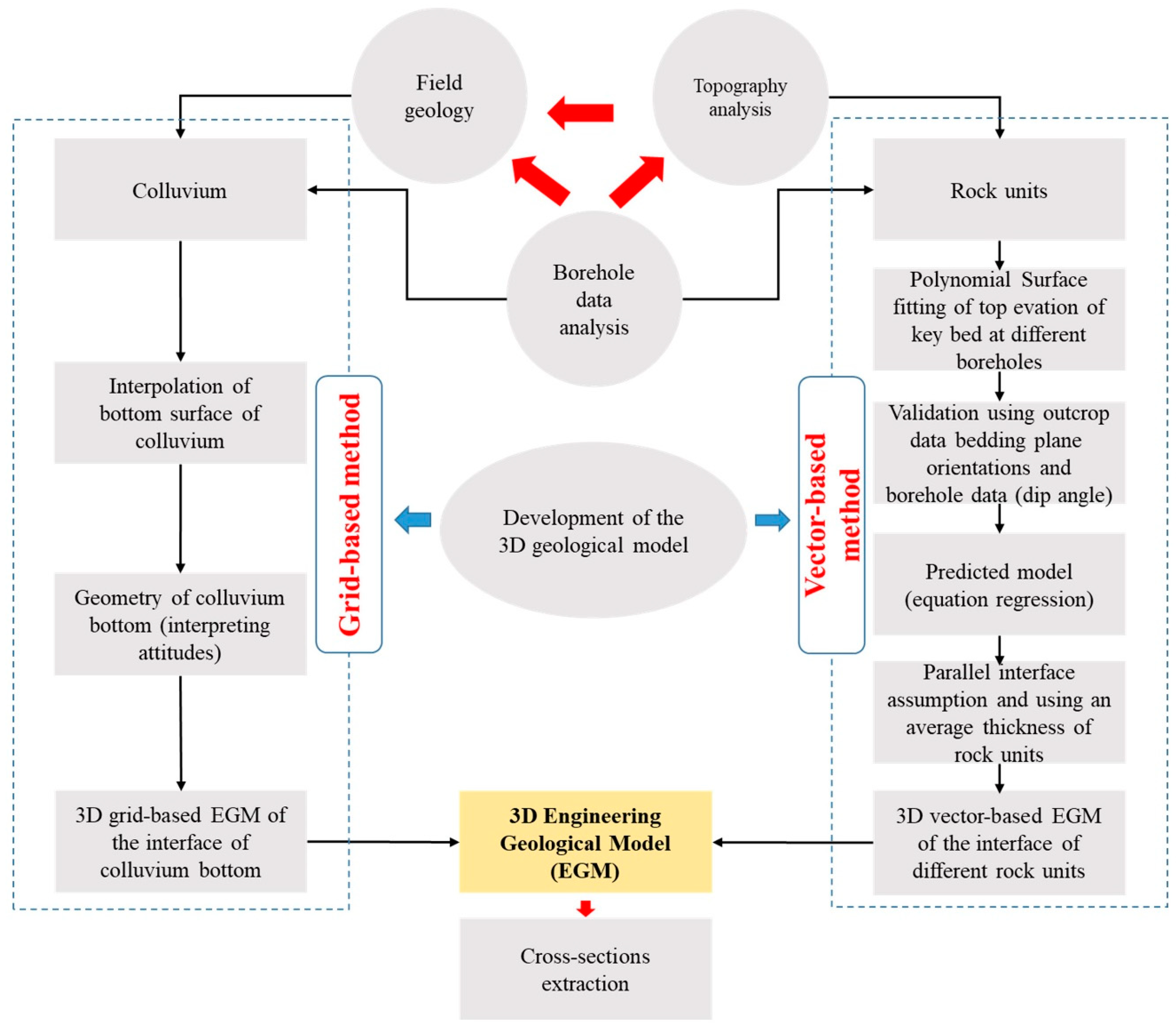
3. Methodology to Develop a 3D EGM
3.1. Topography Analysis
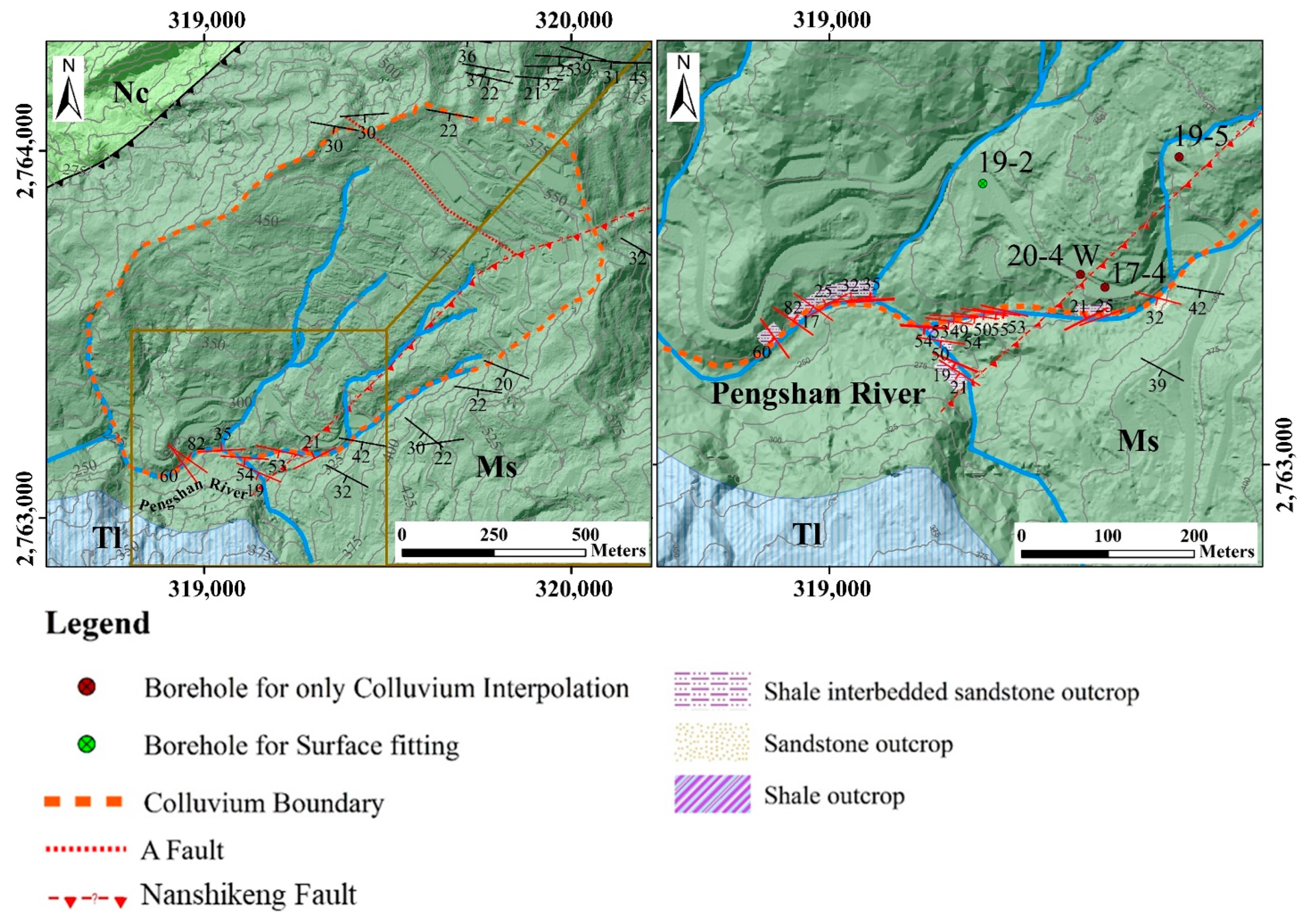
3.2. Field Investigation
3.3. Borehole Data Analysis
- (1)
- Borehole data quality check. To begin, we thoroughly checked the reported locations and elevations of the boreholes, in order to ensure the correctness of the basic information. If the X and Y input values were inaccurate, the elevation of each borehole will be changed significantly, such that the elevation of the rock unit boundary will also be misjudged. The TWD97 TM2 (i.e., Taiwan Datum 1997, 2-degree Transverse Mercator) coordinate system was employed in this work, in order to ensure data coherence. As a result, this step is critical for further analysis. We used the LiDAR DEM to obtain the elevations (i.e., Z values) of the boreholes at given horizontal coordinates (i.e., X for E–W direction and Y for N–S direction), and compared them with the documented elevations of boreholes. In addition, the quality of the rock core must not have been significantly impacted by weathering (i.e., preserved in fresh bedrock) or shearing or fracturing by tectonic processes. We preferred boreholes with an adequate depth, which permit comparisons between a sequence of units in different boreholes. Only the boreholes that passed this checking step were used for subsequent 3D EGM development. In this way, we ensured that only reliable borehole data were considered prior to the following steps.
- (2)
- Rock unit classification. The fundamental interpretation consisted of lithology identification and rock unit boundary determination. Sandstone (SS) and thin alternating layers of sandstone and shale (SS and SH, respectively) constitute the main lithology in the study area. The sedimentary features of rock units, such as whitish sandstone, particularly form thick or massive layers. The grayish-black shale and thin interbeds of sandstone and shale are also well-developed, often alternating with thick sandstones [28]. The sedimentary sequences were considered when we analyzed the rock cores; in particular, we considered a sequence of continuous rock units throughout the borehole, as opposed to focusing on a single rock unit (i.e., homogeneous in a sequence of rock units). Lithostratigraphic bodies were distinguished by distinct lithological minor structures, such as lamina and flaser structures, as a criterion for determining the sedimentary sequence. The proportion of sandstones and shales was used to classify the alternated layers of sandstone and shale into different rock units. The descriptive reference proportions are:
- (I)
- Interlayer 1:1 ≤ Mj:Mn ≤2:1,
- (II)
- Interbedded 2:1 ≤ Mj:Mn ≤ 4:1,
- (III)
- Occasionally 4:1 ≤ Mj:Mn ≤ 8:1,
- (IV)
- Main lithology 8:1 ≤ Mj:Mn,
where Mj denotes major lithology and Mn denotes minor lithology.
- (3)
- Comparison between rock units from different boreholes. In the advanced step, we conducted a comparison of the lithology from the 26 complete boreholes among the 50 boreholes in the study area, in order to prepare the necessary material for the building of the geological model. To make the comparisons accessible and reliable, we started with the boreholes that were close to each other. We grouped the boreholes together and compared the lithology of the strata. We assumed that the features of the strata lithology of these boreholes should be the same; however, the boreholes were distributed sporadically and also outside the campus on the downward slope. Both petrographic properties and the distribution of boreholes had changed slightly. When the rock cores were compared to each other, this aspect also had been carefully considered. There are comparison criteria that may be depended upon to ensure reliability. In this context, sedimentary characteristics, including the texture and internal structures created by bioturbation and bio-erosion, are essential for classifying rock units to build correlatively connected boreholes. Furthermore, every objective layer’s thickness must have minimal change; that is, the standard deviation of the thickness should be small. Furthermore, a structural dip was recognized in the borehole description and the rock core photos, handled in laminated or thinly bedded to bedded shale and sandstone sequences. Such a structural dip is best-identified from cross-bedded sections thought to have been horizontally stratified originally, which we call cross-bedding, accordingly. As a result, a side-by-side comparison of lithological borehole data was conducted.
- (4)
- Selection of key marker bed. The thick sandstone was selected as the key bed of the rock unit, as it was readily distinguishable. To obtain a reliable result, the thick sandstone must be identifiable over a large number of boreholes (i.e., be unique and widespread), ensuring that it exists at most locations in the study area through these boreholes. The sedimentary sequences are significant, as they help us to identify which sandstone is the proper one among the boreholes. This is based strictly on the distinguished lithology in the sedimentary sequences, as mentioned above (e.g., the laminated structure in the alternating sandstone and shale units). In addition, the key bed must fulfill the requirements for the comparison of rock units from different boreholes, as described in step (3) above.
3.4. Development of the 3D EGM
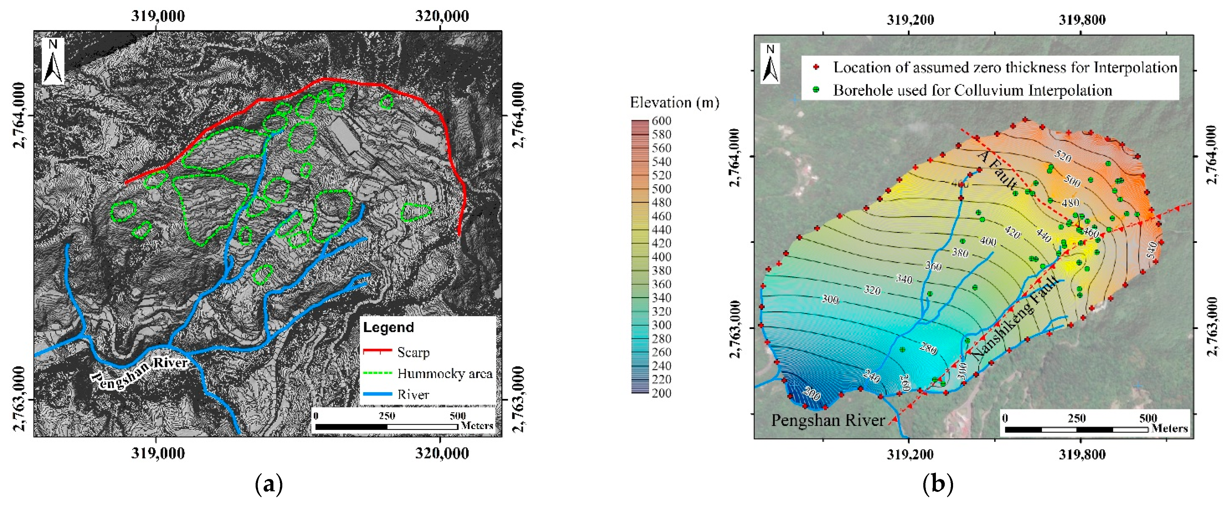
3.4.1. Interpolation of Colluvium Bottom Boundary (Depth of Bedrock Top Surface): Grid-Based Method
3.4.2. Determining the Polynomial Surfaces Representing the Rock Boundaries: Vector-Based Method
4. Results of 3D EGM Development
4.1. Boundary of Paleo Landslide Deposits
4.2. Grid-Based Interface between Colluvium and Bedrock
4.3. Geologically Uniform Zones
4.4. Development of Geological Model in Zones 1 and 2
4.4.1. Classification of Rock Units
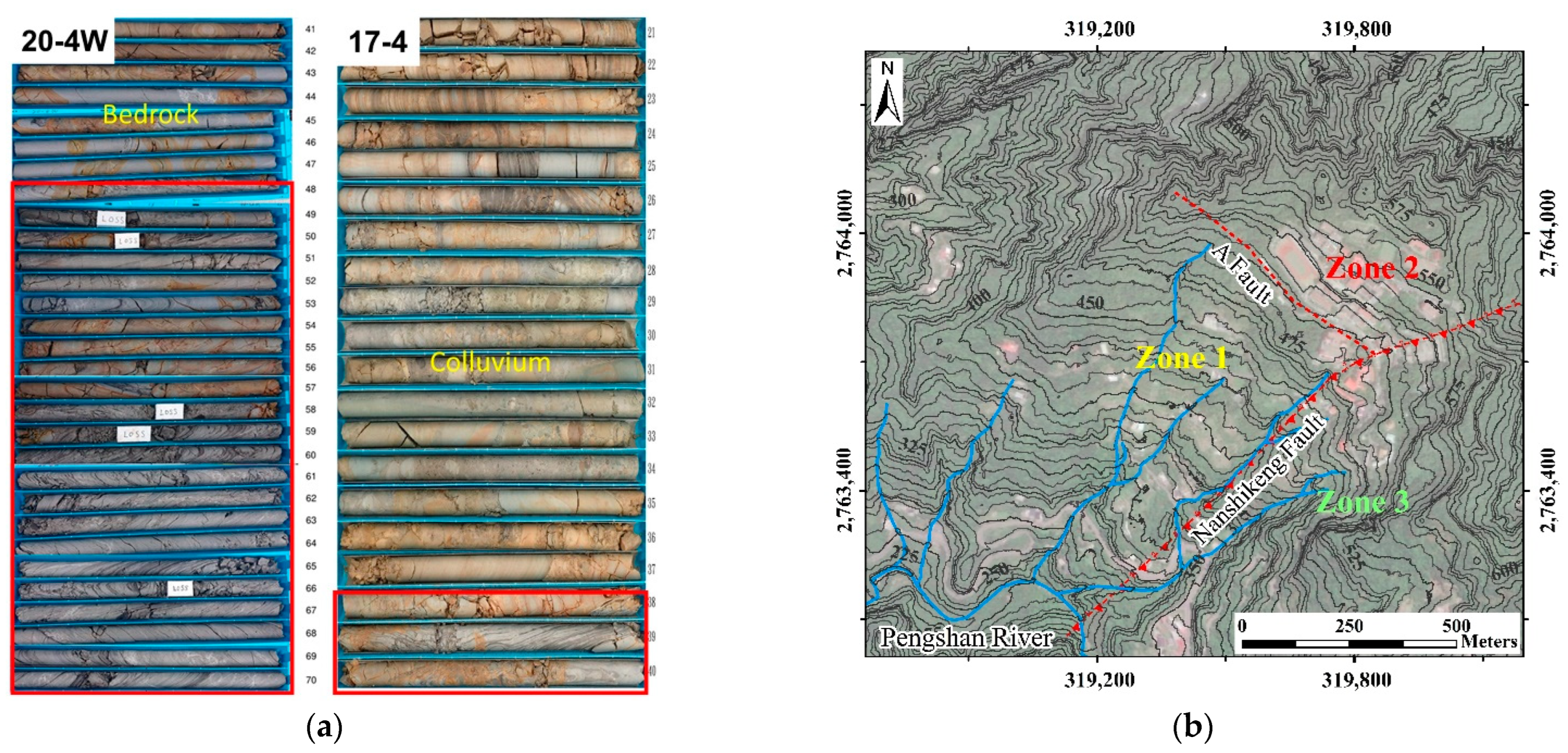
- Colluvium (Co). The cover material layer consists of loose and unconsolidated sediments characterized by weathered sandstone pieces and blocks with brownish color and gray matrices, fragments, debris, and soil. The fragments differ in size, shape, and crack density. In some boreholes, the fill material (dark yellowish, fine-grained) is fairly thick, which is due to the constructions, especially in the group of boreholes within the university campus. The thickness of the cover material varied, with the thickest section reaching approximately 40 m (borehole 17-4) towards the toe of the slope located to the southwest of the mountain. Based on the geological processing in the Mt. Dalun area, as well as topographical analysis, the colluvium may have originated from two sources: Loose material belonging to the ancient deep-seated landslides and so-called slope wash (i.e., debris slide).
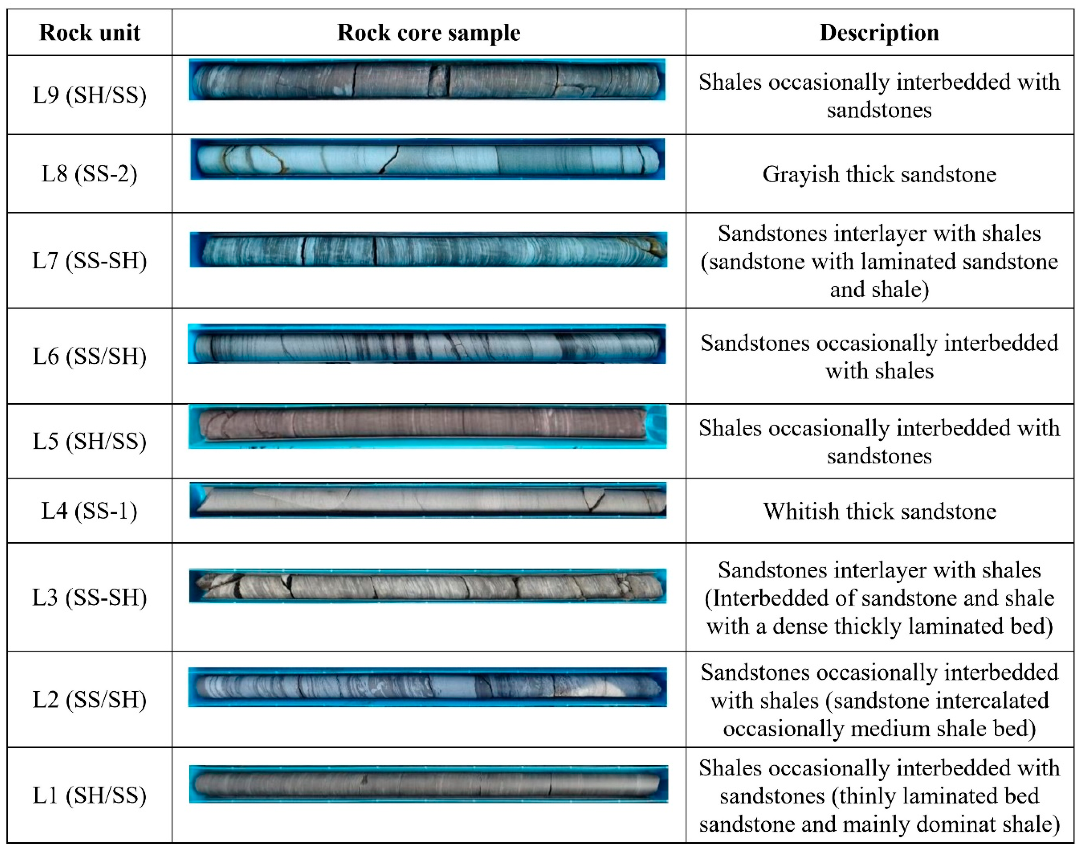
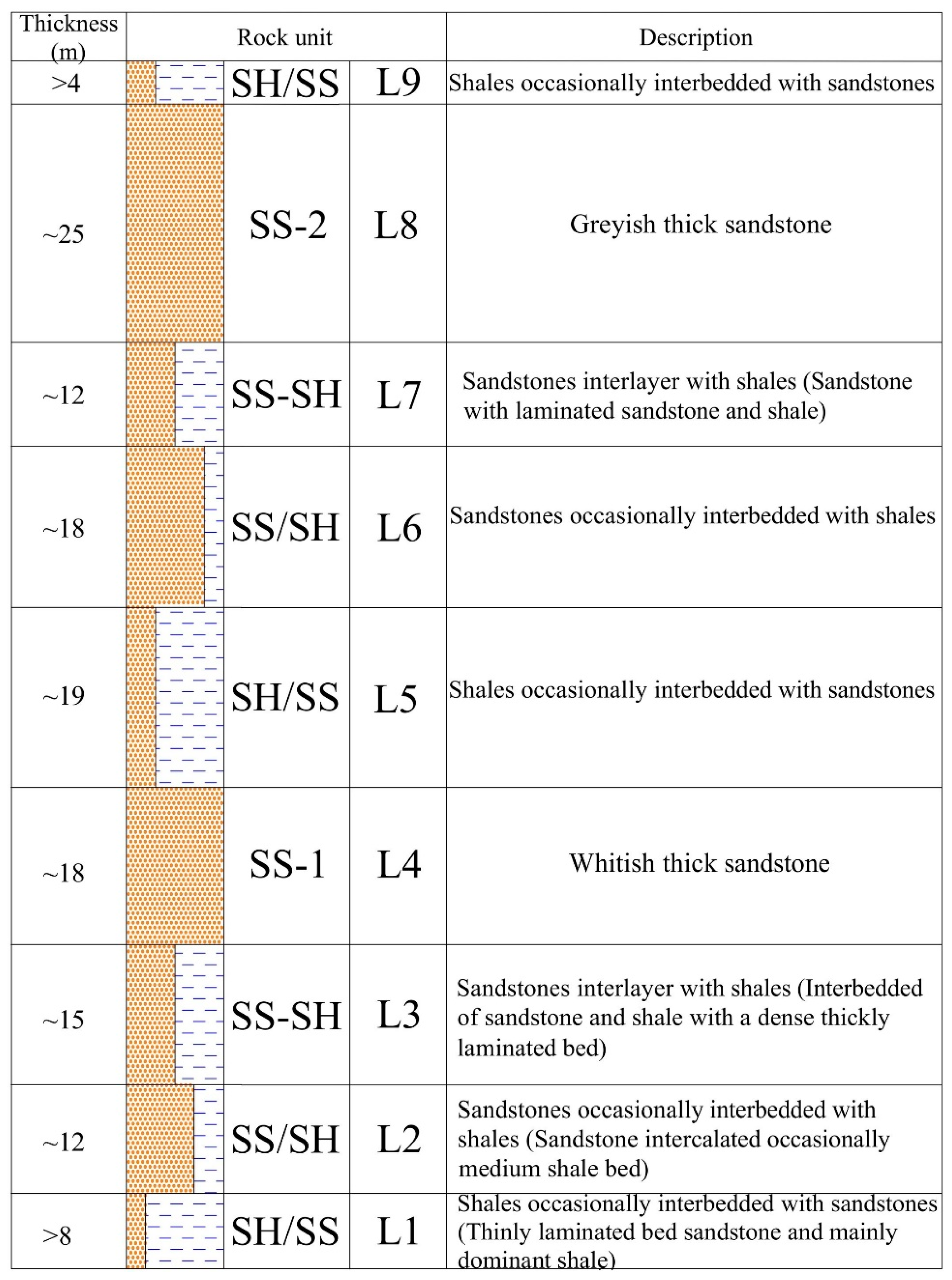
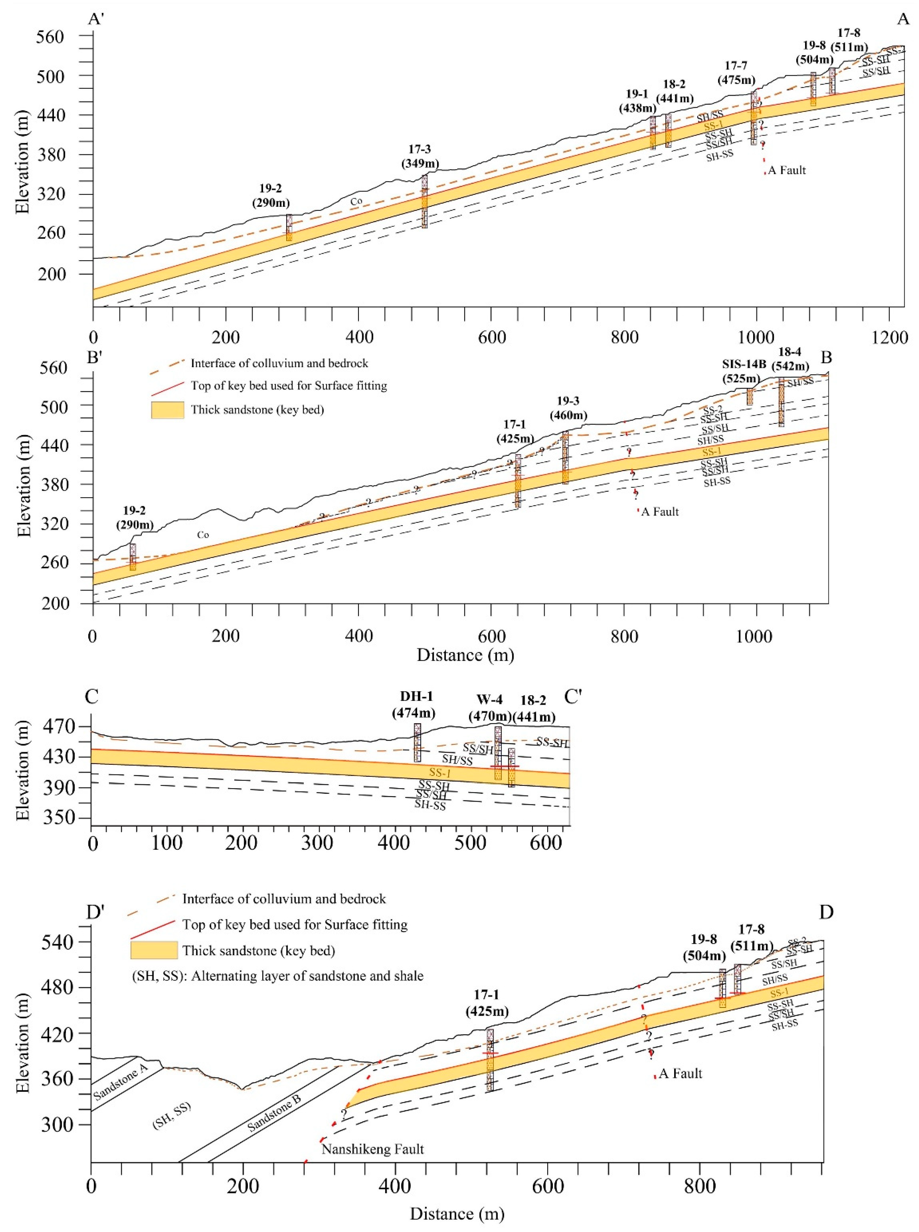
- Sandstone (SS). Two rock units were identified as sandstone: L4 (SS-1) and L8 (SS-2). The lithology in L4 was mostly composed of thick, medium-grained whitish sandstone intercalated with thin dark black shale layers scattered in a few places in the massive sandstone. A shear zone containing mud was found in some rock cores. The rock core contains a number of joints. As previously stated, L4 is a key bed identified in the sedimentary sequence, and the overlaying and underlying units are L5 and L3, respectively, characterized by laminated alternations of sandstone and shale. As for L8, grayish sandstone occasionally intercalated with laminated shale is the main lithology. L8 had a higher average thickness than L4, about 25 m and 16 m, respectively. Therefore, the L4 was comparatively identifiable from L8.
- Alternations of sandstone and shale (SS, SH). This type of rock unit included L1 (SH/SS), L2 (SS/SH), L3 (SS-SH), L5 (SH/SS), L6 (SS/SH), L7 (SS-SH), and L9 (SH/SS). The ratio of sandstone and shale proportion in the recovered rock core significantly varied among these rock units. Each rock unit is described, respectively, in the following:
- a.
- Rock unit SH/SS (Shales occasionally interbedded with sandstones). This rock is characterized by black to gray shale interbedded with fine sandstone, very thin-bedded sandstone and shale, and mainly dominant shale percentage. It contains sandstone and shale, with shale constituting up to 70–90% of the rock core.
- b.
- Rock unit SS-SH (Sandstones interlayered with shales). The lithology is composed of interbedded sandstone and black to gray shale, with the thickness ranging from thinly laminated to thickly laminated, and extremely thinly bedded. The sandstone content throughout the portion is approximately 50%, with beds containing parallel lamination and, occasionally, ripple cross-stratification.
- c.
- Rock unit SS/SH (Sandstones occasionally interbedded with shales). The lithology composed of gray to whitish sandstone is the dominant lithology, with black shale interspersed and occasionally locally interbedded sandstone and shale. The sandstone beds range from medium bedded to very thickly bedded, accounting for about 70–80% of the composition.
4.4.2. Upper Boundary of Key Bed
4.4.3. The Average Thickness of Each Rock Unit in Zones 1 and 2
4.5. Development of Geological Model in Zone 3
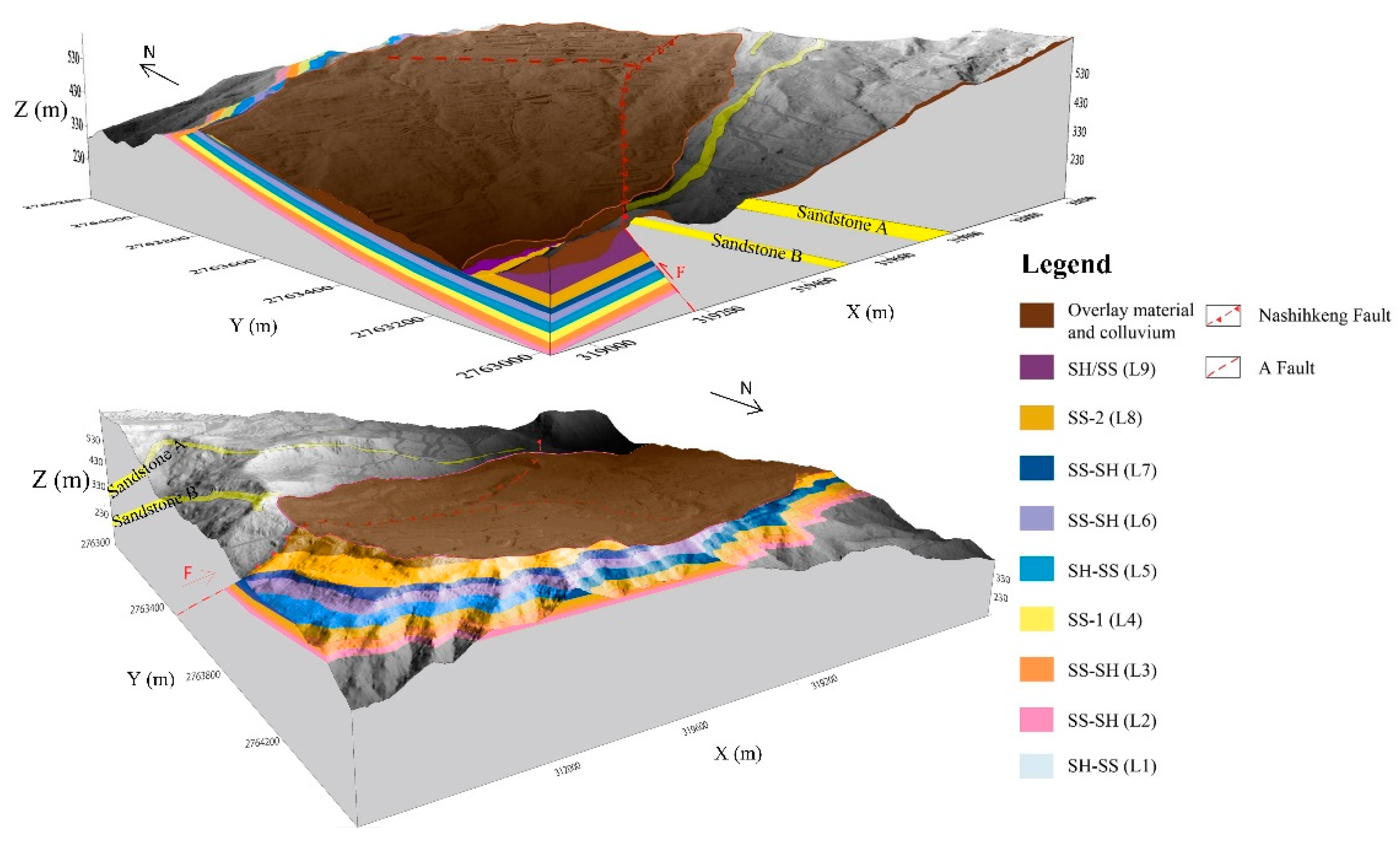
4.6. Three-Dimensional Engineering Geological Model and Geological Profiles
5. Applications of the 3D EGM
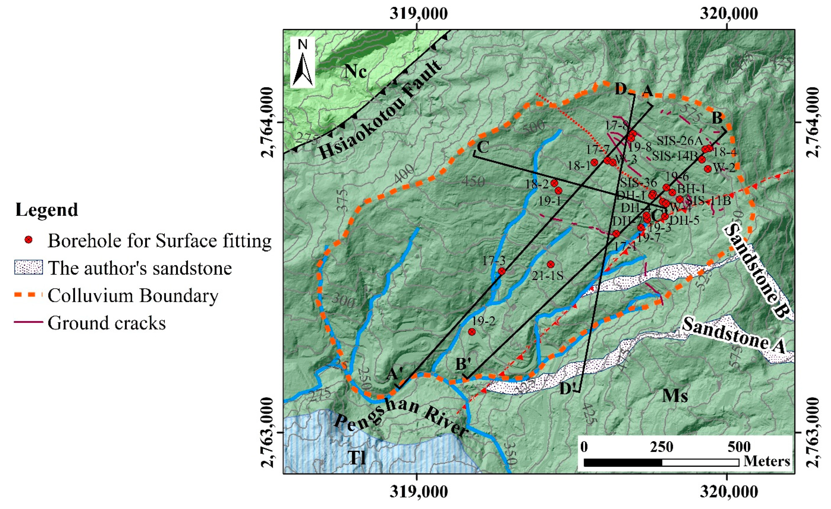
5.1. Surface and Sub-Surface Displacement Monitoring
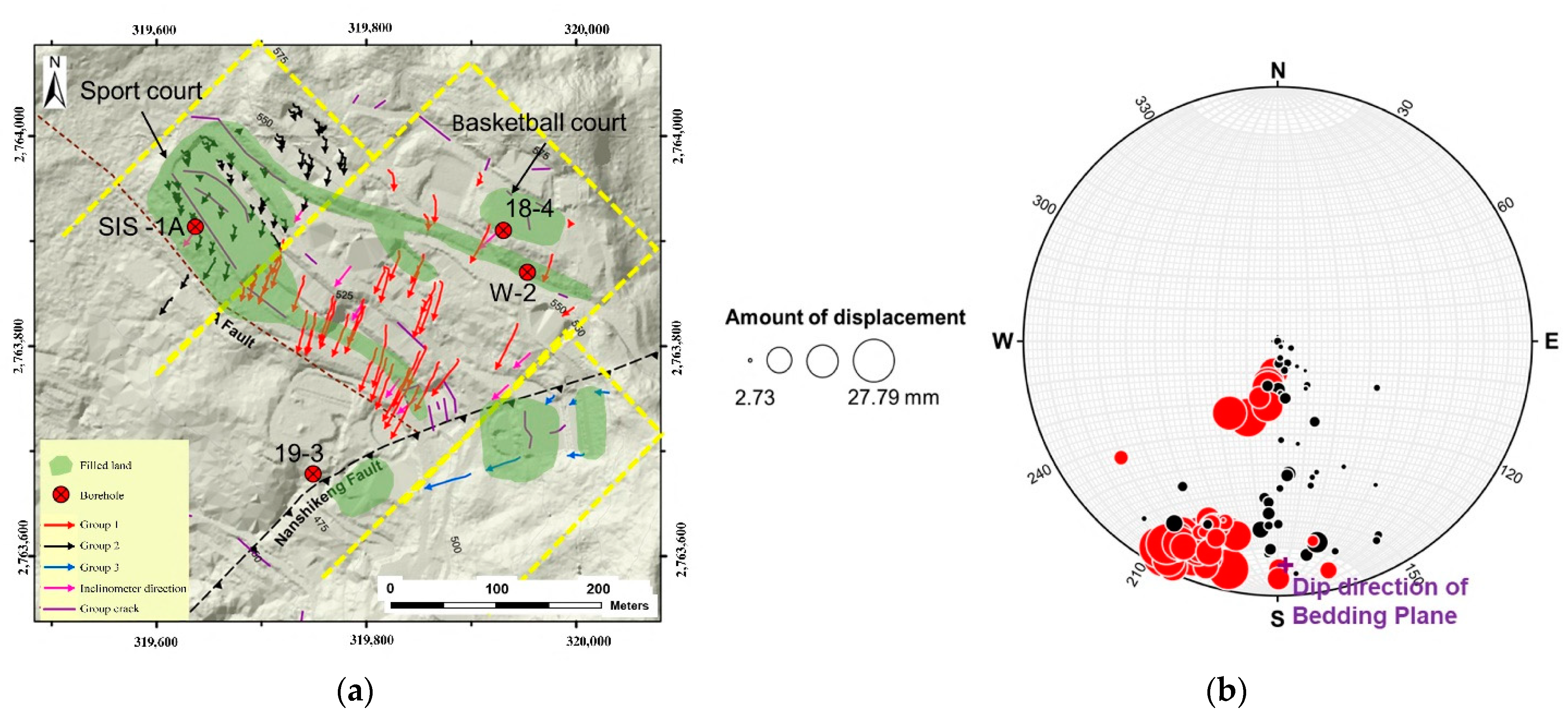
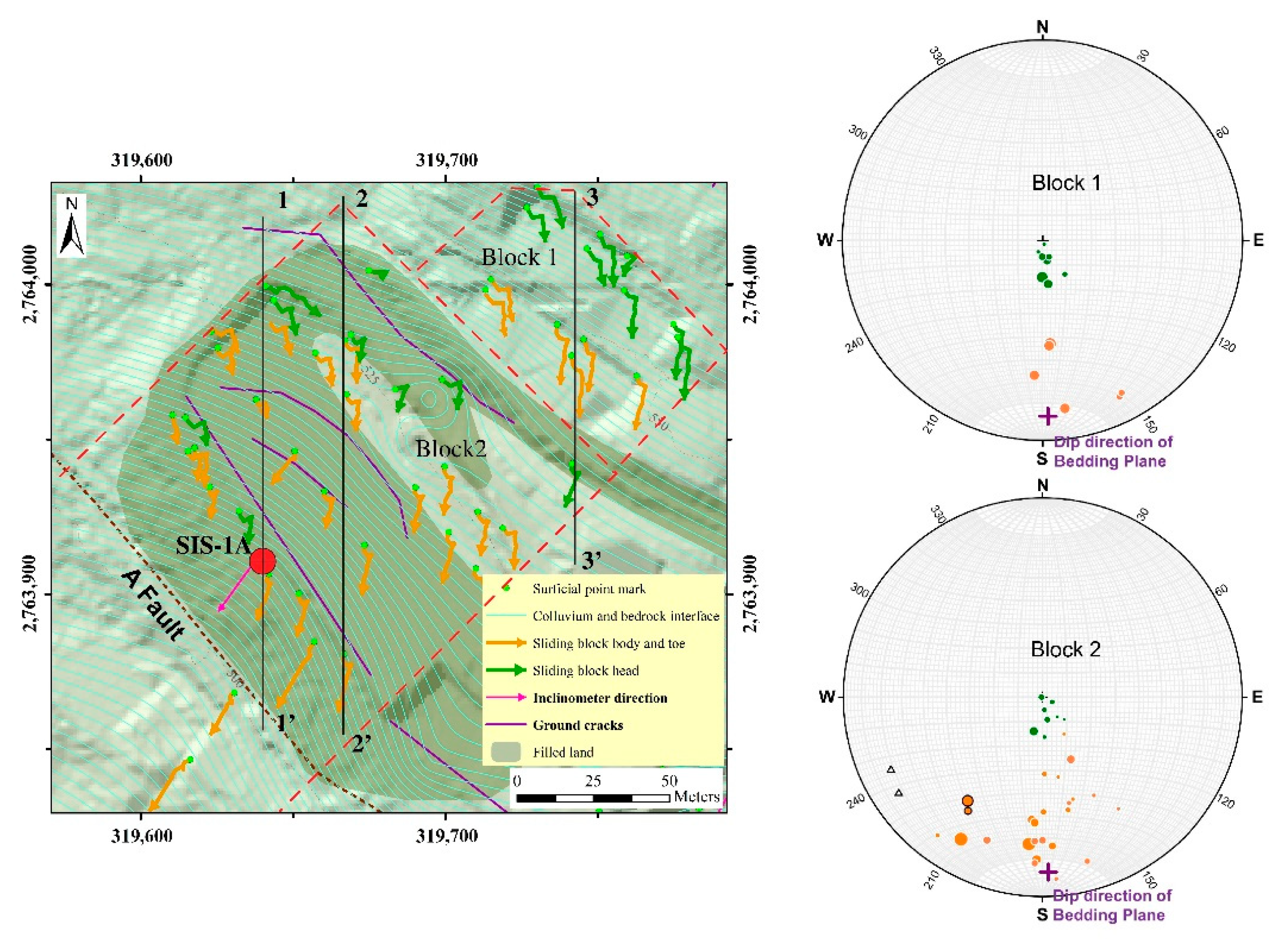
5.1.1. Surficial Displacement Interpretation
5.1.2. Sub-Surface Displacement Interpretation
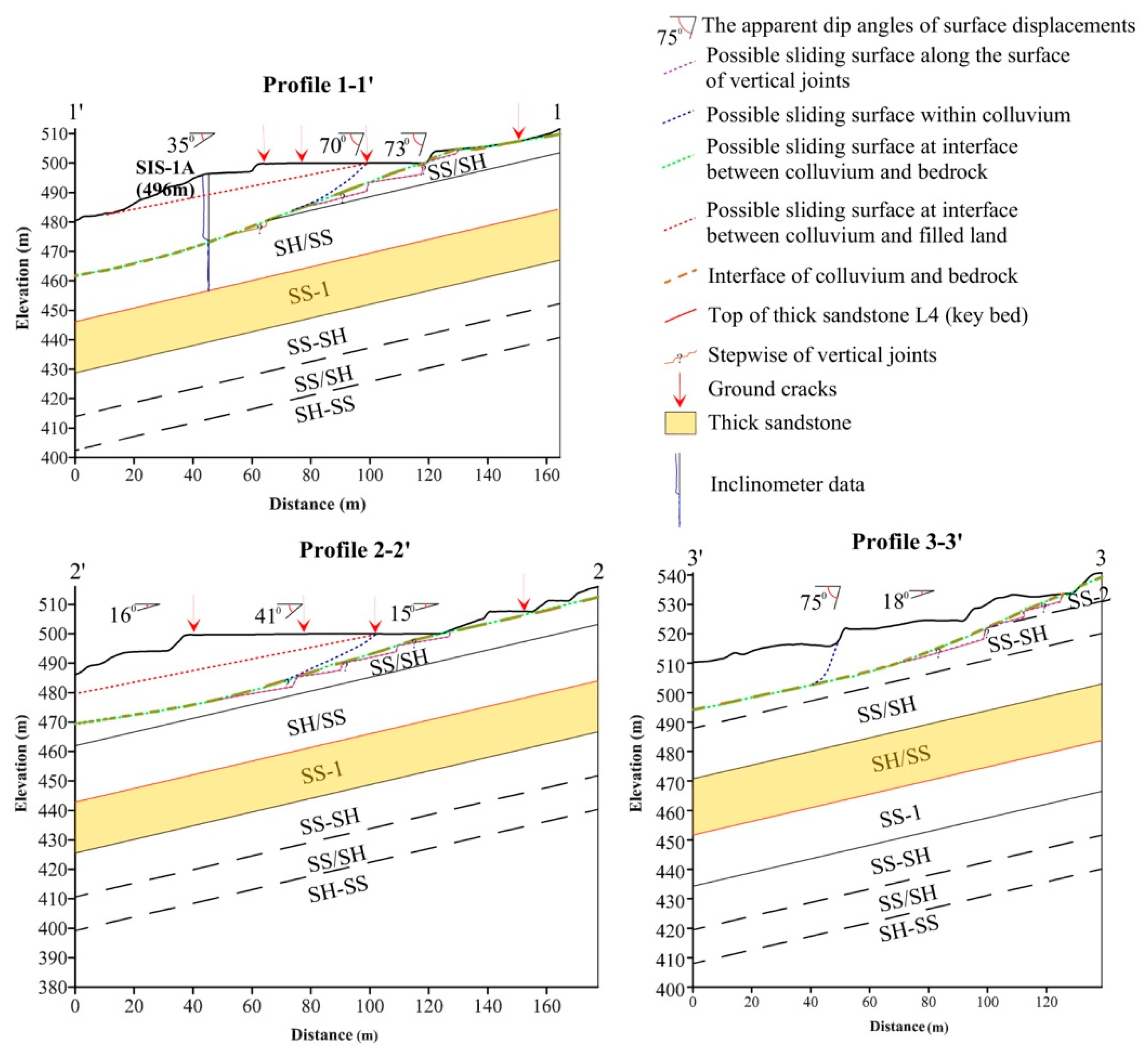
5.1.3. Slope Instability Mechanisms Based on 3D EGM
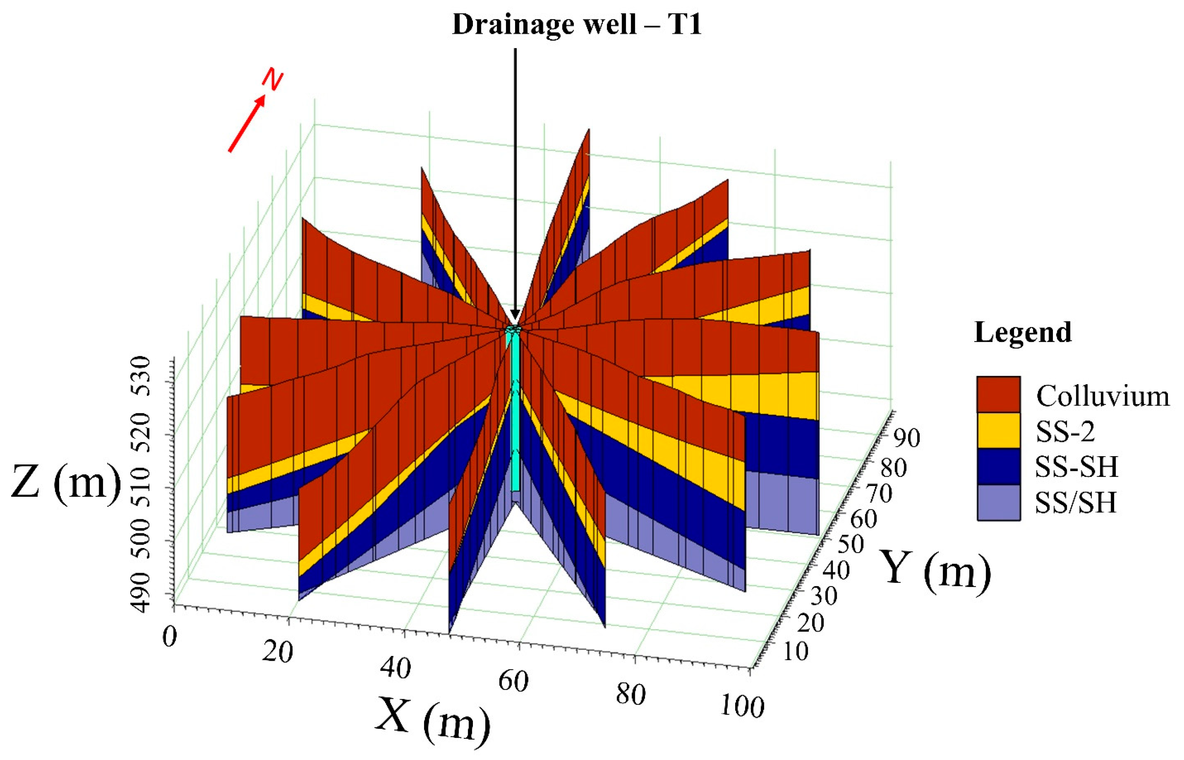
5.2. Application of the 3D EGM to Drainage Well Design
6. Conclusions
- (1)
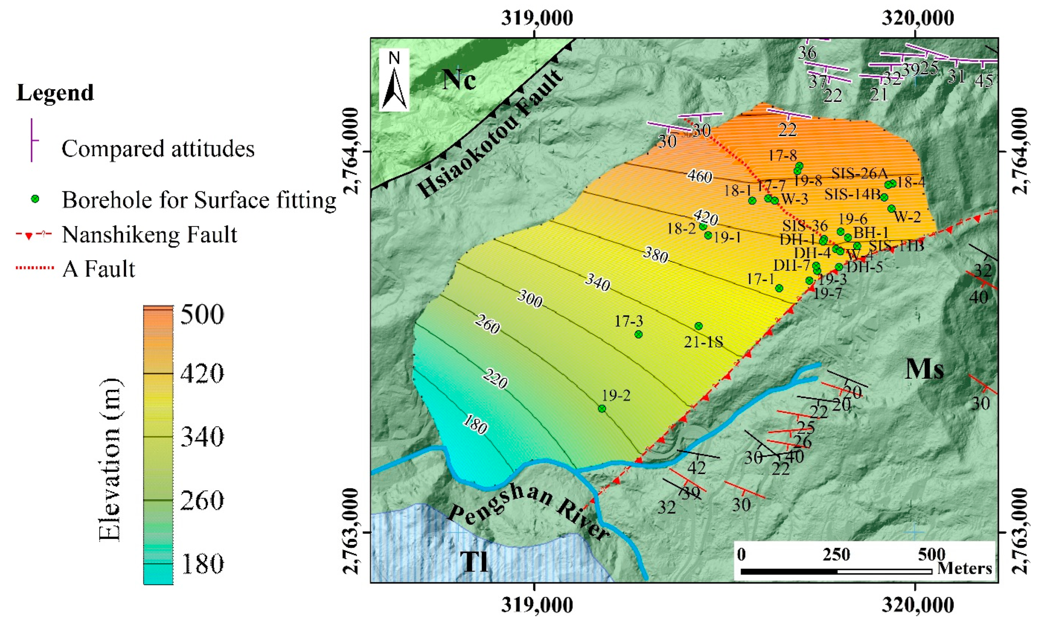
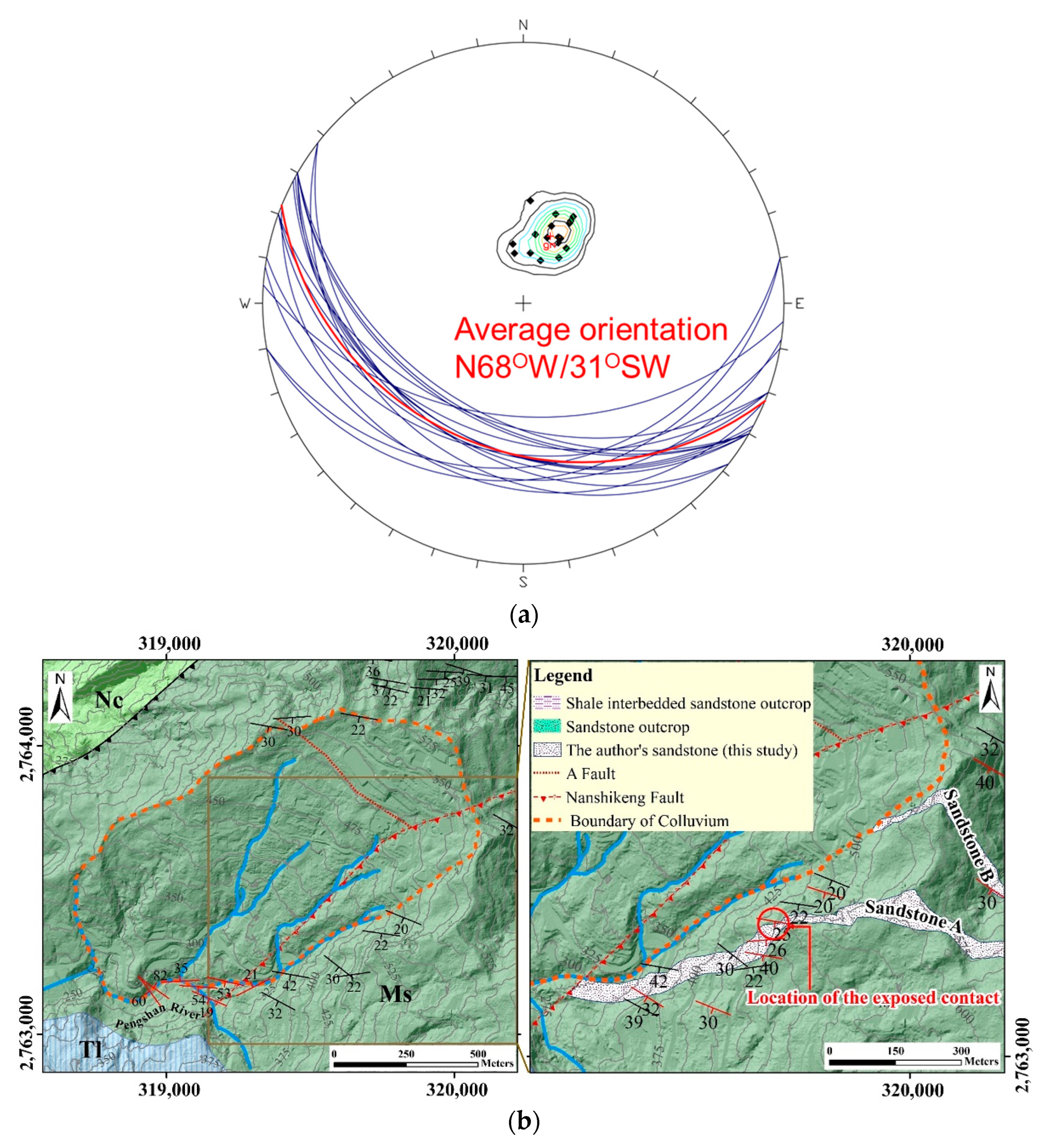
- The study area can be divided into three uniform geological zones belonging to the Mushan Formation. Two faults—the Nanshihkeng Fault and the A Fault—formed the boundaries of these three zones.
- (2)
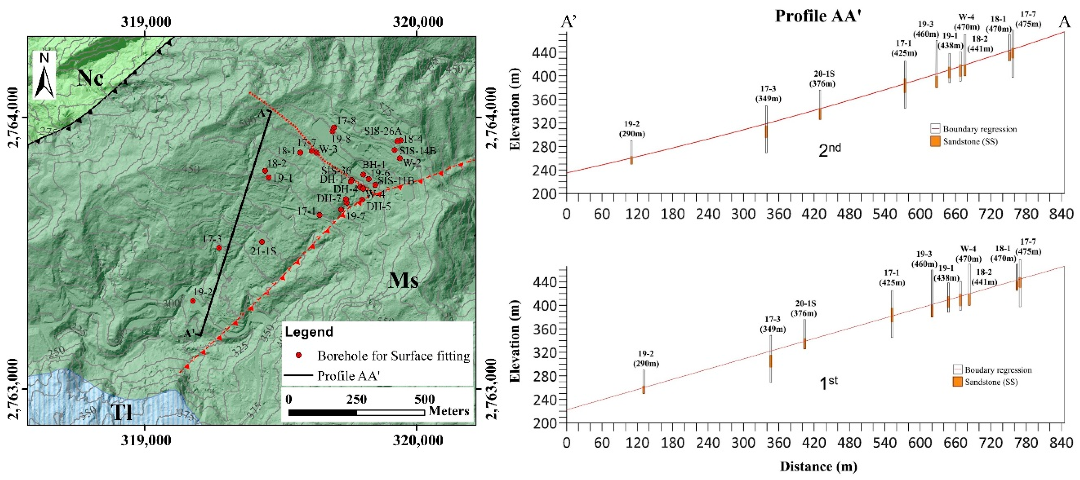
- The interpretation of the borehole cores provided a clear overall stratigraphy of the sedimentary rocks in the area. In particular, there were nine rock units that could be distinguished, including thick sandstone and a variable proportion of interbedded shale and sandstone for Zones 1 and 2, in the following order of stratigraphic history: L1 (SH/SS), L2 (SS/SH), L3 (SS-SH), L4 (SS-1), L5 (SH/SS), L6 (SS/SH), L7(SS-SH), L8 (SS-2), and L9 (SH/SS). The thick sandstone (L4) identified as the key bed is dominated by thick medium-grained whitish sandstone, intercalated with thin dark black shale layers dispersed in a few spots in the massive sandstone. The top boundary of this rock unit was observed from the borehole samples, following which this key bed was used for surface regression. In Zone 3, the spatial distribution of the two thick sandstones was proposed in the 3D EGM model as the consequence of outcrop field geology measurements and topographical analysis, by applying a high-resolution DEM.
- (3)
- Loose material covered the slope with varying thicknesses. It was most densely distributed in the southwestern slope, at approximately 50 m thick, and became thinner in the upper elevations along the mountain ridge. According to the topographical features, the colluvium may consist of material from various sources, such as ancient landslides or bedrock deterioration. The geometry of the bedding plane was calculated, based on its distribution, as a plane generally dipping 15° to the southwest.
- (4)
- Along with the 3D EGM, the structural contour map obtained by bedding surface fitting using a second-order model revealed that the geometry of the geological interface (i.e., the top surface of the key bed) gradually changes its direction and dip inclination (Zone 1). Even though the bedding in Zones 2 and 3 proposed in this study was found to be planar, its orientation changed significantly in space. Therefore, the underground information in both zones needs to be supplemented in future research.
- (5)
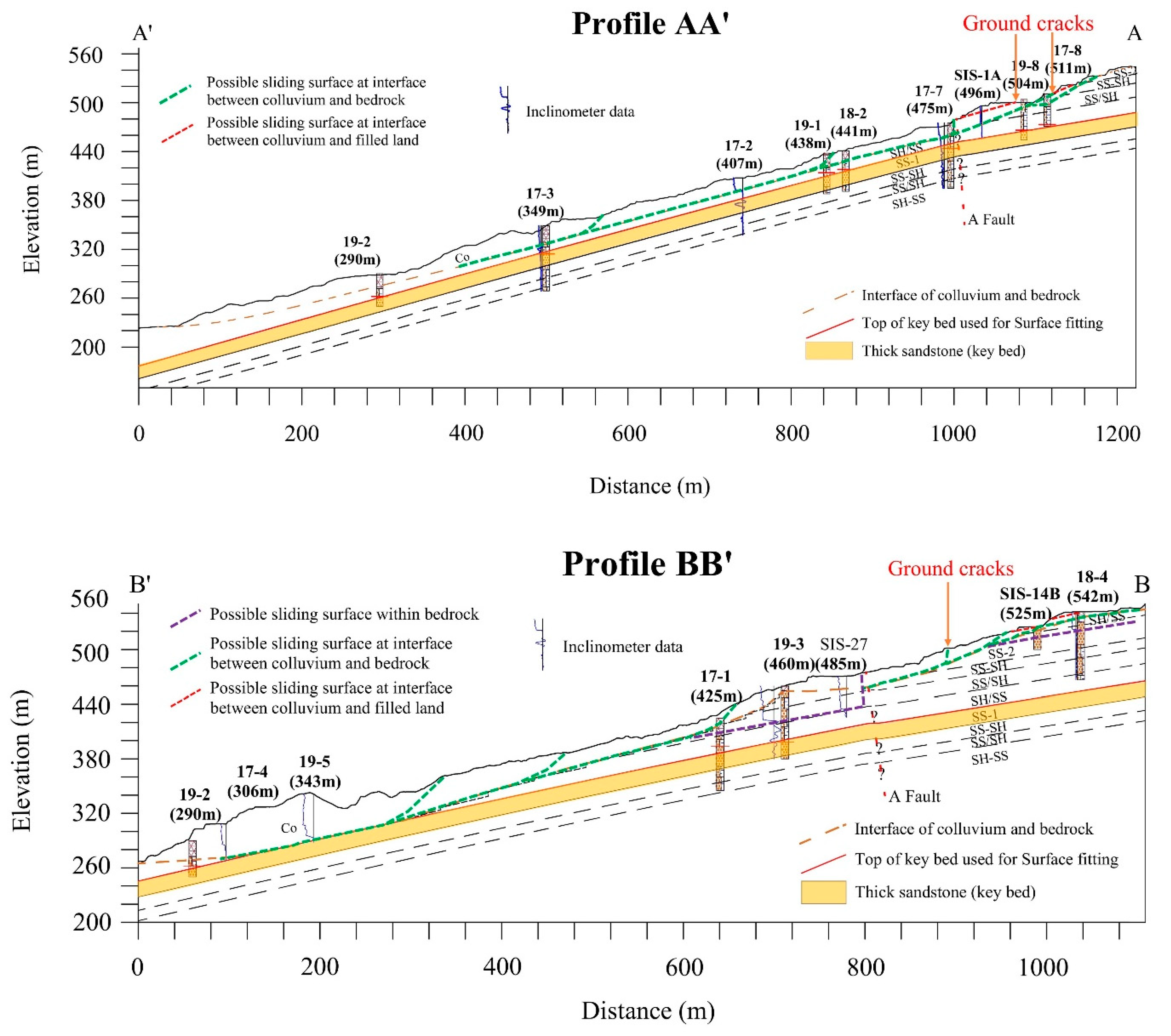
- The possibility of the future dip slope failure might be assessed through the use of a combination of surficial/underground monitoring. The geological model that incorporated the time-series of the displacement of the slope surface, revealed three sliding mechanism types. The first one comprises the sliding surface at the interface between the fill and the colluvium. The second one involves creeping on the contact surface between the colluvium and the underlying bedrock. The third mechanism is sliding occurring within the interlayer as a bedding plane. The development of deep-seated landslides through gully erosion was also proposed. However, the slope failure occurs only as local sliding and it is spatially very limited.
Author Contributions
Funding
Acknowledgments
Conflicts of Interest
References
- Parry, S.; Baynes, F.J.; Culshaw, M.G.; Eggers, M.; Keaton, J.F.; Lentfer, K.; Paul, D. Engineering geological models: An introduction: IAEG commission 25. Bull. Eng. Geol. Environ. 2014, 73, 689–706. [Google Scholar] [CrossRef]
- Fookes, P.G. Geology for engineers: The geological model, prediction and performance. Q. J. Eng. Geol. Hydrogeol. 1997, 30, 293–424. [Google Scholar] [CrossRef]
- Turner, A.K. Challenges and trends for geological modelling and visualisation. Bull. Eng. Geol. Environ. 2006, 65, 109–127. [Google Scholar] [CrossRef]
- Culshaw, M.G. From concept towards reality: Developing the attributed 3D geological model of the shallow subsurface. Q. J. Eng. Geol. Hydrogeol. 2005, 38, 231–284. [Google Scholar] [CrossRef]
- Caumon, G.; Collon-Drouaillet, P.L.C.D.; De Veslud, C.L.C.; Viseur, S.; Sausse, J. Surface-based 3D modeling of geological structures. Math. Geosci. 2009, 41, 927–945. [Google Scholar] [CrossRef]
- De Rienzo, F.; Oreste, P.; Pelizza, S. Subsurface geological-geotechnical modelling to sustain underground civil planning. Eng. Geol. 2008, 96, 187–204. [Google Scholar] [CrossRef]
- Lemon, A.M.; Jones, N.L. Building solid models from boreholes and user-defined cross-sections. Comput. Geosci. 2003, 29, 547–555. [Google Scholar] [CrossRef]
- Wu, Q.; Xu, H.; Zou, X. An effective method for 3D geological modeling with multi-source data integration. Comput. Geosci. 2005, 31, 35–43. [Google Scholar] [CrossRef]
- Zhu, L.; Zhang, C.; Li, M.; Pan, X.; Sun, J. Building 3D solid models of sedimentary stratigraphic systems from borehole data: An automatic method and case studies. Eng. Geol. 2012, 127, 1–13. [Google Scholar] [CrossRef]
- Kessler, H.; Mathers, S.; Sobisch, H.G. The capture and dissemination of integrated 3D geospatial knowledge at the British Geological Survey using GSI3D software and methodology. Comput. Geosci. 2009, 35, 1311–1321. [Google Scholar] [CrossRef]
- D’Agnese, F.A.; Faunt, C.C.; Turner, A.K.; Hill, M.C. Hydrogeologic Evaluation and Numerical Simulation of the Death Valley Regional Ground-Water Flow System, Nevada and California; US Department of the Interior; US Geological Survey: Denver, CO, USA, 1997; Volume 96, p. 4300.
- Logan, C.; Sharpe, D.R.; Russell, H.A. Regional Three-Dimensional Stratigraphic Modelling of the Oak Ridges Moraine Area, Southern Ontario; Natural Resources Canada; Geological Survey of Canada: Ottawa, ON, Canada, 2001.
- Tremblay, T.; Nastev, M.; Lamothe, M. Grid-based hydrostratigraphic 3D modelling of the Quaternary sequence in the Châteauguay River watershed, Quebec. Can. Water Resour. J. 2010, 35, 377–398. [Google Scholar] [CrossRef]
- Bistacchi, A.; Massironi, M.; Superchi, L.; Zorzi, L.; Francesca, R.; Giorgi, M.; Genevois, R. A 3D geological model of the 1963 Vajont landslide. Ital. J. Eng. Geol. Environ. 2013, 6, 531–539. [Google Scholar]
- Wang, J.; Schweizer, D.; Liu, Q.; Su, A.; Hu, X.; Blum, P. Three-dimensional landslide evolution model at the Yangtze River. Eng. Geol. 2021, 292, 106275. [Google Scholar] [CrossRef]
- Thierry, P.; Prunier-Leparmentier, A.M.; Lembezat, C.; Vanoudheusden, E.; Vernoux, J.F. 3D geological modelling at urban scale and mapping of ground movement susceptibility from gypsum dissolution: The Paris example (France). Eng. Geol. 2009, 105, 51–64. [Google Scholar] [CrossRef]
- Thapa, P.B. An approach towards integrated modelling of 3D geology and landslide susceptibility in the Lesser Himalaya of central Nepal. J. Nepal Geol. Soc. 2014, 47, 65–76. [Google Scholar] [CrossRef]
- Gu, T.; Wang, J.; Fu, X.; Liu, Y. GIS and limit equilibrium in the assessment of regional slope stability and mapping of landslide susceptibility. Bull. Eng. Geol. Environ. 2015, 74, 1105–1115. [Google Scholar] [CrossRef]
- Li, Z.; Zhang, F.; Gu, W.; Dong, M. The Niushou landslide in Nanjing City, Jiangsu Province of China: A slow-moving landslide triggered by rainfall. Landslides 2020, 17, 2603–2617. [Google Scholar] [CrossRef]
- Varnes, D.J. Slope Movements And Types And Processes. Landslides Analysis and Control. Transp. Res. Board Spec. Rep. 1978, 176, 11–33. [Google Scholar]
- Schulz, W.H.; McKenna, J.P.; Kibler, J.D.; Biavati, G. Relations between hydrology and velocity of a continuously moving landslide—Evidence of pore-pressure feedback regulating landslide motion? Landslides 2009, 6, 181–190. [Google Scholar] [CrossRef]
- Crozier, M.J. Landslide geomorphology: An argument for recognition, with examples from New Zealand. Geomorphology 2010, 120, 3–15. [Google Scholar] [CrossRef]
- Ross, M.; Parent, M.; Lefebvre, R. 3D geologic framework models for regional hydrogeology and land-use management: A case study from a Quaternary basin of southwestern Quebec, Canada. Hydrogeol. J. 2005, 13, 690–707. [Google Scholar] [CrossRef]
- Tang, W.; Tang, H. Grid-based three-dimensional geological models of the update method. In Proceedings of the 2011 International Conference on Multimedia Technology, IEEE, Hangzhou, China, 26–28 July 2011; pp. 1086–1089. [Google Scholar]
- Xie, M.; Esaki, T.; Qiu, C.; Wang, C. Geographical information system-based computational implementation and application of spatial three-dimensional slope stability analysis. Comput. Geotech. 2006, 33, 260–274. [Google Scholar] [CrossRef]
- Moore, I.D.; Turner, A.K.; Wilson, J.P.; Jenson, S.K.; Band, L.E. GIS and land-surface-subsurface process modeling. Environ. Modeling GIS 1993, 20, 196–230. [Google Scholar]
- Lindsay, M.D.; Aillères, L.; Jessell, M.W.; de Kemp, E.A.; Betts, P.G. Locating and quantifying geological uncertainty in three-dimensional models: Analysis of the Gippsland Basin, southeastern Australia. Tectonophysics 2012, 546, 10–27. [Google Scholar] [CrossRef]
- Jeng, C.J.; Sue, D.Z. Characteristics of ground motion and threshold values for colluvium slope displacement induced by heavy rainfall: A case study in northern Taiwan. Nat. Hazards Earth Syst. Sci. 2016, 16, 1309–1321. [Google Scholar] [CrossRef]
- Tseng, C.H.; Chan, Y.C.; Jeng, C.J.; Hsieh, Y.C. Slip monitoring of a dip-slope and runout simulation by the discrete element method: A case study at the Huafan University campus in northern Taiwan. Nat. Hazards 2017, 89, 1205–1225. [Google Scholar] [CrossRef]
- Tseng, C.H.; Chan, Y.C.; Jeng, C.J.; Rau, R.J.; Hsieh, Y.C. Deformation of landslide revealed by long-term surficial monitoring: A case study of slow movement of a dip slope in northern Taiwan. Eng. Geol. 2021, 284, 106020. [Google Scholar] [CrossRef]
- Central Geological Survey of Taiwan (CGS), 2000. Explanatory Text of the Geological Map of Taiwan, scale 1:50,000, Sheet 32. Hsintien. (In Chinese). Available online: https://twgeoref.moeacgs.gov.tw/GipOpenWeb/imgAction?f=/2000/20000110/EAB.PDF (accessed on 24 June 2022).
- Golden software, llc, Surfer 16. Golden software 2016, llc, Po box 281, Golden, CO 80402-0281 USA. Available online: https://www.goldensoftware.com/blog/surfer-16-is-here (accessed on 24 June 2022).
- Krumbein, W.C. Confidence intervals on low-order polynomial trend surfaces. J. Geophys. Res. 1963, 68, 5869–5878. [Google Scholar] [CrossRef]
- Chorley, R.J.; Haggett, P. Trend-surface mapping in geographical research. Trans. Inst. Br. Geogr. 1965, 37, 47–67. [Google Scholar] [CrossRef]
- Mei, S. Geologist-controlled trends versus computer-controlled trends: Introducing a high-resolution approach to subsurface structural mapping using well-log data, trend surface analysis, and geospatial analysis. Can. J. Earth Sci. 2009, 46, 309–329. [Google Scholar] [CrossRef]
- Bamisaiye, O.A. Subsurface mapping: Selection of best interpolation method for borehole data analysis. Spat. Inf. Res. 2018, 26, 261–269. [Google Scholar] [CrossRef]
- Cook, D.I.; Santi, P.M.; Higgins, J.D. 2007 AEG Student Professional Paper: Graduate Division: Horizontal Landslide Drain Design: State of the Art and Suggested Improvements. Environ. Eng. Geosci. 2008, 14, 241–250. [Google Scholar] [CrossRef]


| Borehole | X | Y | Z | Error | |
|---|---|---|---|---|---|
| 2nd | 1st | ||||
| W-4 | 319,803.7 | 2,763,737.5 | 413 | 4.10 | 7.00 |
| 19-7 | 319,722.7 | 2,763,660.8 | 390.6 | 5.46 | 2.20 |
| 19-3 | 319,743.2 | 2,763,686.7 | 399 | 3.95 | 2.53 |
| DH-5 | 319,800.2 | 2,763,697.0 | 411 | −3.14 | 2.79 |
| DH-7 | 319,740.0 | 2,763,699.7 | 403.8 | 1.95 | 1.23 |
| DH-4 | 319,792.5 | 2,763,743.6 | 422 | −3.75 | −0.98 |
| DH-1 | 319,758.2 | 2,763,763.9 | 423 | −1.00 | 1.57 |
| SIS-36 | 319,761 | 2,763,769.8 | 427 | −3.40 | −0.53 |
| 18-2 | 319,443.5 | 2,763,803.5 | 418 | −2.21 | −2.63 |
| 19-1 | 319,456.7 | 2,763,780.4 | 414 | −4.36 | −4.38 |
| 18-1 | 319,572.3 | 2,763,871.3 | 440 | 4.90 | 3.16 |
| 17-7 | 319,614.1 | 2,763,867.3 | 444.4 | 1.03 | 0.32 |
| 17-3 | 319,273.8 | 2,763,519.9 | 314.3 | 4.06 | 8.91 |
| 17-1 | 319,643.2 | 2,763,641.1 | 394 | −7.46 | −12.01 |
| 19-2 | 319,177.7 | 2,763,324.5 | 262 | −1.79 | −0.88 |
| 21-1S | 319,431.5 | 2,763,541.8 | 342.5 | 1.58 | −2.70 |
| Borehole | X | Y | Z | Error |
|---|---|---|---|---|
| W-3 | 319,631.7 | 2,763,871.4 | 443.8 | 3.68 |
| 17-8 | 319,696.5 | 2,763,972 | 472.8 | −2.5 |
| 19-8 | 319,691.3 | 2,763,949.3 | 466.2 | −1.22 |
| BH-1 | 319,823.9 | 2,763,774.3 | 428.6 | −5.38 |
| 19-6 | 319,804.5 | 2,763,789.9 | 424.8 | 2.21 |
| W-2 | 319,938.1 | 2,763,849.8 | 440.3 | −0.67 |
| 18-4 | 319,941.3 | 2,763,915.9 | 452.8 | 2.11 |
| SIS-14B | 319,919.3 | 2,763,880 | 446.9 | −0.01 |
| SIS-26A | 319,929.6 | 2,763,913 | 453.7 | 0.7 |
| SIS-11B | 319,848 | 2,763,752 | 416.7 | 1.1 |
Publisher’s Note: MDPI stays neutral with regard to jurisdictional claims in published maps and institutional affiliations. |
© 2022 by the authors. Licensee MDPI, Basel, Switzerland. This article is an open access article distributed under the terms and conditions of the Creative Commons Attribution (CC BY) license (https://creativecommons.org/licenses/by/4.0/).
Share and Cite
Nguyễn, T.-T.; Dong, J.-J.; Tseng, C.-H.; Baroň, I.; Chen, C.-W.; Pai, C.-C. Three-Dimensional Engineering Geological Model and Its Applications for a Landslide Site: Combination of Grid- and Vector-Based Methods. Water 2022, 14, 2941. https://doi.org/10.3390/w14192941
Nguyễn T-T, Dong J-J, Tseng C-H, Baroň I, Chen C-W, Pai C-C. Three-Dimensional Engineering Geological Model and Its Applications for a Landslide Site: Combination of Grid- and Vector-Based Methods. Water. 2022; 14(19):2941. https://doi.org/10.3390/w14192941
Chicago/Turabian StyleNguyễn, Thanh-Tùng, Jia-Jyun Dong, Chia-Han Tseng, Ivo Baroň, Chao-Wei Chen, and Chao-Chin Pai. 2022. "Three-Dimensional Engineering Geological Model and Its Applications for a Landslide Site: Combination of Grid- and Vector-Based Methods" Water 14, no. 19: 2941. https://doi.org/10.3390/w14192941
APA StyleNguyễn, T.-T., Dong, J.-J., Tseng, C.-H., Baroň, I., Chen, C.-W., & Pai, C.-C. (2022). Three-Dimensional Engineering Geological Model and Its Applications for a Landslide Site: Combination of Grid- and Vector-Based Methods. Water, 14(19), 2941. https://doi.org/10.3390/w14192941