
Effectiveness of Biomass/Abundance Comparison (ABC) Models in Assessing the Response of Hyporheic Assemblages to Ammonium Contamination

 ,
,  ,
, 
Abstract
:
1. Introduction
2. Materials and Methods
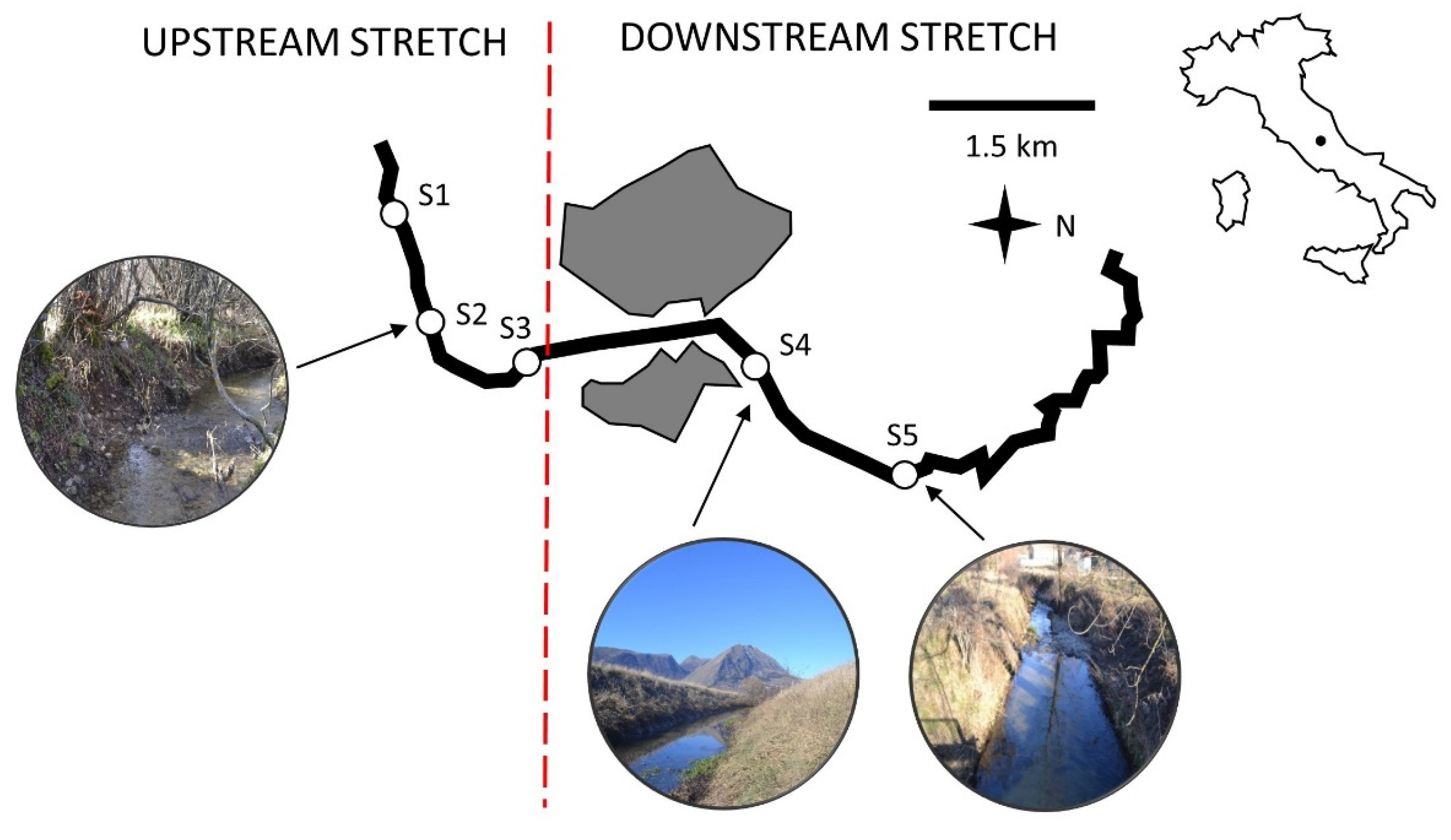
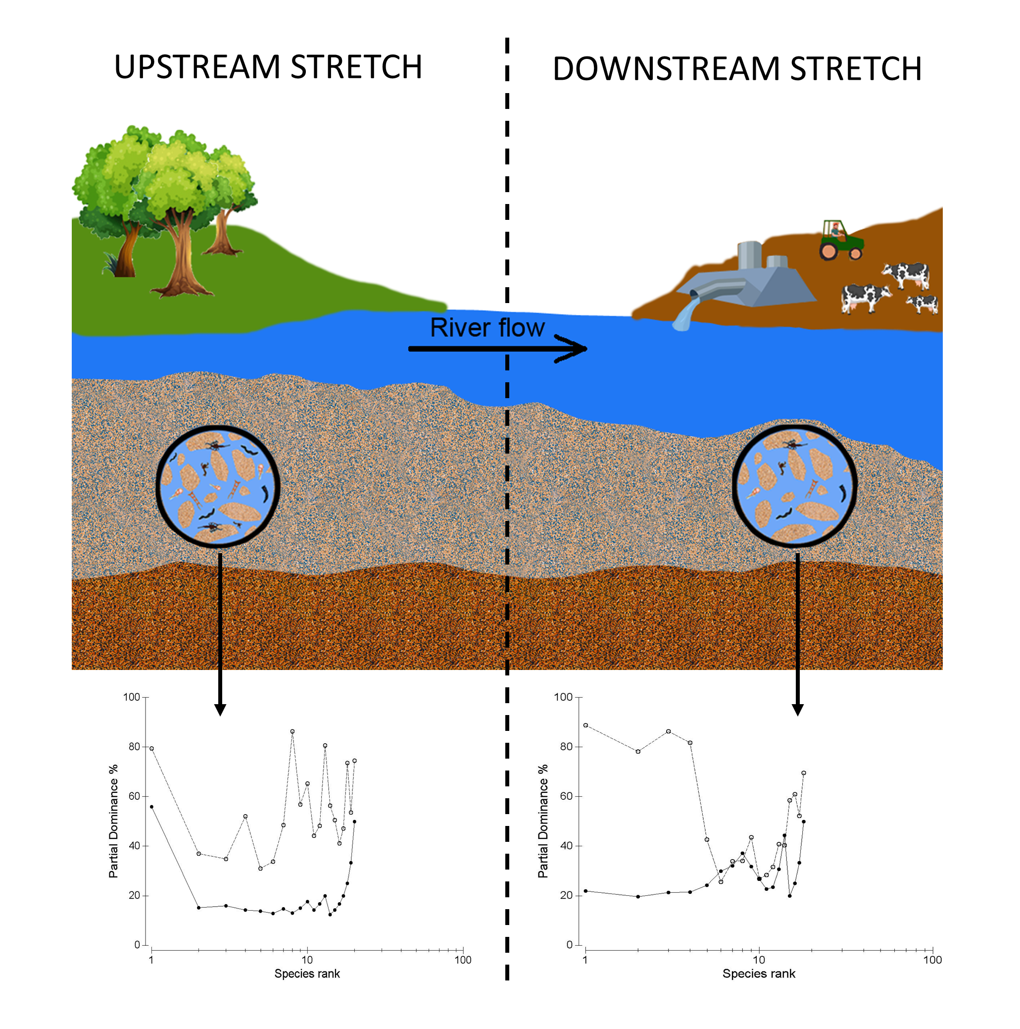
2.1. Study Area
2.2. Sample Collection and Processing
2.3. ABC Models
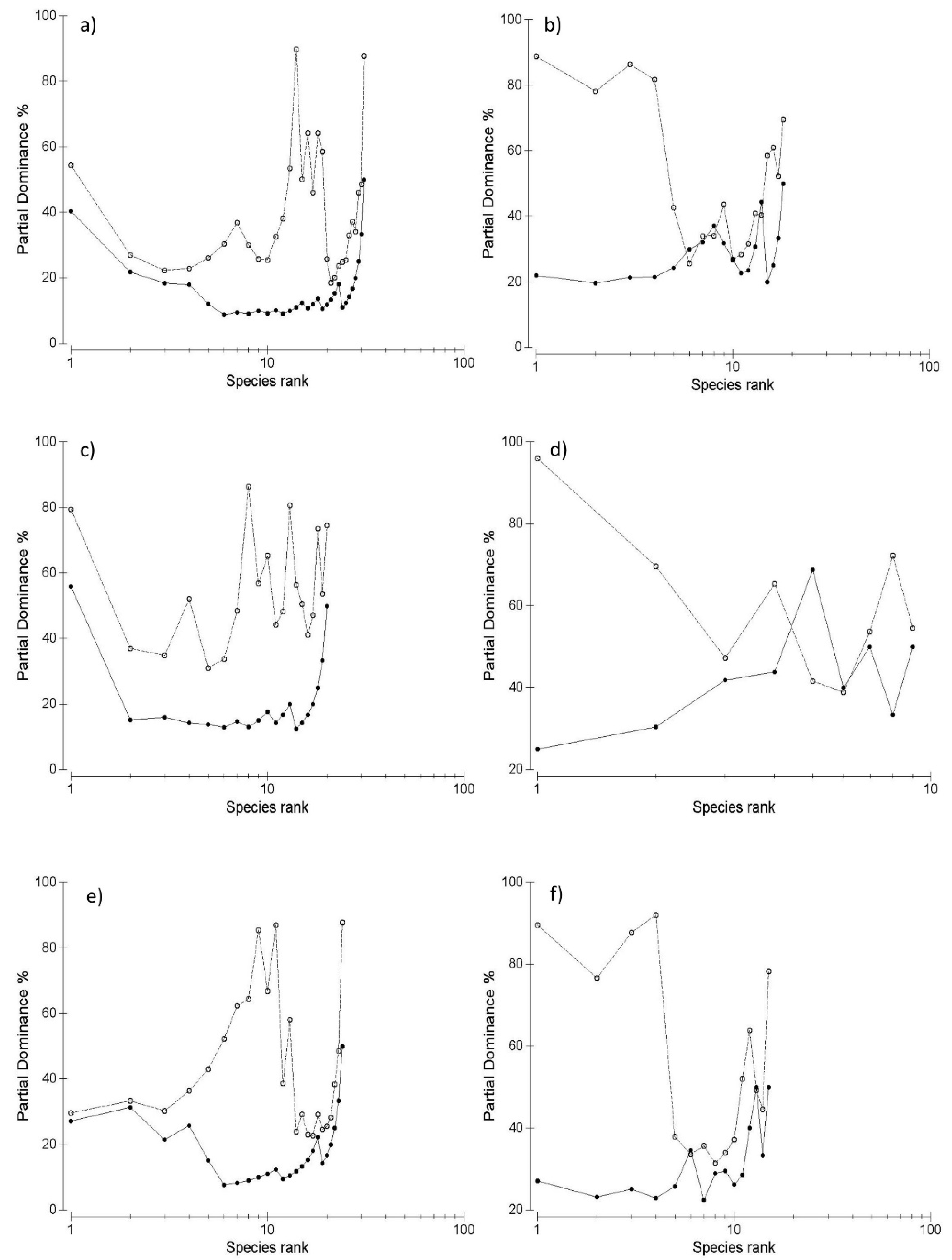
3. Results
4. Discussion
5. Conclusions
Supplementary Materials
Author Contributions
Funding
Data Availability Statement
Acknowledgments
Conflicts of Interest
References
- Warwick, R.M. A new method for detecting pollution effects on marine macrobenthic communities. Mar. Biol. 1986, 92, 557–562. [Google Scholar] [CrossRef]
- Lambshead, P.J.D.; Platt, H.M.; Shaw, K.M. The detection of differences among assemblages of marine benthic species based on an assessment of dominance and diversity. J. Nat. Hist. 1983, 17, 859–874. [Google Scholar] [CrossRef]
- Clarke, K.R. Comparisons of dominance curves. J. Exp. Mar. Biol. Ecol. 1990, 138, 143–157. [Google Scholar] [CrossRef]
- Clarke, K.R.; Gorley, R.N. PRIMER v7: User Manual/Tutorial.; PRIMER-E Ltd.: Plymouth, UK, 2015. [Google Scholar]
- Dauer, D.M.; Luckenbach, M.W.; Rodi, A.J. Abundance biomass comparison (ABC method): Effects of an estuarine gradient, anoxic/hypoxic events and contaminated sediments. Mar. Biol. 1993, 116, 507–518. [Google Scholar] [CrossRef]
- Warwick, R.M.; Pearson, T.H. Detection of pollution effects on marine macrobenthos: Further evaluation of the species abundance/biomass method. Mar. Biol. 1987, 95, 193–200. [Google Scholar] [CrossRef]
- Warwick, R.M.; Clarke, K.R. Relearning the ABC: Taxonomic changes and abundance/biomass relationships in disturbed benthic communities. Mar. Biol. 1994, 118, 739–744. [Google Scholar] [CrossRef]
- Xu, S.; Guo, J.; Liu, Y.; Fan, J.; Xiao, Y.; Xu, Y.; Li, C.; Barati, B. Evaluation of Fish Communities in Daya Bay Using Biomass Size Spectrum and ABC Curve. Front. Environ. Sci. 2021, 9, 663169. [Google Scholar] [CrossRef]
- Meire, P.M.; Dereu, J. Use of the abundance/biomass comparison method for detecting environmental stress: Some considerations based on intertidal macrozoobenthos and bird communities. J. Appl. Ecol. 1990, 27(1), 210–223. [Google Scholar] [CrossRef]
- Smith, W.H.; Rissler, L.J. Quantifying disturbance in terrestrial communities: Abundance–biomass comparisons of herpetofauna closely track forest succession. Restor. Ecol. 2010, 18, 195–204. [Google Scholar] [CrossRef]
- Woessner, W.W. Chapter 8—Hyporheic Zones. In Methods in Stream Ecology, 3rd ed.; Hauer, R.F., Lamberti, G.A., Eds.; Academic Press: Cambridge, MA, USA, 2017; Volume 1, pp. 129–157. [Google Scholar]
- Brunke, M.; Gonser, T.O.M. The ecological significance of exchange processes between rivers and groundwater. Freshwat. Biol. 1997, 37, 1–33. [Google Scholar] [CrossRef] [Green Version]
- Boulton, A.J.; Datry, T.; Kasahara, T.; Mutz, M.; Stanford, J.A. Ecology and management of the hyporheic zone: Stream–groundwater interactions of running waters and their floodplains. J. N. Am. Benthol. Soc. 2010, 29, 26–40. [Google Scholar] [CrossRef]
- Williams, D.D.; Febria, C.M.; Wong, J.C. Ecotonal and other properties of the hyporheic zone. Fundam. Appl. Limnol. 2010, 176, 349. [Google Scholar] [CrossRef]
- Peralta-Maraver, I.; Galloway, J.; Posselt, M.; Arnon, S.; Reiss, J.; Lewandowski, J.; Robertson, A.L. Environmental filtering and community delineation in the streambed ecotone. Sci. Rep. 2018, 8, 1–11. [Google Scholar] [CrossRef] [PubMed]
- Storey, R.G.; Fulthorpe, R.R.; Williams, D.D. Perspectives and predictions on the microbial ecology of the hyporheic zone. Freshwat. Biol. 1999, 41, 119–130. [Google Scholar] [CrossRef]
- Hakenkamp, C.C.; Palmer, M.A. The ecology of hyporheic meiofauna. In Streams and Ground Waters; Jones, J.B., Mulholland, P.J., Eds.; Elsevier: Amsterdam, The Netherlands, 2000; pp. 307–336. [Google Scholar] [CrossRef]
- Wood, P.J.; Boulton, A.J.; Little, S.; Stubbington, R. Is the hyporheic zone a refugium for macroinvertebrates during severe low flow conditions? Fund. Appl. Limnol. 2010, 176, 377–390. [Google Scholar] [CrossRef]
- Kawanishi, R.; Inoue, M.; Dohi, R.; Fujii, A.; Miyake, Y. The role of the hyporheic zone for a benthic fish in an intermittent river: A refuge, not a graveyard. Aquat. Sci. 2013, 75, 425–431. [Google Scholar] [CrossRef]
- Lewandowski, J.; Arnon, S.; Banks, E.; Batelaan, O.; Betterle, A.; Broecker, T.; Coll, C.; Drummond, J.D.; Gaona Garcia, J.; Galloway, J.; et al. Is the hyporheic zone relevant beyond the scientific community? Water 2019, 11, 2230. [Google Scholar] [CrossRef]
- Di Lorenzo, T.; Fiasca, B.; Di Cicco, M.; Cifoni, M.; Galassi, D.M.P. Taxonomic and functional trait variation along a gradient of ammonium contamination in the hyporheic zone of a Mediterranean stream. Ecol. Indic. 2021, 132, 108268. [Google Scholar] [CrossRef]
- Anderson, M.J. A new method for non-parametric multivariate analysis of variance. Austral. Ecol. 2001, 26, 32–46. [Google Scholar] [CrossRef]
- Anderson, M.J.; Robinson, J. Permutation tests for linear models. Aust. N. Z. J. Stat. 2001, 43, 7588. [Google Scholar] [CrossRef]
- Di Marzio, W.D.; Cifoni, M.; Sáenz, M.E.; Galassi, D.M.P.; Di Lorenzo, T. The ecotoxicity of binary mixtures of Imazamox and ionized ammonia on freshwater copepods: Implications for environmental risk assessment in groundwater bodies. Ecotoxicol. Environ. Safe. 2018, 149, 72–79. [Google Scholar] [CrossRef] [PubMed]
- Di Marzio, W.D.; Castaldo, D.; Pantani, C.; Di Cioccio, A.; Di Lorenzo, T.; Sáenz, M.E.; Galassi, D.M.P. Relative sensitivity of hyporheic copepods to chemicals. Bull. Environ. Contam. Toxicol. 2009, 82, 488–491. [Google Scholar] [CrossRef]
- Di Marzio, W.D.; Castaldo, D.; Di Lorenzo, T.; Di Cioccio, A.; Sáenz, M.E.; Galassi, D.M.P. Developmental endpoints of chronic exposure to suspected endocrine-disrupting chemicals on benthic and hyporheic freshwater copepods. Ecotoxicol. Environ. Safe. 2013, 96, 86–92. [Google Scholar] [CrossRef] [PubMed]
- Di Lorenzo, T.; Di Marzio, W.D.; Cifoni, M.; Fiasca, B.; Baratti, M.; Sáenz, M.E.; Galassi, D.M.P. Temperature effect on the sensitivity of the copepod Eucyclops serrulatus (Crustacea, Copepoda, Cyclopoida) to agricultural pollutants in the hyporheic zone. Curr. Zool. 2015, 61, 629–640. [Google Scholar] [CrossRef]
- Di Lorenzo, T.; Cifoni, M.; Lombardo, P.; Fiasca, B.; Galassi, D.M.P. Ammonium threshold values for groundwater quality in the EU may not protect groundwater fauna: Evidence from an alluvial aquifer in Italy. Hydrobiologia 2015, 743, 139–150. [Google Scholar] [CrossRef]
- Di Lorenzo, T.; Cannicci, S.; Spigoli, D.; Cifoni, M.; Baratti, M.; Galassi, D.M.P. Bioenergetic cost of living in polluted freshwater bodies: Respiration rates of the cyclopoid Eucyclops serrulatus under ammonia-N exposures. Fundam. Appl. Limnol. 2016, 18, 147–156. [Google Scholar] [CrossRef]
- Arenas-Sánchez, A.; Dolédec, S.; Vighi, M.; Rico, A. Effects of anthropogenic pollution and hydrological variation on macroinvertebrates in Mediterranean rivers: A case-study in the upper Tagus river basin (Spain). Sci. Total Environ. 2021, 766, 144044. [Google Scholar] [CrossRef]
- Scorzini, A.R.; Leopardi, M. River basin planning: From qualitative to quantitative flood risk assessment: The case of Abruzzo Region (central Italy). Nat. Hazards 2017, 88, 71–93. [Google Scholar] [CrossRef]
- Wentworth, C.K. A scale of grade and class terms for clastic sediments. J. Geol. 1992, 30, 377–392. [Google Scholar] [CrossRef]
- Malard, F.; Dole-Olivier, M.-J.; Mathieu, J.; Stoch, F. Sampling manual for the assessment of regional groundwater biodiversity. In European Project PASCALIS (Protocols for the Assessment and Conservation of Aquatic Life in the Subsurface); Fift Framework Programme Key Action 2: Global Change, Climate and Biodiversity 2.2.3 Assessing and Conserving Bio-diversity Contract n◦ EVK2–CT–2001–00121; Available online: https://www.researchgate.net/publication/267567541_Sampling_Manual_for_the_Assessment_of_Regional_Groundwater_Biodiversity#fullTextFileContent (accessed on 12 July 2022).
- Mugnai, R.; Sousa, F.N.F.; Di Lorenzo, T. Monitoring hyporheic habitats: Techniques for unclogging minipiezometers. Pan-Am. J. Aquat. Sci. 2015, 10, 168171. [Google Scholar]
- Bou, C.; Rouch, R. Un nouveau champ de recherches sur le faune aquatique souterraine. C. R. Acad. Sci. Paris 1967, 265, 369370. [Google Scholar]
- Dussart, B.H. Les copépodes des Eaux Continentales d’Europe Occidentale, Tome I: Calanoïdes et Harpacticoïdes; Boubée et Cie: Paris, France, 1967; pp. 1–500. [Google Scholar]
- Dussart, B.H. Les Copépodes des Eaux Continentales d’Europe Occidentale, Tome 2: Cyclopöides et Biologie; Boubée et Cie: Paris, France, 1969; pp. 1–292. [Google Scholar]
- Campaioli, S.; Ghetti, P.F.; Minelli, A.; Ruffo, S. Manuale per il riconoscimento dei macroinvertebrati delle Acque Dolci Italiane. Volumes I & II; Provincia Autonoma di Trento: Trento, Italy, 1994; pp. 1–484. [Google Scholar]
- Di Sabatino, A.; Boggero, A.; Miccoli, F.P.; Cicolani, B. Diversity, distribution and ecology of water mites (Acari: Hydrachnidia and Halacaridae) in high Alpine lakes (Central Alps, Italy). Exp. Appl. Acarol. 2004, 34, 199–210. [Google Scholar] [CrossRef]
- Dussart, B.; Defaye, D. World Directory of Crustacea Copepoda of Inland Waters. II—Cyclopiformes; Backhuys Publishers: Leiden, The Netherlands, 2006; pp. 1–354. [Google Scholar]
- Puente, A.; Diaz, R.J. Is it possible to assess the ecological status of highly stressed natural estuarine environments using macroinvertebrates indices? Mar. Pollut. Bull. 2008, 56, 1880–1889. [Google Scholar] [CrossRef] [PubMed]
- Reiss, J.; Schmid-Araya, J.M. Existing in plenty: Abundance, biomass and diversity of ciliates and meiofauna in small streams. Freshw. Biol. 2008, 53, 652–668. [Google Scholar] [CrossRef]
- European Commission. Water Framework Directive 2000/60/EC of the European Parliament and of the Council establishing a framework for Community action in the field of water policy. OJ 2000, 327, 1–73. [Google Scholar]
- Woodward, G.; Bonada, N.; Feeley, H.B.; Giller, P.S. Resilience of a stream community to extreme climatic events and long-term recovery from a catastrophic flood. Freshwat. Biol. 2015, 60, 2497–2510. [Google Scholar] [CrossRef]
- Iliopoulou-Georgudaki, J.; Kantzaris, V.; Katharios, P.; Kaspiris, P.; Georgiadis, T.; Montesantou, B. An application of different bioindicators for assessing water quality: A case study in the rivers Alfeios and Pineios (Peloponnisos, Greece). Ecol. Indic. 2003, 2, 345360. [Google Scholar] [CrossRef]
- Radojević, A.; Mirčić, D.; Živić, M.; Perić Mataruga, V.; Božanić, M.; Stojanović, K.; Lukicic, J.; Živić, I. Influence of trout farm effluents on selected oxidative stress biomarkers in larvae of Ecdyonurus venosus (Ephemeroptera, Heptageniidae). Arch. Biol. Sci. 2019, 71, 225–233. [Google Scholar] [CrossRef]
- Burton, S.M.; Rundle, S.D.; Jones, M.B. The relationship between trace metal contamination and stream meiofauna. Environ. Pollut. 2001, 111, 159–167. [Google Scholar] [CrossRef]
- Beketov, M. Different sensitivity of mayflies (Insecta, Ephemeroptera) to ammonia, nitrite and nitrate: Linkage between experimental and observational data. Hydrobiologia 2004, 528, 209–216. [Google Scholar] [CrossRef]
- Pacioglu, O.; Pârvulescu, L. The chalk hyporheic zone: A true ecotone? Hydrobiologia 2017, 790, 1–12. [Google Scholar] [CrossRef]
- Iepure, S.; Martinez-Hernandez, V.; Herrera, S.; Rasines-Ladero, R.; de Bustamante, I. Response of microcrustacean communities from the surface—groundwater interface to water contamination in urban river system of the Jarama basin (central Spain). Environ. Sci. Pollut. Res. 2013, 20, 5813–5826. [Google Scholar] [CrossRef]
- Notenboom, J.; Plénet, S.; Turquin, M.-J. Groundwater contamination and its impact on groundwater animals and ecosystems. In Groundwater ecology; Gibert, J., Danielopol, D.L., Standford, J.A., Eds.; Academic Press: San Diego, CA, USA, 1994; pp. 477–504. [Google Scholar]
- Lafont, M.; Vivier, A. Oligochaete assemblages in the hyporheic zone and coarse surface sediments: Their importance for understanding of ecological functioning of watercourses. Hydrobiologia 1998, 334, 147–155. [Google Scholar] [CrossRef]
- Moldovan, O.T.; Meleg, I.; Levei, E.; Terente, M. A simple method for assessing biotic indicators and predicting biodiversity in the hyporheic zone of a river polluted with metals. Ecol. Indic. 2013, 24, 412–420. [Google Scholar] [CrossRef]
- Green, R.H. Sampling Design and Statistical Methods for Environmental Biologists; John Wiley & Sons: New York, NY, USA, 1979; pp. 1–272. [Google Scholar]


| Taxon | Abb | Abb_W | Abb_S | Bio | Bio_W | Bio_S |
|---|---|---|---|---|---|---|
| Leuctra fusca fusca (Linnaeus, 1758) | 13.0 | 1.5 | 22.8 | 20.9 | 16.4 | 44.0 |
| Protonemura salfii (Aubert, 1954) | 0.3 | 0.0 | 0.6 | 3.6 | 0.6 | 8.9 |
| Siphlonurus lacustris Eaton, 1870 | 0.7 | 0.0 | 1.3 | 7.1 | 0.0 | 17.4 |
| Ecdyonurus gr. venosus | 0.7 | 0.7 | 0.6 | 52.3 | 71.9 | 0.1 |
| Baetis sp. | 0.3 | 0.0 | 0.6 | 1.9 | 0.0 | 4.6 |
| Rhyacophila foliacea Moretti, 1981 | 0.7 | 0.0 | 1.3 | 0.4 | 0.0 | 1.0 |
| Elmidae | 3.8 | 6.0 | 1.9 | 0.8 | 0.8 | 0.5 |
| Athericidae | 1.4 | 0.7 | 1.9 | 1.1 | 0.1 | 2.8 |
| Simuliidae | 0.3 | 0.7 | 0.0 | 5.0 | 6.9 | 0.0 |
| Limoniidae | 0.3 | 0.7 | 0.0 | 0.6 | 0.9 | 0.0 |
| Chironomidae | 40.4 | 56.0 | 27.2 | 5.7 | 4.1 | 6.7 |
| Ceratopogonidae | 0.3 | 0.7 | 0.0 | 0.5 | 0.7 | 0.0 |
| Gammarus elvirae Iannilli & Ruffo, 2002 | 1.0 | 0.7 | 1.3 | 0.0 | 0.0 | 0.0 |
| Niphargus sp. 1 | 0.3 | 0.0 | 0.6 | 4.3 | 0.0 | 10.6 |
| Radix labiata (Rossmässler, 1835) | 1.4 | 3.0 | 0.0 | 0.8 | 1.1 | 0.0 |
| Ancylus fluviatilis O. F. Müller, 1774 | 0.7 | 1.5 | 0.0 | 0.0 | 0.0 | 0.0 |
| Bythinella opaca complex | 0.3 | 0.0 | 0.6 | 0.0 | 0.0 | 0.0 |
| Pisidium sp. 1 | 2.1 | 2.2 | 1.9 | 0.0 | 0.0 | 0.0 |
| Naididae | 2.4 | 3.7 | 1.3 | 0.0 | 0.0 | 0.0 |
| Mermithidae | 2.1 | 4.5 | 0.0 | 0.0 | 0.0 | 0.0 |
| Hydrachnidia | 1.4 | 0.7 | 1.9 | 0.0 | 0.0 | 0.0 |
| Ostracoda | 8.6 | 6.7 | 10.1 | 0.0 | 0.0 | 0.0 |
| Paracyclops fimbriatus (Fischer, 1853) | 1.7 | 1.5 | 1.9 | 0.0 | 0.0 | 0.0 |
| Eucyclops serrulatus (Fischer, 1851) | 1.4 | 3.0 | 0.0 | 0.0 | 0.0 | 0.0 |
| Acanthocyclops robustus (Sars G.O., 1863) | 0.7 | 0.0 | 1.3 | 0.0 | 0.0 | 0.0 |
| Diacyclops bisetosus (Rehberg, 1880) | 0.3 | 0.0 | 0.6 | 0.0 | 0.0 | 0.0 |
| Diacyclops clandestinus (Yeatman, 1964) | 1.0 | 0.7 | 1.3 | 0.0 | 0.0 | 0.0 |
| Canthocamptus staphylinus (Jurine, 1820) | 2.4 | 0.0 | 4.4 | 0.0 | 0.0 | 0.0 |
| Attheyella crassa (Sars G.O., 1863) | 1.0 | 0.0 | 1.9 | 0.0 | 0.0 | 0.0 |
| Bryocamptus pygmaeus (Sars, G.O., 1863) | 6.8 | 2.2 | 10.8 | 0.0 | 0.0 | 0.0 |
| Bryocamptus echinatus (Mrázek, 1893) | 1.7 | 2.2 | 1.3 | 0.0 | 0.0 | 0.0 |
| Moraria poppei meridionalis Chappuis, 1929 | 0.3 | 0.0 | 0.6 | 0.0 | 0.0 | 0.0 |
| Taxon | Abb | Abb_W | Abb_S | Bio | Bio_W | Bio_S |
|---|---|---|---|---|---|---|
| Chironomidae | 22.0 | 13.3 | 27.2 | 8.8 | 99.2 | 7.4 |
| Ceratopogonidae | 0.2 | 0.0 | 0.3 | 2.1 | 0.0 | 2.0 |
| Erpobdella sp.1 | 1.6 | 0.0 | 2.6 | 0.3 | 0.0 | 0.3 |
| Helobdella sp.1 | 0.2 | 0.5 | 0.0 | 0.0 | 2.9 | 0.0 |
| Naididae | 5.2 | 0.0 | 8.3 | 0.0 | 0.0 | 0.0 |
| Haplotaxidae | 0.2 | 0.0 | 0.3 | 0.0 | 0.0 | 0.0 |
| Mermithidae | 15.4 | 25.0 | 9.6 | 0.0 | 0.4 | 0.0 |
| Ostracoda | 13.4 | 21.8 | 8.3 | 0.0 | 0.6 | 0.0 |
| Macrocyclops albidus (Jurine, 1820) | 0.2 | 0.5 | 0.0 | 0.0 | 0.1 | 0.0 |
| Paracyclops fimbriatus (Fischer, 1853) | 10.6 | 0.0 | 16.9 | 0.0 | 0.0 | 0.0 |
| Eucyclops serrulatus (Fischer, 1851) | 2.8 | 1.6 | 3.5 | 0.0 | 0.0 | 0.0 |
| Eucyclops subterraneus intermedius Damian, 1955 | 6.6 | 11.7 | 3.5 | 0.0 | 0.0 | 0.0 |
| Acanthocyclops robustus (Sars G.O., 1863) | 0.2 | 0.0 | 0.3 | 0.0 | 0.0 | 0.0 |
| Megacyclops viridis (Jurine, 1820) | 0.8 | 0.0 | 1.3 | 0.0 | 0.0 | 0.0 |
| Diacyclops bisetosus (Rehberg, 1880) | 1.0 | 0.0 | 1.6 | 88.8 | 0.0 | 83.3 |
| Diacyclops clandestinus (Yeatman, 1964) | 0.8 | 2.1 | 0.0 | 0.0 | 0.0 | 0.0 |
| Canthocamptus staphylinus (Jurine, 1820) | 0.8 | 0.5 | 1.0 | 0.0 | 0.0 | 0.0 |
| Attheyella crassa (Sars G.O., 1863) | 9.4 | 22.9 | 1.3 | 0.0 | 0.1 | 0.0 |
| Bryocamptus pygmaeus (Sars, G.O., 1863) | 8.8 | 0.0 | 14.1 | 0.0 | 0.0 | 0.0 |
Publisher’s Note: MDPI stays neutral with regard to jurisdictional claims in published maps and institutional affiliations. |
© 2022 by the authors. Licensee MDPI, Basel, Switzerland. This article is an open access article distributed under the terms and conditions of the Creative Commons Attribution (CC BY) license (https://creativecommons.org/licenses/by/4.0/).
Share and Cite
Di Lorenzo, T.; Fiasca, B.; Di Cicco, M.; Vaccarelli, I.; Tabilio Di Camillo, A.; Crisante, S.; Galassi, D.M.P. Effectiveness of Biomass/Abundance Comparison (ABC) Models in Assessing the Response of Hyporheic Assemblages to Ammonium Contamination. Water 2022, 14, 2934. https://doi.org/10.3390/w14182934
Di Lorenzo T, Fiasca B, Di Cicco M, Vaccarelli I, Tabilio Di Camillo A, Crisante S, Galassi DMP. Effectiveness of Biomass/Abundance Comparison (ABC) Models in Assessing the Response of Hyporheic Assemblages to Ammonium Contamination. Water. 2022; 14(18):2934. https://doi.org/10.3390/w14182934
Chicago/Turabian StyleDi Lorenzo, Tiziana, Barbara Fiasca, Mattia Di Cicco, Ilaria Vaccarelli, Agostina Tabilio Di Camillo, Simone Crisante, and Diana Maria Paola Galassi. 2022. "Effectiveness of Biomass/Abundance Comparison (ABC) Models in Assessing the Response of Hyporheic Assemblages to Ammonium Contamination" Water 14, no. 18: 2934. https://doi.org/10.3390/w14182934
APA StyleDi Lorenzo, T., Fiasca, B., Di Cicco, M., Vaccarelli, I., Tabilio Di Camillo, A., Crisante, S., & Galassi, D. M. P. (2022). Effectiveness of Biomass/Abundance Comparison (ABC) Models in Assessing the Response of Hyporheic Assemblages to Ammonium Contamination. Water, 14(18), 2934. https://doi.org/10.3390/w14182934