Article

Learning Enhancement Method of Long Short-Term Memory Network and Its Applicability in Hydrological Time Series Prediction

1
Department of Hydro Science and Engineering Research, Korea Institute of Civil Engineering and Building Technology, Goyang-si 10223, Korea
2
Division of Earth Environmental System Science, Pukyong National University, Busan 48513, Korea
3
Water Resources & Environmental Research Center, K-Water Research Institute, Daejeon 34350, Korea
*
Author to whom correspondence should be addressed.
Water 2022, 14(18), 2910; https://doi.org/10.3390/w14182910
Submission received: 9 August 2022 / Revised: 5 September 2022 / Accepted: 15 September 2022 / Published: 17 September 2022
(This article belongs to the Section Hydrology)

Abstract

:
Many studies have applied the Long Short-Term Memory (LSTM), one of the Recurrent Neural Networks (RNNs), to rainfall-runoff modeling. These data-driven modeling approaches learn the patterns observed from input and output data. It is widely known that the LSTM networks are sensitive to the length and quality of observations used for learning. However, the discussion on a better composition of input data for rainfall-runoff modeling has not yet been sufficiently conducted. This study focuses on whether the composition of input data could help improve the performance of LSTM networks. Therefore, we first examined changes in streamflow prediction performance by various compositions of meteorological variables which are used for LSTM learning. Second, we evaluated whether learning by integrating data from all available basins can improve the streamflow prediction performance of a specific basin. As a result, using all available meteorological data strengthened the model performance. The LSTM generalized by the multi-basin integrated learning showed similar performance to the LSTMs separately learned for each basin but had more minor errors in predicting low flow. Furthermore, we confirmed that it is necessary to group by selecting basins with similar characteristics to increase the usefulness of the integrally learned LSTM.

1. Introduction

Hydrological prediction supports short-term flood risk mitigation and long-term water system management, providing essential information for developing agricultural and economic [1,2,3]. In addition, as climate change is expected to cause frequent abnormal events such as extreme floods and droughts, accurate hydrological predictions have great social significance as well as scientific value [4].
Hydrological models enable simulation and prediction for streamflow based on meteorological observations [5]. Rainfall-runoff models for hydrological predictions can generally be divided into process-based and data-driven models. Regardless of the applied hydrologic modeling approach, any model will usually be calibrated for specific basins for which observed time series of meteorological and hydrological data can be used [6]. The calibration procedure is required because models are only simplifications of actual basin hydrology, and model parameters must effectively represent non-resolved processes and any effect of subgrid-scale heterogeneity in basin characteristics [7,8].
The traditional process-based approach is to develop conceptual models with fixed structures and parameters that reflect our physical understanding of internal basin structures and functions, such as rainfall-runoff processes and their interactions, and then apply these prespecified structures to different basins by adjusting the model parameter values [9]. These models are based on various hydrological processes, and the models can provide reasonable streamflow simulations when the processes are well-captured. However, process-based models are limited by our understanding and ability to represent these processes and computational resources [10].
On the other hand, data-driven models can provide accurate predictions in various situations [3,11]. Time series Machine Learning (ML) has recently emerged as a powerful and versatile modeling tool in hydrology [6,12,13,14,15,16]. In particular, the Long Short-Term Memory (LSTM), one of the ML approaches, has been tested and studied in hydrological modeling over the past few years, and its potential has been demonstrated in many applications, such as streamflow and flood prediction [6,10,14,17,18,19,20,21,22].
Unlike process-based models, ML models are less influenced by model structural errors because they directly learn response patterns from abundant observation without requiring manually designed features or strong structural assumptions [4,23,24]. LSTM also does not know governing process equations that empirically describe the principle of mass conservation and the rainfall-runoff process. That is, LSTM is a pure data-driven model that can learn system patterns related to dynamic system behavior observed in input and output time series data. Therefore, physical processes and appropriate model parameters must be learned from observations during model calibration (training). For this reason, LSTM relies heavily on the length and quality of data always available for learning [6,22].
Currently, LSTM is mainly used under the big data paradigm. The essential input data for hydrological time series modeling is rainfall observations. Process-based models predict hydrological information of a target basin based on rainfall input. As the case may be, other meteorological variables such as temperature and potential evapotranspiration, which are major in the hydrological cycle, are additionally input to the models considering the constructed hydrologic processes. Hydrological time series modeling using a data-driven approach (including LSTM) likewise learns rainfall time series. For example, Le et al. [19] predicted runoff by learning 18 years of daily rainfall data, and Tian et al. [25] used ten years of rainfall and temperature data for model learning. Additionally, in modeling for the United States, where relatively high-quality observations such as the Catchment Attributes and Meteorology for Large-sample Studies (CAMELS) data set are available, various meteorological information, including 15 years of rainfall, temperature, snow-water equivalent, humidity, and downward shortwave radiation, were used [6,18]. However, regardless of the promising application of LSTM in studies with long-term data records, the model’s predictive performance for the composition of learning data (meteorological information) has not been sufficiently investigated.
Furthermore, data from only one basin is usually input for learning one model when modeling the rainfall-runoff process. However, it is practically not easy to secure long-term hydrological data containing all the hydrological characteristics of a basin. Lacking data can hence cause problems such as overfitting and out-of-distribution prediction as the model may not sufficiently learn the hydrological processes of the basin, or it may learn only the processes under certain hydrologic conditions (e.g., dry or wet) [22]. Using abundant training datasets makes networks learn input-to-output relationships of more general and abstract patterns. Therefore, our assumption is that learning data for multiple available basins may help LSTM understand the rainfall-runoff process better.
In summary, our main questions are: (1) how the model’s predictive performance differs if the learning data composition varies, and (2) whether a single model trained for multiple basins can better reproduce streamflow in a specific basin. Therefore, in this study, two experiments are performed. The first experiment tests the abilities of each LSTM network by changing the combinations of meteorological input variables, and the second experiment investigates whether a single network trained for multiple basins can provide an improved rainfall-runoff response. The streamflow time series simulated from the conceptual hydrologic model is used as a benchmark for relative comparison.

2. Materials and Methods

2.1. Model

2.1.1. Long Short-Term Memory Network

This study considers the LSTM, a type of artificial neural network recently proposed for hydrological modeling. The LSTM network is a particular case of the Recurrent Neural Network (RNN) and is designed to utilize the sequential order of input variables [26,27]. Accordingly, to overcome the long-term dependency problem of data [28], this network has been adopted in various hydrological studies [10].
An LSTM cell (see Figure 1a) constructs a complex internal computational logic by using hidden (ht) and cell (ct) state variables and three gates—forget (f), input (i), and output (o) [26]. For more detailed information on internal calculations of LSTM cells and LSTM networks in terms of hydrology, see Kratzert et al. [6].
An LSTM network with two LSTM layers and one density layer was constructed through pre-experiments. This network receives meteorological variables such as rainfall as input and calculates output variables (here, streamflow) through each layer. One of the hyperparameters in this design is the length of the input sequence, which means the number of days of meteorological input data entered into the network for the prediction of the next streamflow value. We kept this value constant at 365 days to capture at least the dynamics of the entire annual cycle. The epoch, the number of iteration steps for learning, is set to 100, and the runoff dynamics can be better represented as the epoch increases. However, overfitting may occur if learning is iterated too much unnecessarily. Overfitting is hence minimized using a dropout (20%). In addition, 20% of the learning data is set as validation data. The learning is stopped if the validation result does not improve even after 20 iterations to reduce unnecessary iterations and minimize the calculation cost. Here, the Mean Square Error (MSE) is applied as the loss function.
However, we would like to emphasize that our goal is to investigate the potential of the method, not the LSTM that implements the best possible performance. Therefore, the same LSTM configuration is applied for all basins and experiments, and it should be noted that these applications can affect the performance of the LSTM.

2.1.2. Benchmark Model

We used the process-based hydrologic model (Eco-Hydrological Partitioning Model, EHPM) by Choi and Kim [29] as a benchmark model to relatively evaluate the performance of the LSTM. This hydrologic model is a conceptual hydrological partitioning model that divides the basin into a surface layer, a soil layer, a shallow aquifer, and a deep aquifer in a vertical direction and calculates the partitioning process of rainfall using empirical formulas. The model requires rainfall and potential evapotranspiration data as input data, and it can explicitly simulate hydrological components such as streamflow, actual evapotranspiration, and soil moisture. Ten model parameters were calibrated for each basin using the Shuffled Complex Evolution Metropolis (SCEM) algorithm [30] to reproduce the hydrologic processes within each basin. The benchmark model showed satisfactory streamflow prediction performance with a Kling-Gupta Efficiency (KGE) [9] of 0.7 or more for the basin in Korea; and more information on this model, see Choi and Kim [29].

2.2. Study Area and Data

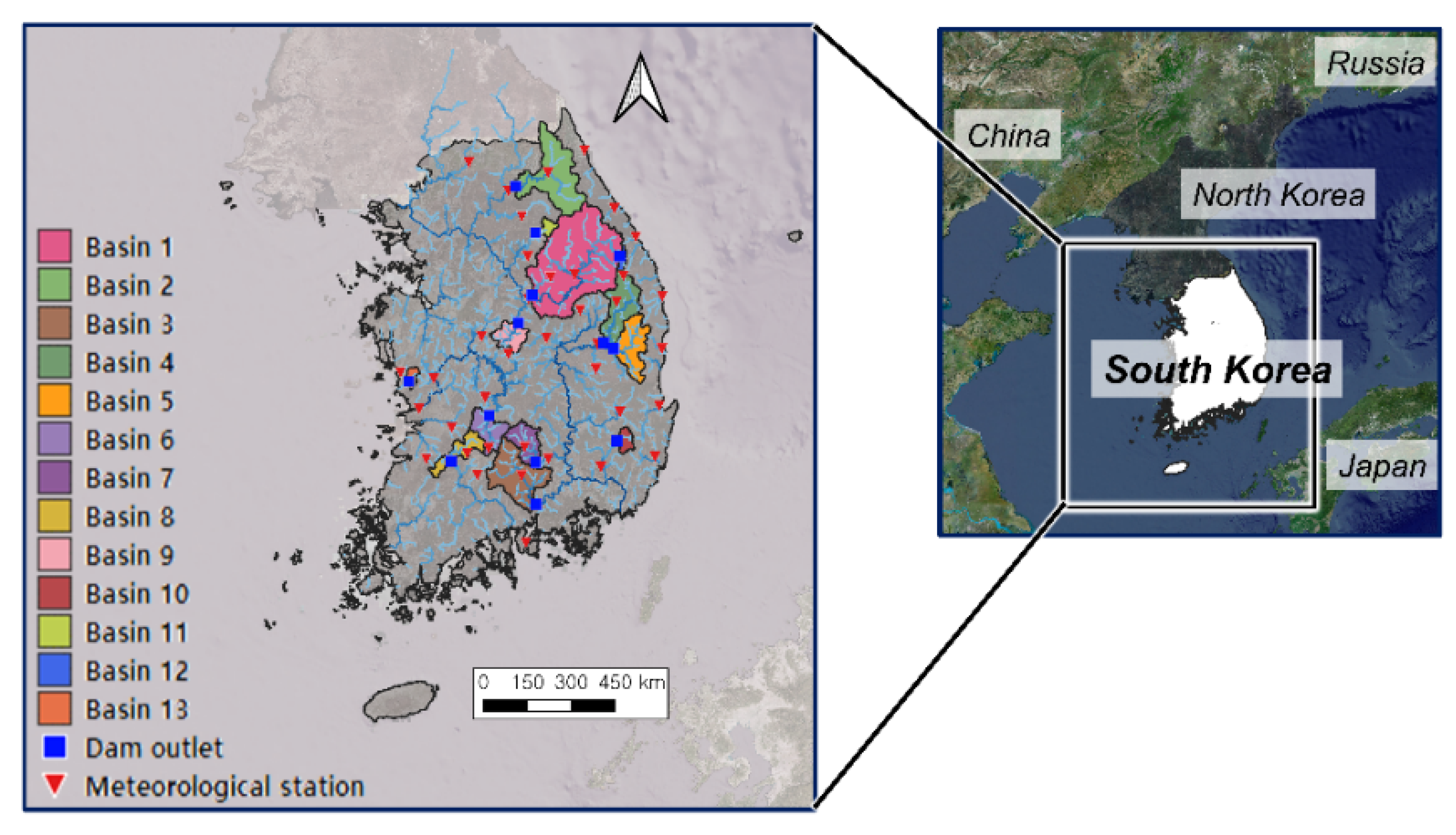
In this study, the performance of LSTM is evaluated for 13 dam basins in Korea, where streamflow data are available (see Figure 2). For the learning and prediction of LSTM, streamflow data and meteorological data from 2001 to 2020 were secured. We collected daily rainfall and other meteorological data—minimum and maximum surface air temperature, dew point temperature, and wind speed—that affect each study basin from the Meteorological Data Portal (data.kma.go.kr) of the Korea Meteorological Administration (KMA). Then, spatial mean time series for each basin were calculated using the Thiessen method. In addition, potential evapotranspiration for model input was calculated using the Penman-Monteith method from meteorological data [31,32]. Dam inflows observed at dams located at the end of each basin were considered the streamflow in the corresponding basin. Brief information on the selected basins is presented in Table 1.

2.3. Experimental Setup

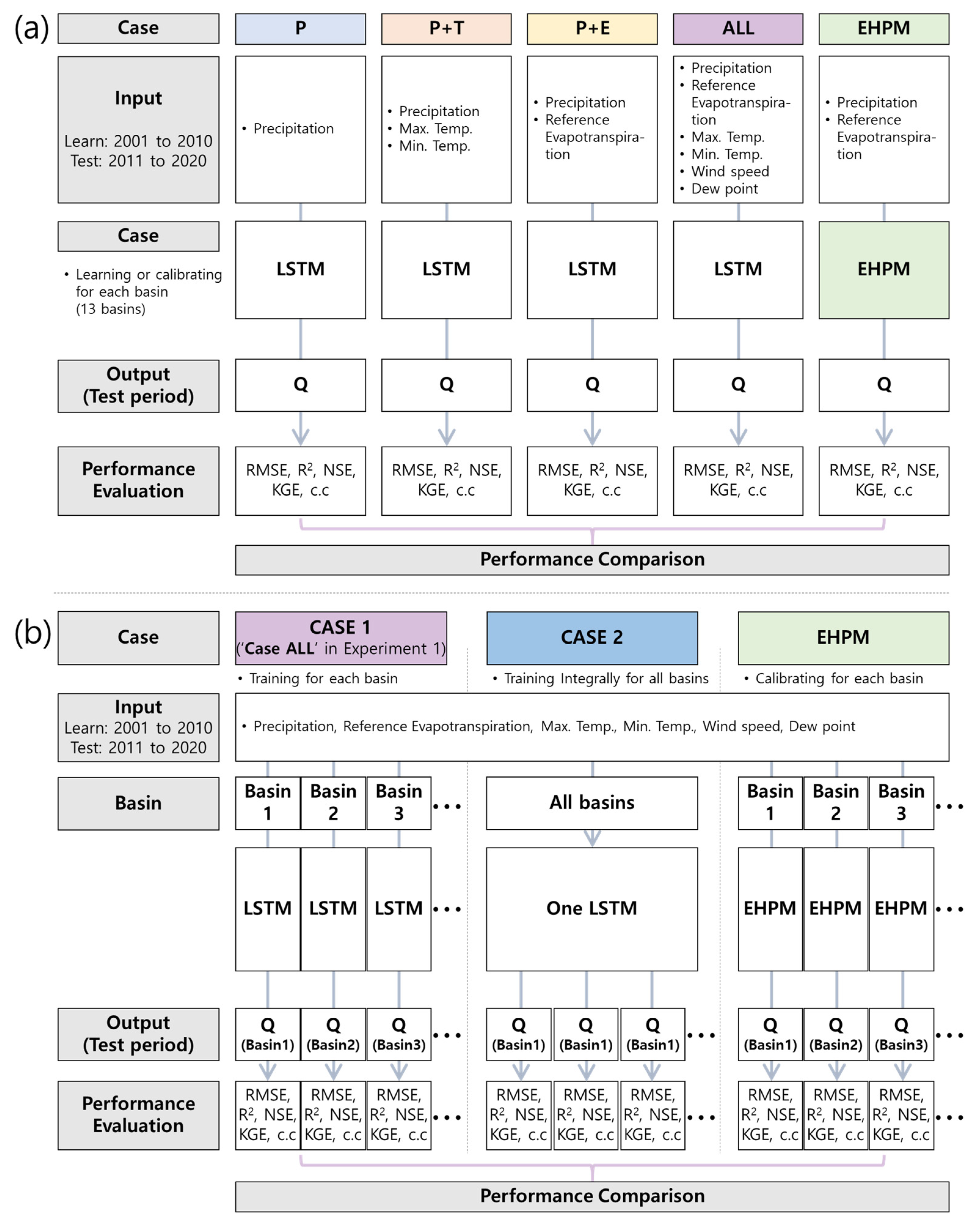
In this study, two experiments are performed, and Figure 3 shows the flowchart of each experiment. Section 2.3.1 and Section 2.3.2 describe each experiment in detail.

2.3.1. Experiment 1: Combination of Input Data for Learning

In the first experiment, our main question is how to construct the input data in hydrologic modeling with LSTM networks. This experiment is a pre-experiment of the second experiment, which tests the general functionality of the constructed LSTM network for rainfall-runoff modeling and examines the performance changes by the composition of meteorological data for learning.
As mentioned above, inputting rainfall is essential for learning LSTM for rainfall-runoff modeling, and temperature information is used additionally in some cases (see Section 1). In some data-rich areas, all observed meteorological information is used for learning. In the conceptual hydrologic model used as a benchmark in this study, potential evapotranspiration, one of the critical information in the basin hydrologic process, is used as input data along with rainfall data [29].
Therefore, in this experiment, four combinations of input variables are constructed: (1) using only rainfall data (Case P); (2) using rainfall and temperature (minimum and maximum) data (Case P+T); (3) using rainfall and potential evapotranspiration data (Case P+E); and (4) using all meteorological data (rainfall, minimum and maximum temperature, dew point temperature, wind speed, and potential evapotranspiration) (Case ALL).
Experiment 1 yields 52 separately trained networks (one for each of the 13 basins for four cases). To compare the prediction performance by the combinations of input data, we compared the streamflow predicted by each individually learned network with the observed streamflow.

2.3.2. Experiment 2: Multi-Basins Integrated Learning

For all data-driven approaches, networks learn the entire hydrological processes purely from training data. Deep learning models perform well when extensive long-term data are available [24]. An abundant training data set helps the networks learn relationships between the input and output sequences with more general and abstract patterns.
Therefore, training integrally multiple available basins may help gain a more general understanding of rainfall-runoff processes. For example, there are two basins with similar behavior, and the first of the two basins does not have extreme rainfall events or extended drought periods during the learning periods while having these events during the test period. If the second basin experienced similar events in the training set, the LSTM could learn the response behavior to these extreme events and use this knowledge in the first basin.
Based on this assumption, the second experiment aims to analyze how well the network architecture can be generalized (or regionalized) for all basins within a particular region. We trained one network by combining available data from all basins assuming that the 13 dam basins selected in this study have similar hydrological characteristics.

2.4. Model Evaluation

The LSTM learning progresses using the meteorological and streamflow data from 2001 to 2010. The trained LSTM networks use the meteorological data from 2011 to 2020 as input data to compute the predicted streamflow, which is evaluated by comparing it with the observed streamflow. The five metrics are used for model evaluation in this study are: (1) Root-mean-square error (RMSE); (2) coefficient of determination (R2); (3) Nash-Sutcliffe efficiency (NSE) [33]; (4) Kling-Gupta efficiency (KGE) [9]; and (5) correlation coefficient (c.c). All metrics are reported for the test period. The threshold of R2 and NSE for good performance is between 0.5 and 0.65 [34]. Likewise, if KGE is higher than 0.6, the simulations can be considered a good description of the observations [35]. RMSE close to zero indicates a small error between the simulations and the observations. A strong correlation is assumed when c.c > 0.7 [36,37].
For reference, our LSTM requires 365 days of antecedent meteorological data as input data to compute one streamflow (see Section 2.1.1), so we cannot simulate the initial year (2011) of test periods. The benchmark model also excluded the initial year for the evaluation because the warm-up period is essential to minimize the influence of the initial conditions. The practical evaluation of both data-driven and process-based models is calculated except for the initial years. Therefore, the performance of the predicted streamflow from 2012 to 2020 is evaluated in this study.

3. Results and Discussion

3.1. Best Combination of Input Variables for LSTM Learning

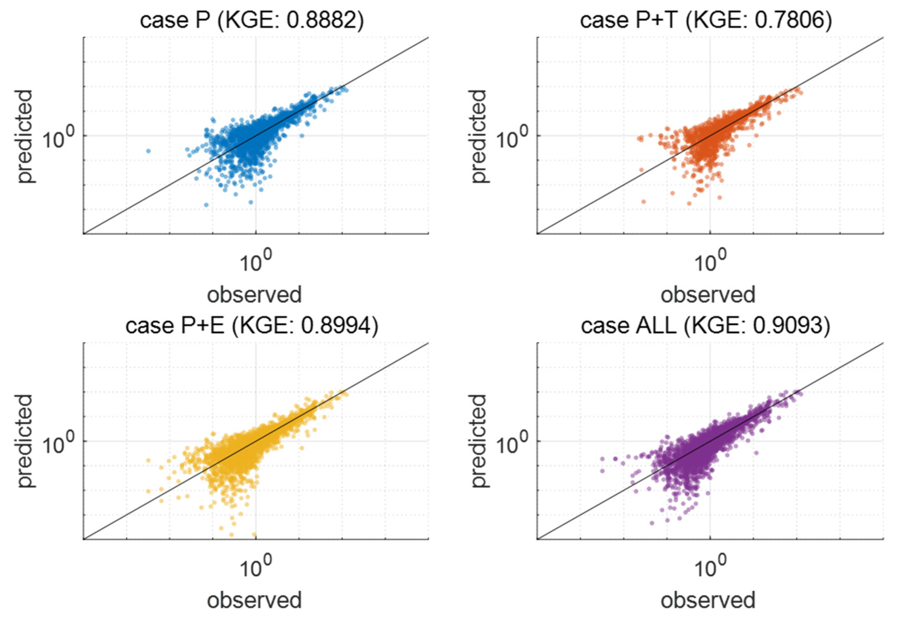
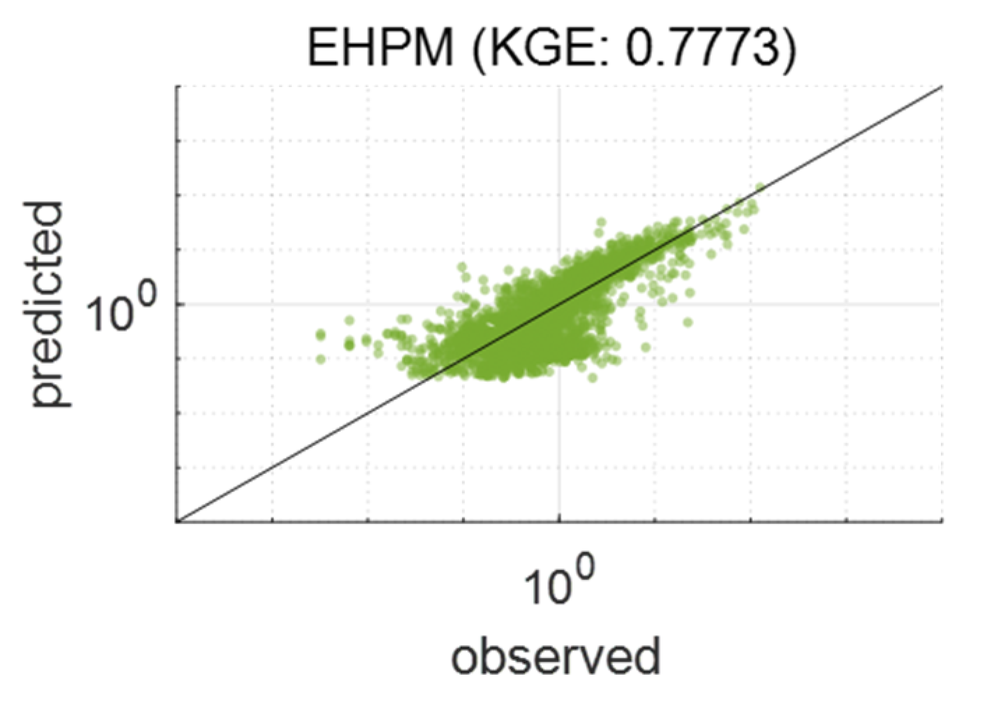
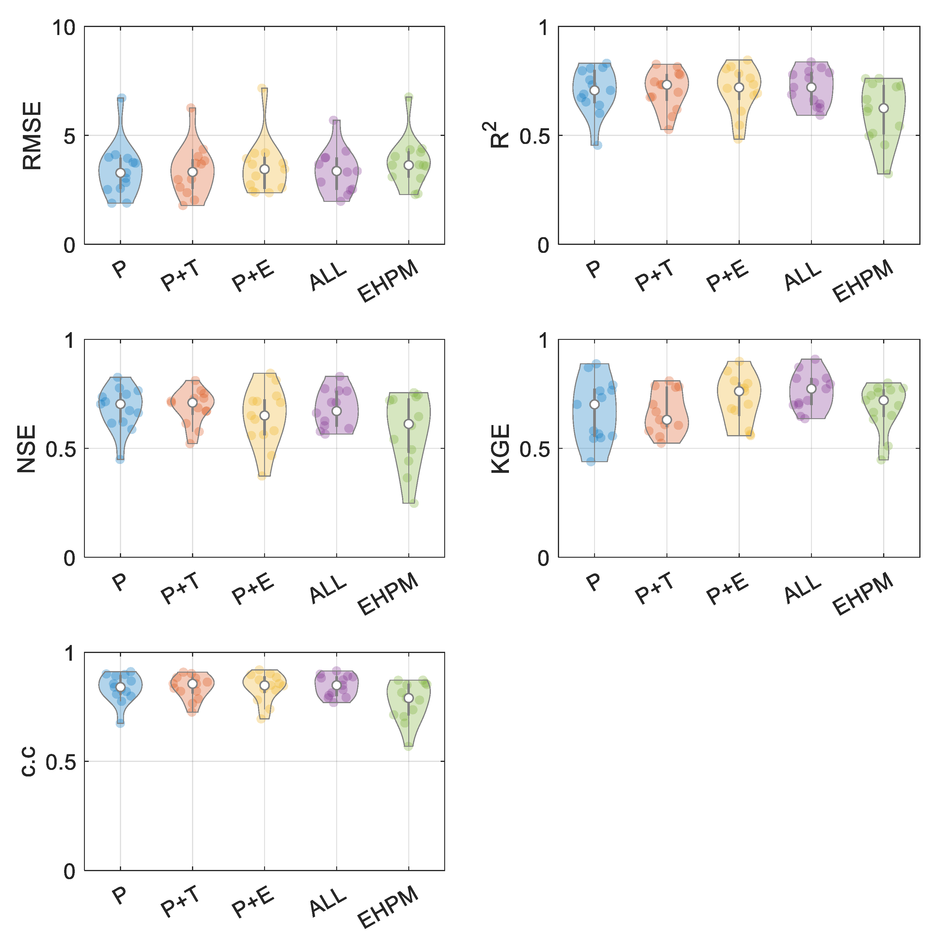
Figure 4 compares the predicted streamflow (2012–2020) in Basin 2 from each LSTM and EHPM as an example for Experiment 1, Figure 5 summarizes the performance of the models for all basins during the test period. The LSTM networks trained in this study show poor results in some applications, but all median values of each metric are above the thresholds, meaning that the trained LSTMs properly reflect the hydrological processes of each basin and predict the streamflow well overall.
The median values of RMSE, R2, and c.c for four applied cases are similar with about 3.28–3.43 mm/day, 0.71–0.73, and 0.84–0.86, respectively, but the performances between basins have some differences for cases. The LSTMs that learned only rainfall (case P in Figure 5) show the most considerable performance bias in most metrics, and the LSTMs that learned rainfall and potential evapotranspiration (case P+E in Figure 5) also show significant differences by basin. When learning rainfall and temperature (case P+T in Figure 5), it cannot be said that it is improved overall compared to case P, but the performance bias decreases compared to case P by adding temperature information.
In this result, we should notice that the LSTMs that learned all available meteorological information (Case ALL in Figure 5) perform relatively robustly. The NSE of this case shows a slightly lower median value than Cases P and P+T but the smallest bias. The KGE of Case ALL shows the highest median and slightest bias. Other metrics similarly show robust results regardless of the basin.
In learning the rainfall-runoff processes using only rainfall data as input, some applications show that it is relatively difficult to learn the abnormal hydrologic processes of a basin that are not explained by rainfall data alone. Errors in computing the potential evapotranspiration from meteorological data may be reflected in the learning of LSTM, which may degrade its performance. However, the results of Cases P+T and ALL show that the model can be made robust by adding the data. It means that the abnormal processes of a basin, which are challenging to learn only with rainfall information, can be learned relatively well by adding information such as temperature, dew point, and wind speed.
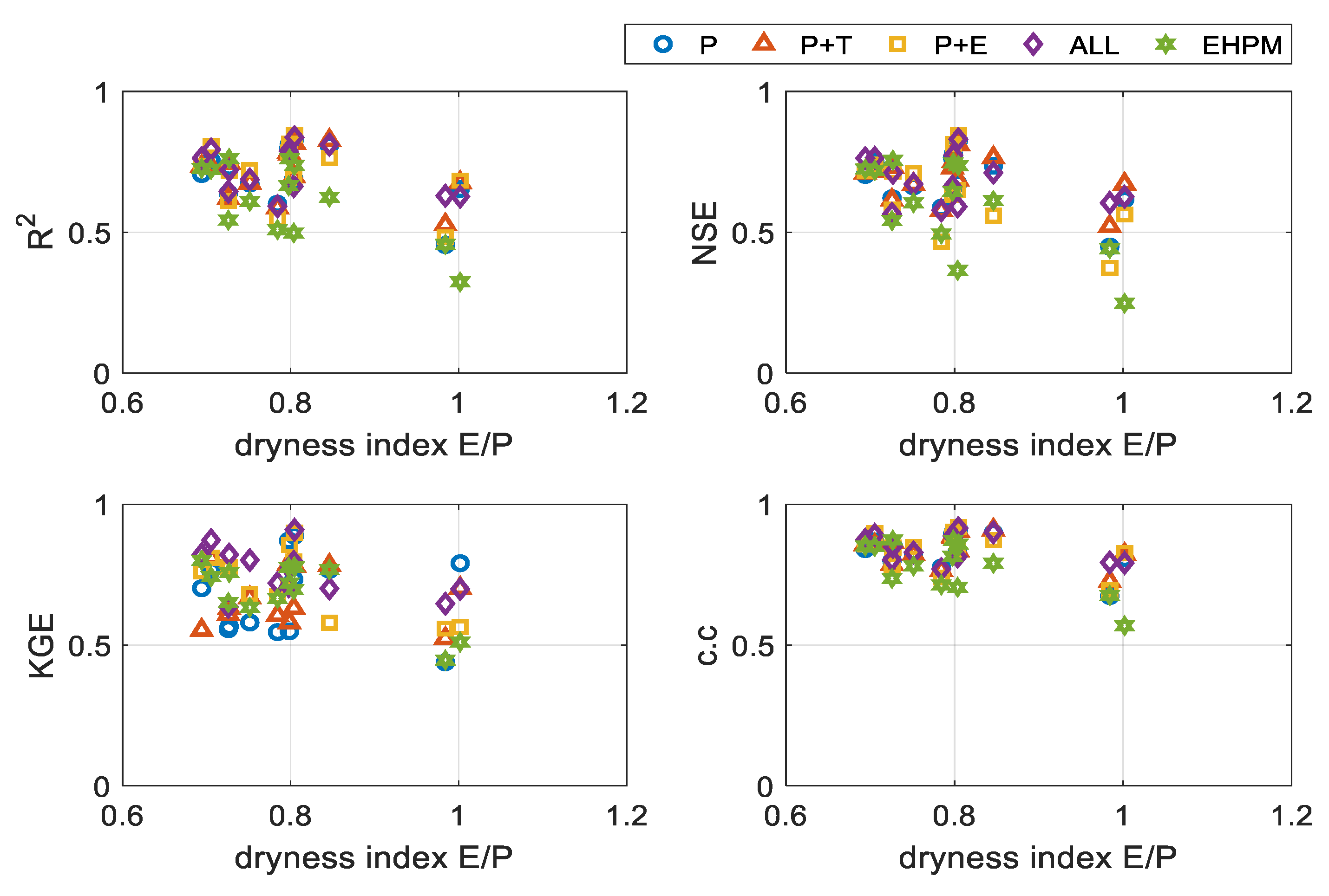
Furthermore, we calculated the dry index (annual potential evapotranspiration /annual rainfall) and then analyzed metrics for each case by considering it (see Figure 6). Here, RMSE, sensitive to the overall flow scale, was excluded from the analysis. As the dry index increases, the overall performance tends to decrease (although it is unclear in KGE). In particular, the benchmark model is more sensitive to dry conditions of the basins, which means that the process embedded in the model is difficult to reflect the hydrologic process in the dry basin.
The performance of LSTMs trained for four cases is also affected by the dry and wet conditions of the basins. LSTM primarily learns the rainfall-runoff process in a basin by learning the behavior of rainfall. However, drier basins have a higher proportion of processes in which rainfall is converted into infiltration and evaporation. It means the direct correlation between rainfall and runoff is bound to decrease, making learning the rainfall-runoff process difficult.
Nevertheless, Case ALL, which shows relatively robust performance with a slight bias between basins and a higher median value in Figure 5, are less affected by basin conditions. All additional meteorological input information is variables that can explain the hydro-meteorological conditions of the basins. For example, the surface temperature is closely related to soil moisture and vegetation growth, which is one of the variables that explain the infiltration and evapotranspiration processes. Dew point temperature, wind speed, and potential evapotranspiration can all help an LSTM learn hydrological processes that are difficult to learn from only rainfall. Our results suggest that using all available meteorological variables as input data in hydrological modeling using an LSTM may help output more robust results.

3.2. One LSTM for Predicting Streamflow in Each Basin

Since using all meteorological information as input variables showed the best results in Experiment 1, all information was likewise used as input data for LSTM in Experiment 2. In Experiment 2, the outputs from one model trained with data integrating information from all basins were analyzed.
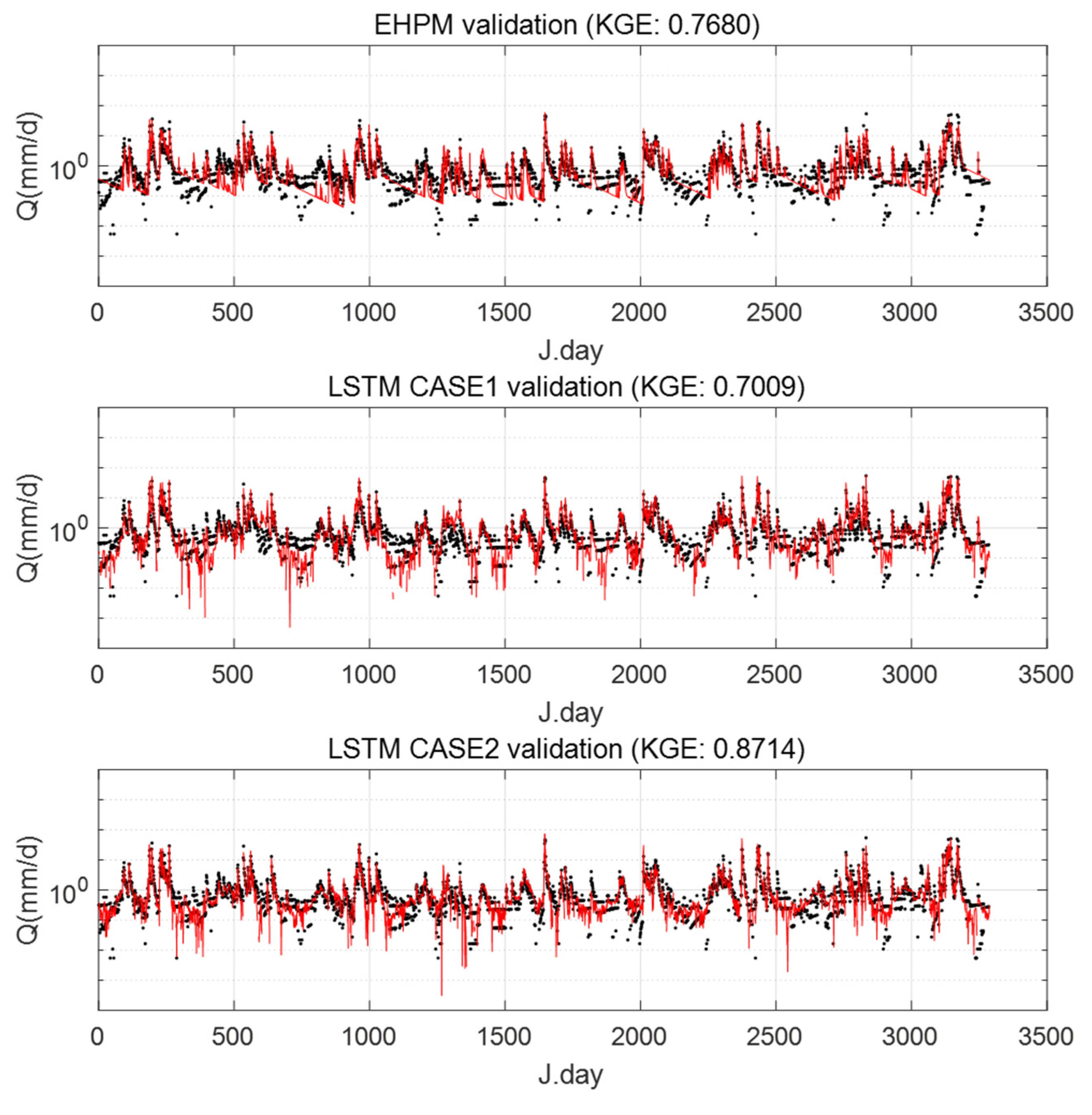
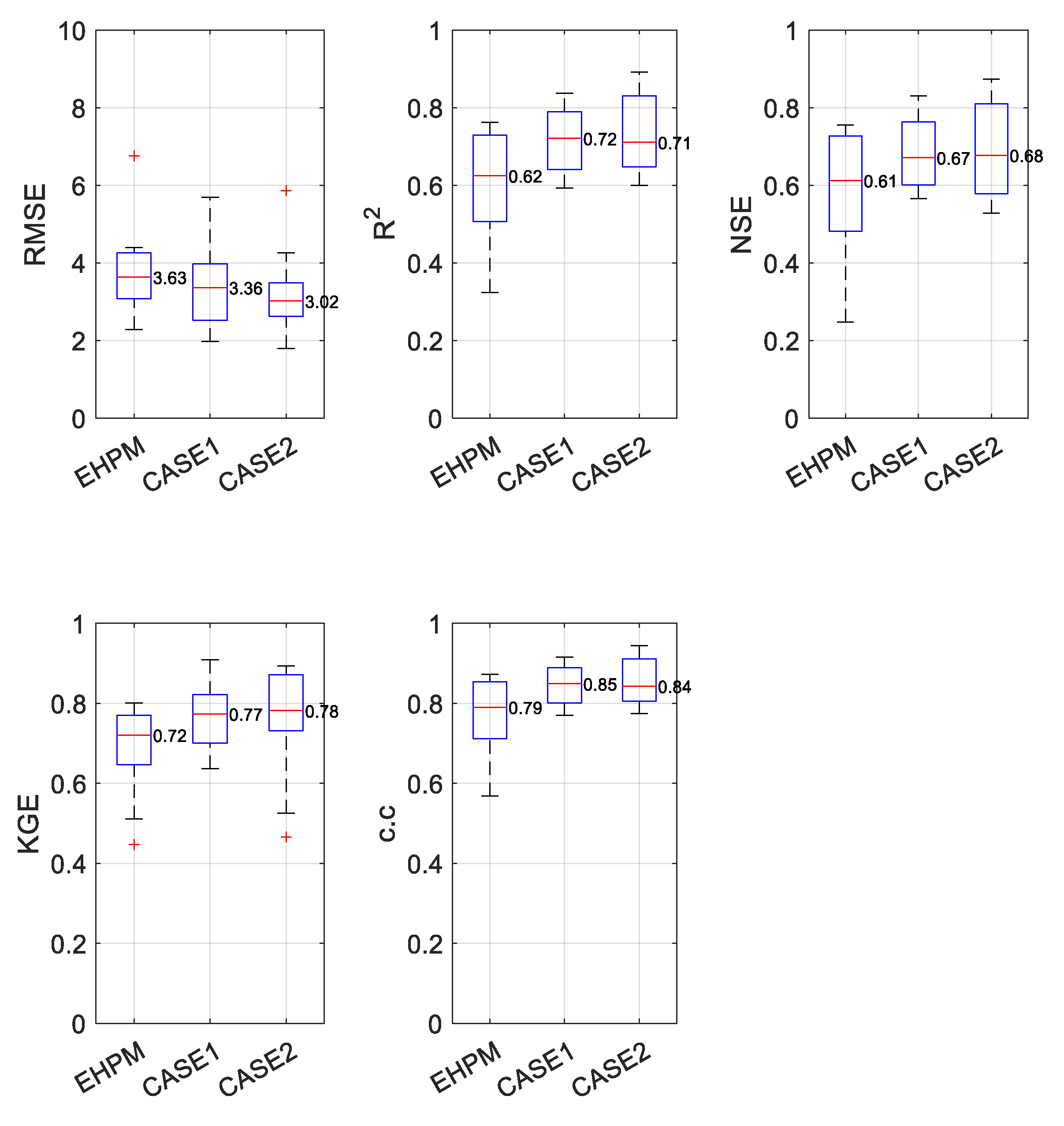
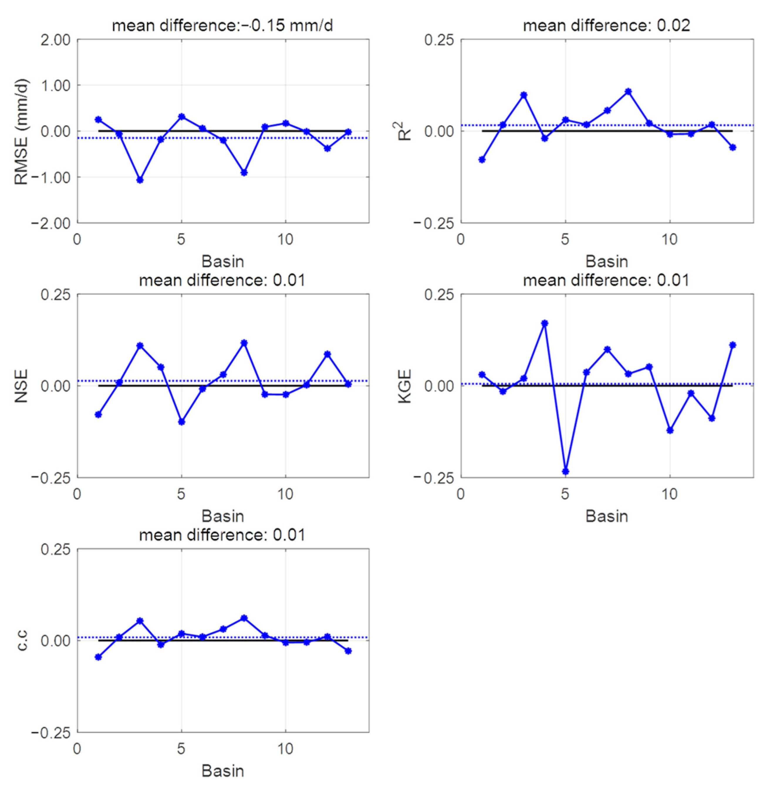
Figure 7 is an example (Basin 4) of the observed and predicted streamflow time series during test period for each case, and Figure 8 summarizes the performances for all basins as box plots. Here, CASE 1 shows the performances of 13 LSTMs learned separately using all meteorological data for each basin in Experiment 1 (i.e., case ALL in Figure 5), and CASE 2 shows the performance for each basin from one LSTM learned with all meteorological data for all basins. The median value of each metric for CASE 2 showed better performance than the benchmark model (see Figure 8). However, in all metrics, there are no significant differences from CASE 1. NSE and KGE increased by 0.01, while R2 and c.c decreased by 0.01. The median value of RMSE was improved by about 10%.
For a more detailed comparison, the differences (CASE 2 minus CASE 1) for each metric for each basin are shown in Figure 9. For some basins, the integrally learned model (CASE 2) is worse than the separately learned model (CASE 1). However, it can be confirmed that most performance is similar or improved except for Basin 5 in Figure 9, although it varies depending on a metric. The runoff ratio of Basin 5 is 0.42 (see Table 1), which is significantly different from the rest of the basins having a range of 0.50 to 0.68. We assumed that all study basins have similar hydro-meteorological characteristics, but Basin 5 actually has different characteristics. A low runoff ratio means the basin is relatively dominated by infiltration, storage, or evapotranspiration processes compared to other basins. To solve this problem, building a more generalized model by learning more basins or a more regionalized model by grouping basins with consideration for their characteristics is necessary. However, it seems that the integrally learned LSTM in this experiment is also generalized well enough to reasonably predict streamflow in the basins (see Figure 8 and Figure 9).
The main implication of the result of this experiment is that a model that reasonably performs in any basins within any region (i.e., a well-generalized model) can potentially be used as a tool for predicting streamflow in an ungauged basin. The streamflow prediction in ungauged basins is one of the significant challenges in the hydrology field [38,39]. However, much data is needed to account for the rainfall-runoff process and variations across various spatial and temporal scales, making streamflow simulation in the data-scarce region particularly difficult [40]. Similar to the integrated learning of this study, [41] has satisfactorily predicted ungauged basins that were not included in training by simultaneously learning several gauged basins. Our results of this experiment also show that the LSTM, which is integrally learned for information from all basins, is well generalized. Although no significant improvement was confirmed, this experiment shows that LSTM networks can be used to predict ungauged basins through further research.

3.3. Performance Evaluation for Flow Segments

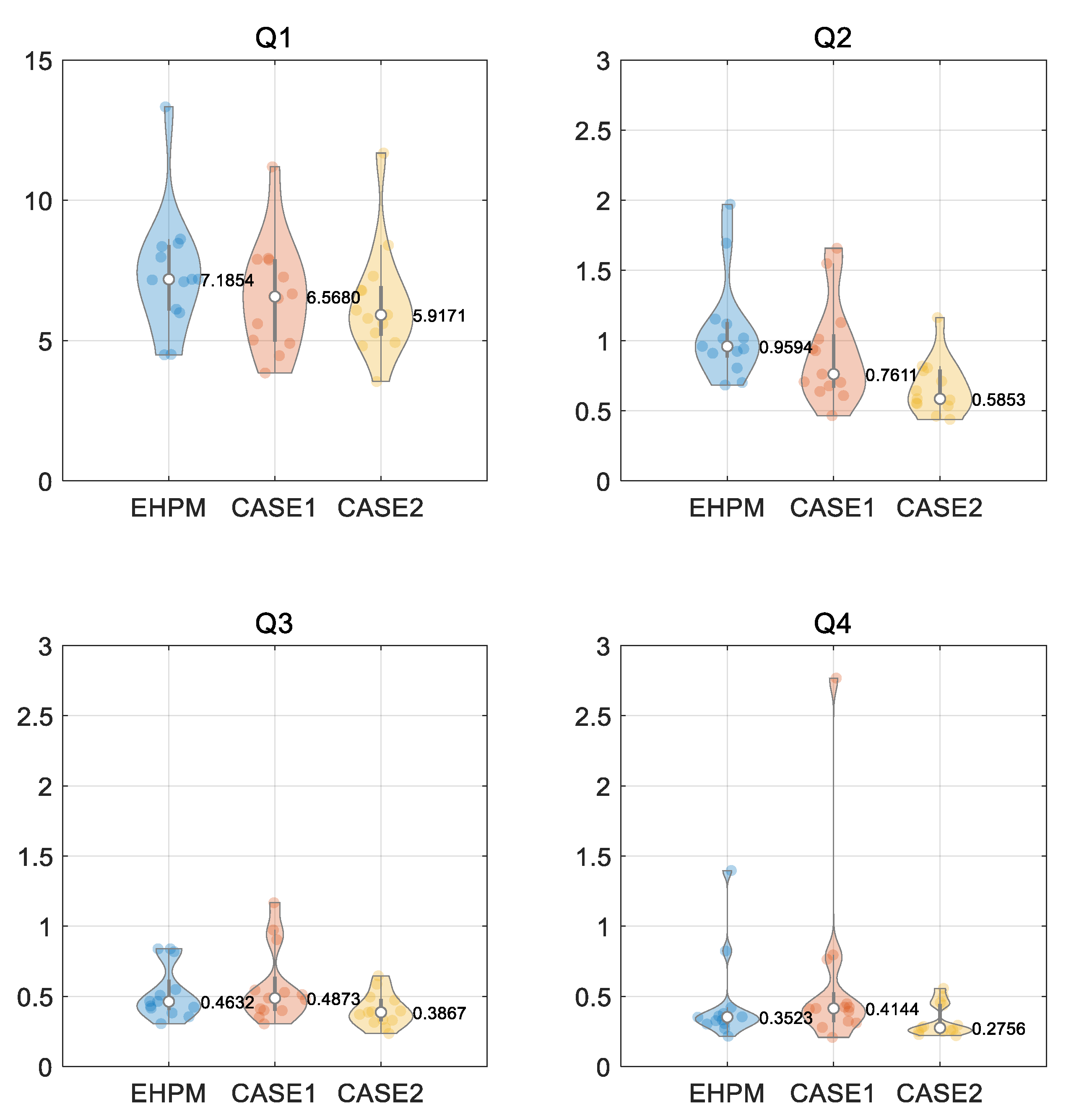
The integrated learning is one way to supplement insufficient learning data. If different rainfall-runoff processes can be learned in multiple basins, there is a possibility of learning the processes that cannot be learned in independent training. To reinforce the analysis in Section 3.2, we divided the observed streamflow into four segments at the same interval from top to bottom (see Table 2) and computed the RMSE of the predicted streamflow corresponding to the observations for each segment (see Figure 10). CASE 2 in Figure 10 shows that the RMSE decreases overall as information on multiple basins is learned. In particular, the RMSE of the low-flow segment (Q4) had a median value of 0.4144 with outliers when individually trained (CASE 1), but the median of the errors decreased by about 33% with the significantly reduced bias between watersheds through the integrated learning (CASE 2).
Monitoring daily hydrological situations and managing water resources require low flow predicting accuracy. Accurate prediction performance for low flow is essential for water resource planning to maintain a healthy watershed ecosystem [42]. In general, hydrologic models can simulate medium and high-flow reasonably well, yet accurate low-flow prediction remains a challenge [43]. The result shows that the integrated learning method can improve the accuracy of low-flow prediction and provide robust performance.
It is presumed that the LSTM, which has integrally learned the information for all available basins, has acquired a stable low-flow process that cannot be trained by individual learning for one basin. It means the multi-basin integrated learning shows strength at a period when the evapotranspiration process or baseflow process is essential. On the other hand, the improvement of high flow by the integrated learning is insignificant because basin characteristics such as catchment scale, hillslope, and curve number act relatively stronger on the surface runoff process, in which high flow due to large rainfall is significant [44]. Therefore, further research may consider integrated learning adding basin characteristics as learning data to improve the prediction performance of LSTM for high flow.

3.4. Integrated Learning Considering a Basin Characteristic

In Section 3.2, we confirmed that it is difficult to predict the streamflow in a basin with different characteristics from other basins included in the integrated learning. Furthermore, including the basin with different characteristics in the learning may degrade performance for prediction in other basins. Therefore, we divided the basins into two groups considering basin characteristics and briefly examined the performance of the LSTMs integrally learned for each group.
In this study, Curve Number (CN), one of the indexes representing the hydro-geomorphic characteristics of a basin, was used to distinguish the characteristics of the study basins. CN is a function of some major rainfall-runoff properties in a basin [45]. Since CN reflects several properties of a basin such as hydrologic soil type, land use, and antecedent moisture conditions and typically used to directly calculate excess runoff (and infiltration) [46], it can be effective in classifying the difference in the rainfall-runoff process between basins.
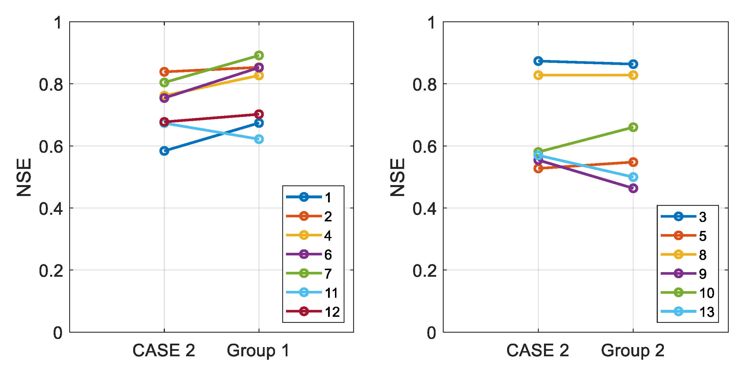
Based on the average CN of the basins, Group 1 consisted of 7 basins (Basins 1, 2, 4, 6, 7, 11, and 12) with lower CN values, and Group 2 consisted of 6 basins (Basins 3, 5, 8, 9, 10, and 13) with higher CN values (see Table 1). Data sets integrated for the basins in each group were individually used to learn two LSTMs. The performance of the two LSTMs was compared with CASE 2, the LSTM learned for all basins in Section 3.2, by predicting streamflow for the basins included in each group (see Figure 11).
The prediction performance in the case of learning only the basins with lower CN (Group 1) was improved in all basins except for Basin 11 than in the case of learning all basins (CASE 2). This result shows that grouping with proper consideration of basin characteristics can improve the performance of the integrally learned LSTM.
Conversely, in Group 2, which is integrated learning by selecting basins with higher CN, the performances of three basins (Basins 3, 9, and 13) were degraded. Basin 5 has a CN similar to other basins in the group, but as mentioned above, the runoff ratio is 0.42, much lower than other basins (see Table 1 and Section 3.2). As the number of basins used for integrated learning decreases, it is speculated that Basin 5, with different hydrological processes from other basins, has a more significant adverse effect on the generalization (or regionalization) of LSTM. In addition, the surface flow process by rainfall is dominant in basins with large CN values so that individual basin characteristics can act relatively stronger in the basins. Therefore, this result once again shows the need for further research on the appropriate grouping and composition of learning data.

4. Conclusions

Two experiments demonstrated that LSTM could simulate streamflow with competitive performance compared to the traditional hydrologic model (EHPM in this study). In the first experiment, the prediction performance of the LSTMs by each input variable combination was compared, and in the second experiment, one model was trained for all study basins and evaluated its performance.
This study aims to explore the method’s potential, not to implement the best possible performance of LSTM for each basin. Therefore, thorough hyperparameter tuning for each basin can provide better performance of LSTM. However, our LSTMs show better performance than the traditional hydrologic model, mostly with metrics above their threshold.
In summary, the major results of this study are the following.
  • The performance and robustness of the outputs from LSTM can be enhanced by using various meteorological information as an input variable of LSTM;
  • The LSTM could reasonably predict streamflow in the basins through the integrated learning method. This result means that the integrated learning method is a possible approach for reducing the data demand, and the concept of regionalization can be applied to LSTM. This regionalization approach may also help the streamflow in ungauged basins through further research;
  • In particular, at least in the basins selected in this study, low-flow predictions are improved through the integrated learning;
  • The selection of target basins for the integrated learning affects the performance of LSTM. Therefore, further research is needed on this topic.
The data-intensive nature of LSTM becomes a potential barrier in applications with data scarcity problems. Regionalizing an LSTM model through the integrated learning may be one of the ways to reduce the data demand of the model. However, more research is needed to promote the future application. For example, it is possible to investigate whether LSTM is improved by fine-tuning for a specific basin after integrated learning for multiple basins or evaluate the applicability of an LSTM, which is integrally learned, for ungauged basins. It is also necessary to examine the applicability of information generated from hydrologic models or data obtained through satellites as input data. In addition, it is necessary to examine in detail the low-flow prediction performance of the integrally learned model by specifying the drought periods.

Author Contributions

Conceptualization, J.C. and S.K.; methodology, J.C. and S.K.; validation, J.C., J.W. and S.J.; formal analysis, J.C. and J.W.; investigation, J.C. and J.W.; writing—original draft, J.C.; writing—review and editing, S.J. and S.K.; visualization, J.C. and J.W.; supervision, S.K.; project administration, S.K.; funding acquisition, S.K. All authors have read and agreed to the published version of the manuscript.

Funding

This research received no external funding.

Data Availability Statement

Data available on request.

Acknowledgments

This work was supported by a Research Grant of Pukyong National University (2021).

Conflicts of Interest

The authors declare no conflict of interest.

References

  1. Pagano, T.C.; Wood, A.W.; Ramos, M.H.; Cloke, H.L.; Pappenberger, F.; Clark, M.P.; Cranston, M.; Kavetski, D.; Mathevet, T.; Sorooshian, S.; et al. Challenges of operational river forecasting. J. Hydrometeorol. 2014, 15, 1692–1707. [Google Scholar] [CrossRef]
  2. Hirpa, F.A.; Salamon, P.; Alfieri, L.; Pozo, J.T.D.; Zsoter, E.; Pappenberger, F. The effect of reference climatology on global flood forecasting. J. Hydrometeorol. 2016, 17, 1131–1145. [Google Scholar] [CrossRef]
  3. Nourani, V. An emotional ANN (EANN) approach to modeling rainfall-runoff process. J. Hydrol. 2017, 544, 267–277. [Google Scholar] [CrossRef]
  4. Feng, D.; Fang, K.; Shen, C. Enhancing streamflow forecast and extracting insights using long-short term memory networks with data integration at continental scales. Water Resour. Res. 2020, 56, e2019WR026793. [Google Scholar] [CrossRef]
  5. Beven, K. Rainfall-Runoff Modelling: The Primer, 2nd ed.; John Wiley & Sons: Chichester, UK, 2001. [Google Scholar]
  6. Kratzert, F.; Klotz, D.; Brenner, C.; Schulz, K.; Herrnegger, M. Rainfall-runoff modelling using long short-term memory (LSTM) networks. Hydrol. Earth Syst. Sci. 2018, 22, 6005–6022. [Google Scholar] [CrossRef]
  7. Beven, K. Linking parameters across scales: Subgrid parameterizations and scale dependent hydrological models. Hydrol. Processes 1995, 9, 507–525. [Google Scholar] [CrossRef]
  8. Merz, R.; Blöschl, G.; Parajka, J.D. Regionalization methods in rainfall-runoff modelling using large catchment samples. IAHS Publ. 2006, 307, 117–125. [Google Scholar]
  9. Gupta, H.V.; Nearing, G.S. Debates--The future of hydrological sciences: A (common) path forward? Using models and data to learn: A systems theoretic perspective on the future of hydrological science. Water Resour. Res. 2014, 50, 5351–5359. [Google Scholar] [CrossRef]
  10. Xu, W.; Jiang, Y.; Zhang, X.; Li, Y.; Zhang, R.; Fu, G. Using long short-term memory networks for river flow prediction. Hydrol. Res. 2020, 51, 1358–1376. [Google Scholar] [CrossRef]
  11. Tanty, R.; Desmukh, T.S. Application of artificial neural network in hydrology-A review. Int. J. Eng. Technol. Res. 2015, 4, 184–188. [Google Scholar]
  12. Fang, K.; Shen, C.; Kifer, D.; Yang, X. Prolongation of SMAP to spatiotemporally seamless coverage of continental US using a deep learning neural network. Geophys. Res. Lett. 2017, 44, 11030–11039. [Google Scholar] [CrossRef]
  13. Shen, C. A transdisciplinary review of deep learning research and its relevance for water resources scientists. Water Resour. Res. 2018, 54, 8558–8593. [Google Scholar] [CrossRef]
  14. Shen, C.; Laloy, E.; Elshorbagy, A.; Albert, A.; Bales, J.; Chang, F.-J.; Ganguly, S.; Hsu, K.-L.; Kifer, D.; Fang, Z.; et al. HESS Opinions: Incubating deep-learning-powered hydrologic science advances as a community. Hydrol. Earth Syst. Sci. 2018, 22, 5639–5656. [Google Scholar] [CrossRef]
  15. Zhu, S.; Luo, X.; Yuan, X.; Xu, Z. An improved long short-term memory network for streamflow forecasting in the upper Yangtze River. Stoch. Environ. Res. Risk Assess. 2020, 34, 1313–1329. [Google Scholar] [CrossRef]
  16. Fang, K.; Shen, C. Near-real-time forecast of satellite-based soil moisture using long short-term memory with an adaptive data integration kernel. J. Hydrometeorol. 2020, 21, 399–413. [Google Scholar] [CrossRef]
  17. Hu, C.; Wu, Q.; Li, H.; Jian, S.; Li, N.; Lou, Z. Deep learning with a long short-term memory networks approach for rainfall-runoff simulation. Water 2018, 10, 1543. [Google Scholar] [CrossRef]
  18. Kratzert, F.; Klotz, D.; Shalev, G.; Klambauer, G.; Hochreiter, S.; Nearing, G. Benchmarking a catchment-aware long short-term memory network (LSTM) for large-scale hydrological modeling. Hydrol. Earth Syst. Sci. Discuss. 2019, 1–32. [Google Scholar] [CrossRef]
  19. Le, X.H.; Ho, H.V.; Lee, G.; Jung, S. Application of long short-term memory (LSTM) neural network for flood forecasting. Water 2019, 11, 1387. [Google Scholar] [CrossRef]
  20. Sudriani, Y.; Ridwansyah, I.; Rustini, H.A. Long short term memory (LSTM) recurrent neural network (RNN) for discharge level prediction and forecast in Cimandiri river, Indonesia. IOP Conf. Ser. Earth Environ. Sci. 2019, 229, 012037. [Google Scholar] [CrossRef]
  21. Sahoo, B.B.; Jha, R.; Singh, A.; Kumar, D. Long short-term memory (LSTM) recurrent neural network for low-flow hydrological time series forecasting. Acta Geophys. 2019, 67, 1471–1481. [Google Scholar] [CrossRef]
  22. Lu, D.; Konapala, G.; Painter, S.L.; Kao, S.C.; Gangrade, S. Streamflow simulation in data-scarce basins using Bayesian and physics-informed machine learning models. Journal of Hydrometeorology 2021, 22, 1421–1438. [Google Scholar] [CrossRef]
  23. LeCun, Y.; Bengio, Y.; Hinton, G. Deep learning. Nature 2015, 521, 436–444. [Google Scholar] [CrossRef] [PubMed]
  24. Schmidhuber, J. Deep learning in neural networks: An overview. Neural Netw. 2015, 61, 85–117. [Google Scholar] [CrossRef] [PubMed]
  25. Tian, Y.; Xu, Y.P.; Yang, Z.; Wang, G.; Zhu, Q. Integration of a parsimonious hydrological model with recurrent neural networks for improved streamflow forecasting. Water 2018, 10, 1655. [Google Scholar] [CrossRef]
  26. Hochreiter, S.; Schmidhuber, J. Long short-term memory. Neural Comput. 1997, 9, 1735–1780. [Google Scholar] [CrossRef] [PubMed]
  27. Ayzel, G.; Kurochkina, L.; Abramov, D.; Zhuravlev, S. Development of a Regional Gridded Runoff Dataset Using Long Short-Term Memory (LSTM) Networks. Hydrology 2021, 8, 6. [Google Scholar] [CrossRef]
  28. Bengio, Y.; Simard, P.; Frasconi, P. Learning long-term dependencies with gradient descent is difficult. IEEE Trans. Neural Netw. 1994, 5, 157–166. [Google Scholar] [CrossRef]
  29. Choi, J.; Kim, S. Conceptual eco-hydrological model reflecting the interaction of climate-soil-vegetation-groundwater table in humid regions. J. Korea Water Resour. Assoc. 2021, 54, 681–692. (In Korean) [Google Scholar]
  30. Vrugt, J.A.; Gupta, H.V.; Bouten, W.; Sorooshian, S. A Shuffled Complex Evolution Metropolis algorithm for optimization and uncertainty assessment of hydrologic model parameters. Water Resour. Res. 2003, 39, 1201. [Google Scholar] [CrossRef]
  31. Allen, R.G.; Pereira, L.S.; Raes, D.; Smith, M. Crop Evapotranspiration—Guidelines for Computing Crop Water Requirements—FAO Irrigation and Drainage Paper 56; FAO: Rome, Italiy, 1998; Volume 300, p. D05109. [Google Scholar]
  32. Won, J.; Choi, J.; Lee, O.; Kim, S. Copula-based Joint Drought Index using SPI and EDDI and its application to climate change. Sci. Total Environ. 2020, 744, 140701. [Google Scholar] [CrossRef]
  33. Nash, J.E.; Sutcliffe, J.V. River flow forecasting through conceptual models part I-A discussion of principles. J. Hydrol. 1970, 10, 282–290. [Google Scholar] [CrossRef]
  34. Ritter, A.; Munoz-Carpena, R. Performance evaluation of hydrological models: Statistical significance for reducing subjectivity in goodness-of-fit assessments. J. Hydrol. 2013, 480, 33–45. [Google Scholar] [CrossRef]
  35. Patil, S.D.; Stieglitz, M. Comparing spatial and temporal transferability of hydrological model parameters. J. Hydrol. 2015, 525, 409–417. [Google Scholar] [CrossRef] [Green Version]
  36. Safrit, M.J.; Wood, T.M. Introduction to Measurement in Physical Education and Exercise Science, 3rd ed.; Times Mirror/Mosby: St. Louis, MO, USA, 1995; p. 71. [Google Scholar]
  37. Ratner, B. The correlation coefficient: Its values range between+ 1/? 1, or do they? J. Target. Meas. Anal. Mark. 2009, 17, 139–142. [Google Scholar] [CrossRef]
  38. Sivapalan, M. Prediction in ungauged basins: A grand challenge for theoretical hydrology. Hydrol. Processes 2003, 17, 3163–3170. [Google Scholar] [CrossRef]
  39. Blöschl, G.; Sivapalan, M.; Wagener, T.; Savenije, H.; Viglione, A. Runoff Prediction in Ungauged Basins: Synthesis across Processes, Places and Scales; Cambridge University Press: Cambridge, UK, 2013; p. 465. [Google Scholar]
  40. Alipour, M.H.; Kibler, K.M. A framework for streamflow prediction in the world’s most severely data-limited regions: Test of applicability and performance in a poorly-gauged region of China. J. Hydrol. 2018, 557, 41–54. [Google Scholar] [CrossRef]
  41. Choi, J.; Lee, J.; Kim, S. Utilization of the Long Short-Term Memory network for predicting streamflow in ungauged basins in Korea. Ecol. Eng. 2022, 182, 106699. [Google Scholar] [CrossRef]
  42. Aryal, S.K.; Zhang, Y.; Chiew, F. Enhanced low flow prediction for water and environmental management. J. Hydrol. 2020, 584, 124658. [Google Scholar] [CrossRef]
  43. Nicolle, P.; Pushpalatha, R.; Perrin, C.; François, D.; Thiéry, D.; Mathevet, T.; Le Lay, M.; Besson, F.; Soubeyroux, J.-M.; Viel, C.; et al. Benchmarking hydrological models for low-flow simulation and forecasting on French catchments. Hydrol. Earth Syst. Sci. 2014, 18, 2829–2857. [Google Scholar] [CrossRef]
  44. Beven, K. Surface water hydrology-runoff generation and basin structure. Rev. Geophys. 1983, 21, 721–730. [Google Scholar] [CrossRef]
  45. Chatterjee, C.; Jha, R.; Lohani, A.K.; Kumar, R.; Singh, R. Estimation of SCS Curve Numbers for a Basin using rainfall-runoff Data. ISH J. Hydraul. Eng. 2002, 8, 40–49. [Google Scholar] [CrossRef]
  46. Bhuyan, M.J.; Borah, D.; Nath, B.K.; Deka, N.; Bora, A.K. Runoff Estimation of the Kolong River Basin in Assam, India Using NRCS-Curve Number Method and Geospatial Techniques. In Drainage Basin Dynamics; Springer: Cham, Switzerland, 2022; pp. 441–453. [Google Scholar]
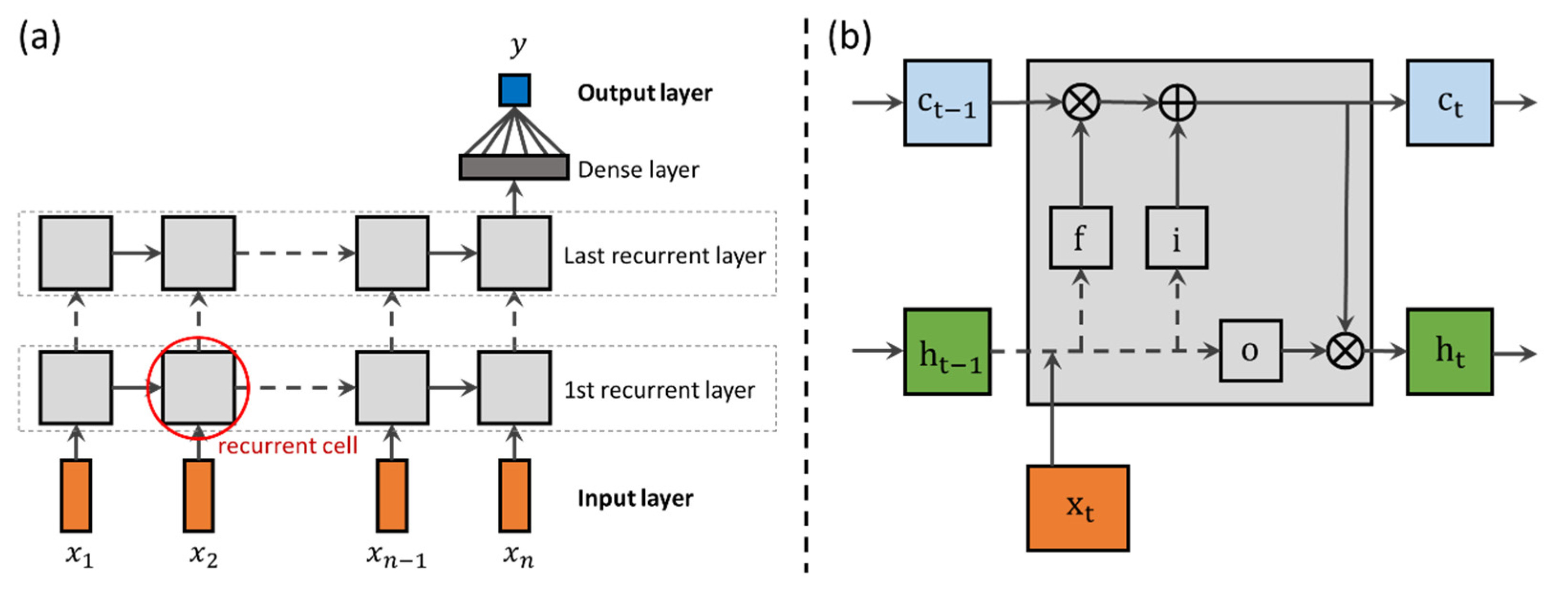
Figure 1. (a) Schematic diagram of a recurrent neural network. The input data (xt) for each time step (t) is input to each cell in the first recurrent layer, and the output of each recurrent cell is supplied to the cell of the next time step and the next recurrent layer. The output of the last recurrent layer in the last time step is supplied to the dense layer to calculate the final prediction (y); and (b) the internal operation of an LSTM cell, where f stands for the forget gate, i for the input gate, and o for the output gate. Note that xt denotes the input at time step t, ct denotes the cell state, and ht denotes the hidden state.
Water 14 02910 g001
Figure 2. Locations of study basins. Here, red markers on the map denote the location of meteorological stations, and blue markers denote the dams.
Water 14 02910 g002
Figure 3. Flowchart for: (a) experiment 1; and (b) experiment 2.
Water 14 02910 g003
Figure 4. Scatterplots of observed and predicted streamflow during the test period, where P is the case where only rainfall is input, P+T is where rainfall and temperature are input, P+E is where rainfall and potential evapotranspiration are input, ALL is where all meteorological information is input, and EHPM is the benchmark model.
Water 14 02910 g004aWater 14 02910 g004b
Figure 5. Summary of streamflow prediction performance during the test period (2012 to 2020). Here, P is the case where only rainfall is input, P+T is where rainfall and temperature are input, P+E is where rainfall and potential evapotranspiration are input, ALL is where all meteorological information is input, and EHPM is the benchmark model. Noted that circle markers are median values, and bars denote the first and third quartiles. Translucent dots are the results for each basin, and curved lines show the kernel density curves.
Water 14 02910 g005
Figure 6. Distribution of each performance metric for dry index.
Water 14 02910 g006
Figure 7. Observed and predicted streamflow time series in Basin 4 for each case. The black dots are the observed streamflow and red solid lines are the streamflow predicted by each case.
Water 14 02910 g007
Figure 8. Boxplots for streamflow prediction performances of the benchmark model (EHPM), the separately learned LSTM (CASE 1), and the integrally learned LSTM (CASE 2). Note that the red lines are median values, the blue boxes represent the first and third quartile, the whiskers represent the range between maximum and minimum values, and the red cross markers are the outlier. The value on the side of a box is its median value.
Water 14 02910 g008
Figure 9. Performance differences between the LSTMs separately learned for each basin (CASE 1) and the LSTM integrally learned for all basins (CASE 2). Note that solid black lines are zero-lines, solid blue lines represent the performance difference (CASE 2 minus CASE 1), and dotted blue lines represent the mean difference.
Water 14 02910 g009
Figure 10. Summary of RMSEs of streamflow predicted from each model for four flow segments. EHPM is the benchmark model, CASE 1 is the separately learned LSTM, and CASE 2 is the integrally learned LSTM. Note that Q1 is the segment for the top 0% to 25% flow magnitude, Q2 is for 25% to 50%, Q3 is for 50% to 75%, and Q4 is for 75% to 100%.
Water 14 02910 g010
Figure 11. Comparison of NSEs for the LSTMs integrally learned considering a basin characteristic (Groups 1 and 2) and the LSTM integrally learned for the entire basins in Section 3.2 (CASE 2). Here, Group 1 is a combination of basins with a relatively lower CN value, and Group 2 is a combination of basins with a relatively higher CN value.
Water 14 02910 g011
Table 1. Summary of hydro-meteorological information for the selected 13 basins.
Basin NumberBasin
Name
Area
(km2)
Annual Mean Precipitation, P
(mm/year)
Annual Mean Streamflow, Q
(mm/year)
Runoff
Ratio
Curve
Number
1Chungju6661.51305.7742.00.5764.2
2Soyanggang2694.31276.1803.50.6353.8
3Namgang2281.71519.81027.10.6865.2
4Andong1590.71178.0606.00.5161.4
5Imha1367.71115.5466.90.4267.8
6Yongdam930.41446.6815.90.5664.3
7Hapcheon928.91329.0712.50.5459.5
8Seomjingang763.51388.2785.60.5769.6
9Goesan676.71294.4651.10.5068.7
10Woonmoon301.91149.1705.50.6168.6
11Hoengseong207.91335.0777.70.5854.1
12Boryeong162.31160.5770.30.6659.1
13Gwangdong120.71311.2721.40.5570.1
Table 2. Classification of ranges for flow magnitude.
SegmentMagnitude of FlowRange of Percentile
Q1Highest flows0 to 0.25
Q2Higher flows0.25 to 0.5
Q3Lower flows0.5 to 0.75
Q4Lowest flows0.75 to 1
Publisher’s Note: MDPI stays neutral with regard to jurisdictional claims in published maps and institutional affiliations.