Article

Spatiotemporal Characteristics and Influencing Factors of Water Resources’ Green Utilization Efficiency in China: Based on the EBM Model with Undesirable Outputs and SDM Model

1
College of Urban and Environmental Sciences, Peking University, Beijing 100871, China
2
Institute of Spatial Planning and Regional Economy, Chinese Academy of Macroeconomic Research, Beijing 100038, China
3
Faculty of Architecture, Civil and Transportation Engineering, Beijing University of Technology, Beijing 100124, China
4
Guanghua School of Management, Peking University, Beijing 100871, China
5
Smart City College, Beijing Union University, Beijing 100101, China
6
Management College, Ocean University of China, Qingdao 266100, China
7
School of Environment, Beijing Normal University, Beijing 100875, China
*
Author to whom correspondence should be addressed.
Water 2022, 14(18), 2908; https://doi.org/10.3390/w14182908
Submission received: 11 August 2022 / Revised: 28 August 2022 / Accepted: 2 September 2022 / Published: 17 September 2022
(This article belongs to the Section Water Resources Management, Policy and Governance)

Abstract

:
A shortage of water resources is a global issue of common concern. The contribution of the article mainly includes the following two parts. First is the study of water resources’ green utilization efficiency (WRGUE) in 30 provincial administrative units of China from 2009 to 2019 by adopting the epsilon-based measure (EBM) model with undesirable outputs, which can yield a more accurate and reasonable assessment result. In addition, the spatial Durbin model was applied to analyze the driving factors of the WRGUE, which considers the spatial effects. The results are as follows: (1) The discrepancy of the WRGUE in different regions of China is conspicuous, with the highest in East China, followed by the central and the western region, while the Northeast is the lowest. A general decrease trend from China’s southeast coastal area to the northwest inland is presented. (2) Global spatial autocorrelation analysis shows a significant positive spatial autocorrelation in the WRGUE of the 30 sample provinces. However, the local spatial autocorrelation analysis shows that the WRGUE in China presents stronger spatial homogeneity than heterogeneity. (3) The levels of technology advancement, economic development, and the Opening-up policy implementation serve as positive factors influencing the WRGUE in China. On the contrary, the urbanization level has a significant negative impact on the WRGUE. The results of this paper may have great value for sustainable water resource utilization.

1. Introduction

Over the past 40 years since the reform and opening-up, China has made outstanding achievements in its economic growth, urbanization, and industrialization, which, however, have consumed vast quantities of water and caused severe environmental pollution [1]. According to the most recently released statistics by the National Bureau of Statistics of China (NBSC) [2], over the 17 years between 2004 and 2020, the discharge quantity of Chemical oxygen demand (COD) of wastewater has grown from 13.39 million tons to 25.65 million tons. Although China boasts rich water resources, its quantity per capita is rather limited [3,4]. If water resources are exploited without sound planning, the fact of water exhaustion will be exacerbated [5]. To tackle the water scarcity problem, one potential solution is to improve the utilization efficiency of water resource system [6]. Therefore, an in-depth discussion of the utilization efficiency of China’s water system is practical and of urgent need; it can provide a theoretical basis for future development strategies and policies for the optimal allocation of water resources.
At present, many scholars pay more attention to the water resource system efficiency. They mainly apply data envelopment analysis (DEA) [7,8,9,10,11,12,13,14,15,16] and stochastic frontier analysis (SFA) [15,16,17] to estimate the efficiency of water resource system, but these studies mainly have some defects. Firstly, the SFA method is a parameter estimation method that requires the evaluated parameters to be independent, but this requirement is very difficult to meet in reality [18,19]. Conventional DEA methods such as CCR, BCC, and SBM cannot take into account radial and non-radial characteristics simultaneously, which may lead to bias in the evaluation results [20,21,22,23,24,25]. Referring to the efficiency evaluation model, the paper adds water pollutant emission index to the evaluation systems and bring ups the concept of the water resources’ green utilization efficiency (WRGUE), which considers the unity of socioeconomic benefit and environmental benefit of water resources system, allowing for a more objective, accurate, and reasonable evaluation. Secondly, this paper is the first to use an epsilon-based measure (EBM) model with undesirable outputs to measure WRSGU in China, which has the following principal advantages: Considering both radial and non-radial characteristics at the same time when evaluating technical efficiency, considering undesirable outputs [26]. This evaluation method can yield a more accurate and reasonable assessment result.
The contributions of this paper lie in two aspects, as follows: (1) Measuring the WRGUEs of 30 provincial administrative units in China from 2009 to 2019 by means of an EBM model with undesirable outputs, thus revealing its sustainable utilization level. (2) Performing regression analysis of WSGUE by applying a spatial Dubin model (SDM) that takes the spatial autocorrelation into account, which can reveal the influencing factors of WSGUE more accurate, yielding government decision-making policy recommendations.
The body of the paper is organized as follows: Section 2 presents the methodology. Analogously, Section 3 introduces the data source and indicator selection. Results and discussions of WSGUE in China are in Section 4. Finally, Section 5 contains the main conclusions, policy recommendations, and future research directions.

2. Data and Methods

2.1. Research Area

This study selected relevant data of 30 provincial administrative units in China between 2009 and 2019 (Tibet Hong Kong, Macau and Taiwan are not estimated due to data limitation), as research material, which were divided into the Eastern, Central, Western, and Northeastern regions according to their socioeconomic development levels and geographical locations designated by NBSC (Figure 1). The Eastern and the Northeastern regions have abundant water resources due to the large rainfall amounts. By contrast, the inland provinces in the Western region, where water vapor is scarce, have little precipitation owing to the topography. On top of that, water resources in coastal areas are more abundant than in inland areas.

2.2. Index Selection and Data Sources

WSGUE Assessment Indicators

The required indicators were divided into three categories: the input indicators, the desirable output indicator, and the undesirable output indicators (Table 1). The specific categories are as follows:
(1)
Input indicators. We selected the total water consumption, employee index, and capital stock as input indicators. The total water consumption, including agricultural, industrial, domestic, and ecological water, referred to the data from NBSC [2]. The employee data came from the statistical yearbook of the Chinese provinces (2010–2020) [27].
(2)
The capital stock was estimated through the perpetual inventory method in this paper. According to Zhang et al. [28], the depreciation rate registered at 9.6%, and the capital stock in 2009 was equal to the investment in fixed assets divided by 10%. The price indices of the investment in fixed assets were converted to 2009 prices based in accordance with China Fixed Capital Investment Yearbook (2010–2013, 2015–2018) [29], China Investment Statistical Bulletin (2014) [30], China Investment Statistical Yearbook (2019–2020) [31], and NBSC [2].
(3)
The desirable output indicator. Gross regional product (GDP) was selected as the desirable output indicator in this paper. The provincial GDP was converted to 2009 prices based on GDP deflator. Relevant data were obtained from NBSC [2].
(4)
The undesirable output indicators. COD and nitrogen emissions from wastewater were selected, which have been the key monitored objects by the related department of environmental management in China for a long time, which are selected as two undesirable output indicators.

2.3. Driving Factors of WRGUE

The WRGUE is affected by many factors. On the basis of referring to previous studies, this paper selected the economic development level [4,32,33,34], water resources utilization structure [35], technical progress level [9,34,36], opening-up level [9,33,34], urbanization level [9,33,34], and population density [4,32] as the variables that affects the WRGUE. The data of this study was got mainly from NBSC [2]. The definitions of each variable are shown in Table 2.

2.3.1. Economic Development Level

In general, the higher the level of regional economic development, the higher the level of industrial agglomeration, production management, and technology. More resources can be applied to green technology innovation and water environment pollution control [36], which is good for WRGUE. Based on previous studies by Li et al. [4], Bao and Chen [32], Zheng et al. [33], and Zhang et al. [34], the economic development level was added to the regression model in this research.

2.3.2. Water Resources Utilization Structure

Agriculture is the key sector for water consumption and environmental protection. It was noted that agricultural water consisted of 70% of total water consumption, 62.1% of total COD discharged, 25.8% of total Ammonia Nitrogen discharged, and 7.3% of the country’s GDP in 2021 [2]. Therefore, agricultural water is the selected as the importance variables [35].

2.3.3. Technical Progress

Technological progress is the motive force of the upgrading of industrial structure, reducing the water input and increasing the output, and reducing water pollution emissions per unit of waste [36]. Therefore, we should assume that technical progress level has a positive effect on WRGUE. Learning from the previous studies by Zhou and Tong [9] and Zhang et al. [34], the motorization level was added to the regression model in this research.

2.3.4. Opening-Up Policy

Further implementation of China’s opening-up policy will speed up the spread and transfer of new technologies, boost products’ popularity, and reduce the water supply cost of production and living, thus alleviating the tension between the supply and the demand of water resources. According to Zhou and Tong [9], Zheng et al. [33], and Zhang et al. [34], the implementation level of the opening-up policy was selected as an important dependent variable.

2.3.5. Urbanization

The rapid urbanization in China can bring in a lot of agglomeration effects, such as communication cost reduction, the application of advanced technologies, etc. However, the development of urbanization in the short term may risk increasing the pressure on water resources [4], leading to the devastating result of water pollution. Overall, this paper selected the opening-up level as the important dependent variable [9,33,34], while the relationship between urbanization and WRGUE needs further empirical testing.

2.3.6. Population Density

Population density represents the degree of population concentration in urban. Generally speaking, the pressure on water resources in areas with high population densities will be considerable. Nonetheless, from another perspective, population growth can also bring agglomeration effects. Consulting the previous research of Li et al. [4] and Bao and Chen [32], this paper selected population density as an important variable for regression analysis.

2.4. Methods

2.4.1. The EBM Model with Undesirable Outputs

Data envelopment analysis (DEA) was first put forward by Charnes, Cooper, and Rhodes in 1978 [37]. Therefore, the original DEA model also was called the Charnes–Cooper–Rhodes (CCR) model. It has two advantages: It does not need to build up a function on the frontier and can deal with multi-input and multi-output efficiency assessment. In order to achieve the separation of technical and scale efficiencies, Banker, Charnes, and Cooper [38] achieved improvements to the CCR model that the separation of technical and scale efficiencies, so it is regarded as Banker–Charnes–Cooper (BCC) model. However, the inputs and outputs were assumed to proportionally increase or decrease when both of them were applied to calculating the technical efficiency, and therefore could not consider the slacks and were basically radial DEA model. Subsequently, Tone [39] proposed the slacks-based measure (SBM), which aims at obtaining maximum rates of reduction in inputs, relaxing the proportionality, and allowing independent changes to associated slacks when calculating the technical efficiency [40,41,42], but it neglects the radial factors and belongs to a non-radial DEA model. To resolve the shortcomings of radial and non-radial DEA models, in 2010, Tone and Tsutsui [20] proposed the epsilon-based measure (EBM) to combine both radial and non-radial factors. However, standard EBM model can neither consider undesirable outputs nor further compare multiple DUMs on the efficiency frontier simultaneously. To solve this problem, this paper applies the EBM model with undesirable outputs to calculate WSGUE, which has three advantages: Firstly, combining both radial and non-radial factors; secondly, considering undesirable outputs. The EBM DEA model with undesirable outputs can be represented as follows [26]:
θ = min ( κ ε x i = 1 m ω i b s i b x ro β + ε y r = 1 s ω r g s r b y ro + ε b p = 1 q ω p b s p b b p k ) s . t { j = 1 n x i j λ j + s i b = κ x i o i = 1 , 2 , , m j = 1 n y r j λ j s r g = β y r o r = 1 , 2 , , s j = 1 q b p j λ j + s p b λ = β b p o p = 1 , 2 , , q λ j 0 , s i b 0 , s r g 0 , s p b 0
where θ , κ , and β are the technical efficiency of the EBM DEA model with undesirable outputs, the radial DEA model, and non-radial DEA model, respectively. The range of values of them is [0,1]; n, s, m, and q represent the number of DUMs, the outputs, the inputs, and the undesirable outputs, respectively. s r g and s p b are the slacks of desired output r and undesired output p, respectively. ω r g and ω p b denote the desired output weight and the undesired output weight, respectively. bpk is the pth undesirable output of the DUMk; parameters ε y and ε b can combine the radial and non-radial slack. λ represents the intensity vector.

2.4.2. Spatial Autocorrelation Analysis

All things are interconnected, and the closer the proximity, the stronger the link becomes for them [43]. To examine the existence of spatial autocorrelation of WSGUE in the sample regions, we applied the spatial autocorrelation analysis method in this study, which can describe the spatial relationship of the attributes. There are plenty of methods for analyzing spatial correlation, among which the global Moran’s I and local Moran’s I are commonly employed. The global Moran’s I identifies the spatial correlation of observed objects from a global perspective, which is represented in Formula (2):
G l o b a l M o r a n I = i = 1 N j = 1 N W i , j W R G U E i , t W R G U E ¯ t W R G U E j , t W R G U E ¯ t 1 N i = 1 N W R G U E i , t W R G U E ¯ t 2 i = 1 N j = 1 N W i , j
where i and j are province i and province j, respectively; n stands for the number of provinces researched; and the spatial weight matrix is represented by Wij. If province i is adjacent to province j, Wij = 1, otherwise Wij = 0. W R G U E ¯ t is the average value of the WRGUE in the year t. The value range of Gloval Moran’s I ranges from –1 to 1. If the value is larger than 0, it indicates that there is a positive spatial dependence for WRGUE, while the value less than 0 represents a negative spatial autocorrelation.
L o c a l M o r a n I = N W R G U E i , t W R G U E ¯ t j = 1 N W i , j W R G U E j , t W R G U E ¯ t i = 1 N W R G U E i , t W R G U E ¯ t 2
The Moran scatter plot (MSP) map and local indicators of spatial association (LISA) map are commonly used to represent the results of local Moran’s I. The MSP and LISA maps are divided into four quadrants. The first quadrant means that the high WRGUE value of province is surrounded by high value, which is the high–high (HH) agglomeration area. The second quadrant indicates that the low WRGUE value of the province is surrounded by high value, which is the low–high (L–H) agglomeration area. The third quadrant is the low-low (L–L) agglomeration area, indicating that the low WRGUE value of the province is surrounded by low value. The fourth quadrant is the high–low (H–L) agglomeration area, which implies that high WRGUE value of province is surrounded by low value.

2.4.3. Spatial Durbin Model

There are three main spatial measurement methods, which correspond with different settings of spatial interaction. The first model is the spatial Lag model (SLM), which considers the endogenous interaction effect and assumes that part of the dependent variables in an area is affected by the dependent variables of its adjacent area. The second model is the spatial error model (SEM), which reflects the interaction effect between error terms. The SEM assumes that part of the error term in an area is affected by the error term of its neighboring areas. The third model is the Spatial Durbin model (SDM), which reveals the exogenous interaction effect and indicates that if the dependent variable in an area is affected by the dependent variable and independent variables of the neighboring area, the interpretation force of the SDM will also be stronger than those of the SLM and SEM [44,45,46,47,48,49]. Therefore, this paper chose the SDM to analyze the affected factors of WSGUE. The basic equation of the SDM can be expressed as:
Y = ρWY + βX + θWX + ε
where Y and X is the dependent and dependent variables; W stands for the spatial matrix; ρ represents the spatial lag autoregressive coefficient; β indicates the estimated coefficient of the independent variable; WX stands for the spatial lag term of independent, δ represents the corresponding spatial coefficient; and ε denotes a random perturbation term.
Before the spatial econometric analysis, firstly, the LR test and Wald test were conducted to examine whether the SDM could be reduced to the SAR and SEM. As shown in Table 3, all statistics of the spatial lag and spatial error were significant at the 1% levels; thus, with reference to Elhorst [50], the SDM should be selected. Next, the Hausman test proved random effects were rejected (chi2(6) = 109.49 ***), showing that fixed effect models were appropriate specifications in this paper. The SDM with fixed effects is therefore specified as follows:
Where DEL, WSUS, TDL, OPL, UL, and PD express Economic development level, Water resource utilization structure, Technological advancement level, Opening-up level, Urbanization level, and Population density, respectively. To avoid the problem of multicollinearity among variables, a VIF test was needed. As shown in Table 4, all values of VIF are less than 6; therefore, the multicollinearity concern is eased.

3. Results

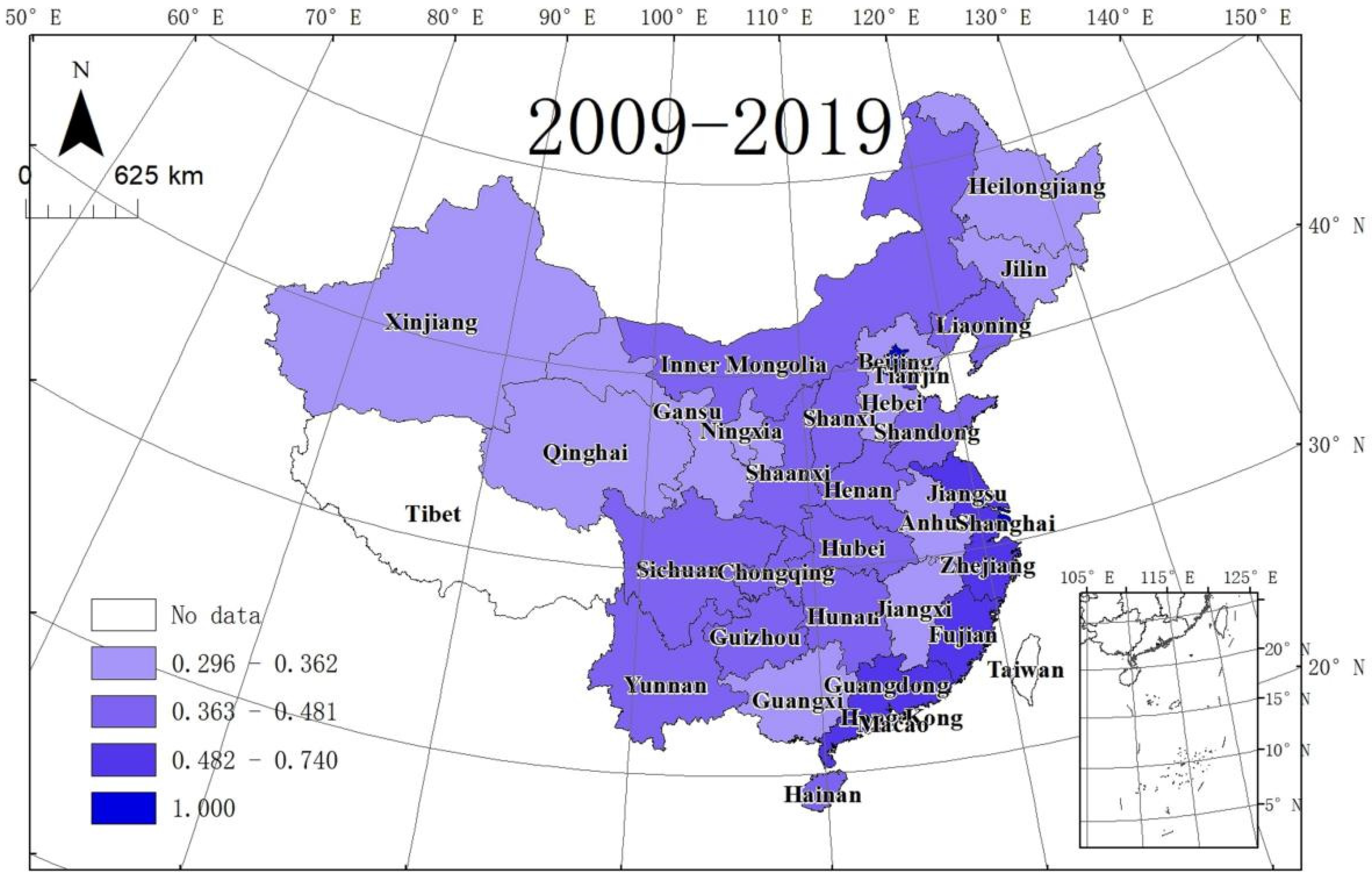
Based on the EBM model with undesirable outputs, the MaxDEA Ultra 8 software was used to evaluate the WRGUE values across the 30 provincial administrative units from 2009 to 2019. The specific calculation results are shown in Table 5. With the application of arcgis10.2 software, the spatial distribution map of the annual average WRGUE value during the studied years was made. As for Figure 2, the situation of WRGUE presents a general decrease trend from the southeast coastal area to the northwest inland. The WRGUE classifications were based on the Jenks Natural Breaks Classification Method [51]. The WRGUE was divided into four grades (from high to low).
Beijing and Shanghai are in the second class, and their WRGUE has reached the efficiency frontier during the studied years [52]. Beijing and Shanghai are two large cities and centers of technology in China. With the implementation of the policy to relieve Beijing’s non-essential functions as China’s capital and the upgrading of the secondary industry in Shanghai, many industries with high water consumption and pollution have moved to other regions, putting the WRGUEs of Beijing and Shanghai in the lead.
The second tier included Guangdong, Tianjin, Zhejiang, Jiangsu, and Fujian, and their values of the annual average WRGUE registered between 0.525 and 0.740. These provinces are mainly located in the eastern and southern coastal areas, where they maintain continued economic, technological, and management vitality. In recent years, with the upgrading of the industrial structure, the provinces have paid attention to environmental governance and rational utilization of resources; thus, the WRGUEs have been at a high level.
The third tier contained 13 provinces (Shandong, Chongqing, Hubei, Hunan, Henan, Inner Mongolia, Shaanxi, Shanxi, Liaoning, Hainan, Yunnan, Sichuan, and Guizhou), and their WRGUEs were located between 0.381 and 0.481. These provinces, enjoying relatively fast economic growth and urbanization, are mainly located in Central, Southwest, and North China, where water-saving technologies have reached a comparatively high degree of development and application.
The remaining ten provinces (Hebei, Anhui, Xinjiang, Heilongjiang, Gansu, Jiangxi, Guangxi, Qinghai, Ningxia, and Jilin) were in the fourth tier. Compared with the eastern provinces, the economic and technological development of these provinces is disappointing. To promote economic growth, many local governments in these provinces sacrifice water environmental protection by introducing water-consuming and energy-consuming industries, leading to heavy pollution; thus, they have a low level of WRGUE.

4. Discussions

4.1. Spatial Autocorrelation Analysis of WRGUE

The relationship between things is usually affected by the distance between them, and regional WRGUE belongs to regional variables according to the First Law of Geography. Therefore, before using the spatial panel measurement model to analyze the impact factors of WRGUE, the research should answer if the regional WRGUE has spatial autocorrelation. In this study, the spatial autocorrelation intensity of WRGUE of 30 provincial administrative units in China from 2009 to 2019 was analyzed by both the Global and Local Moran’s I index.
As observed in Table 6, all of the Global Moran’s I are positive, which passes corresponding significance level tests in the studied years. The figures show that WRGUE distribution has a strong spatial autocorrelation. The Global Moran’s I witnesses a fluctuating upward from 2009 to 2016, suggesting that the positive spatial autocorrelation of WRGUE is constantly strong. But the Global Moran’s I drops from 0.297 to 0.225 between 2016 and 2019, meaning that the positive spatial autocorrelation of WRGUE was weak.
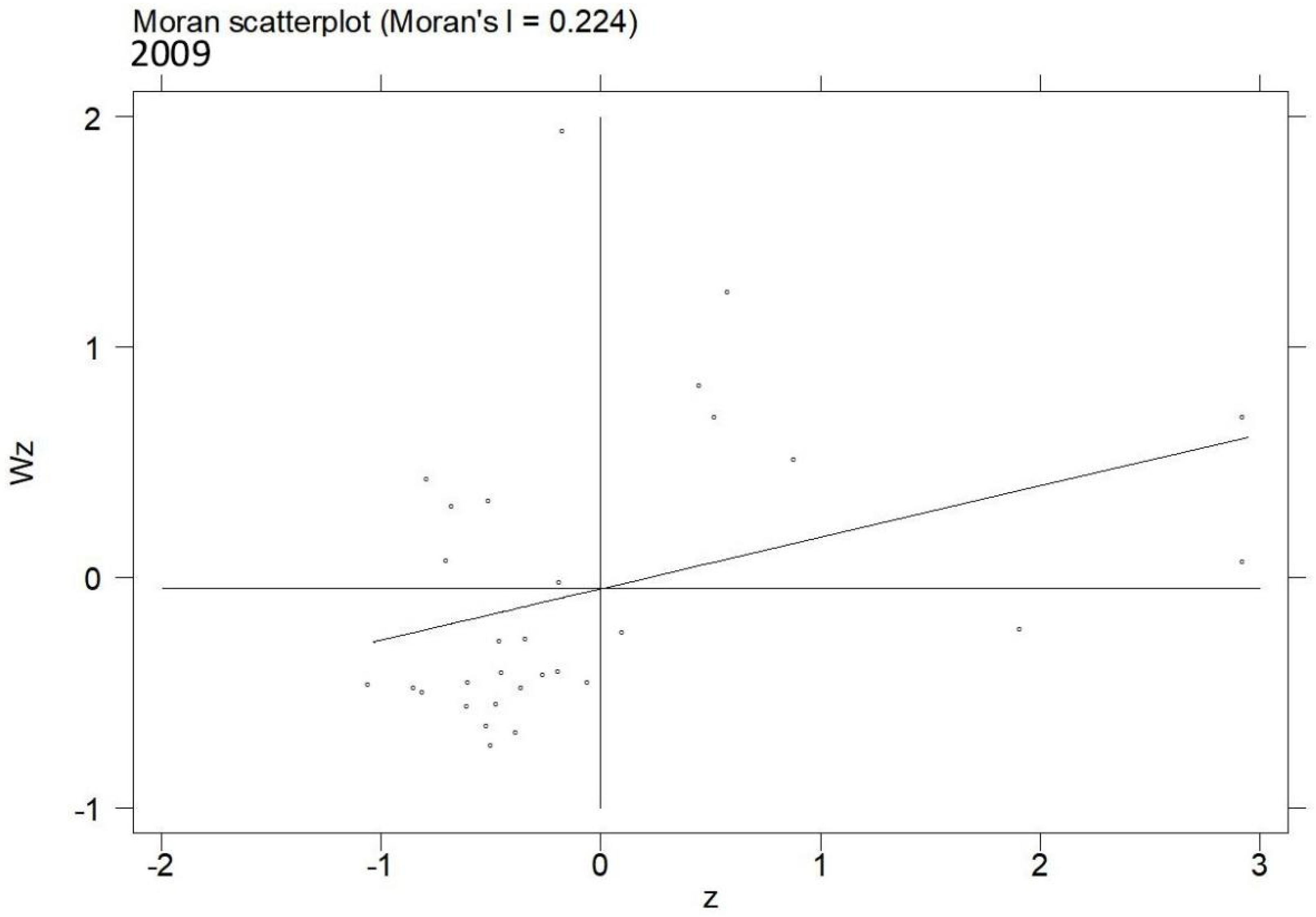
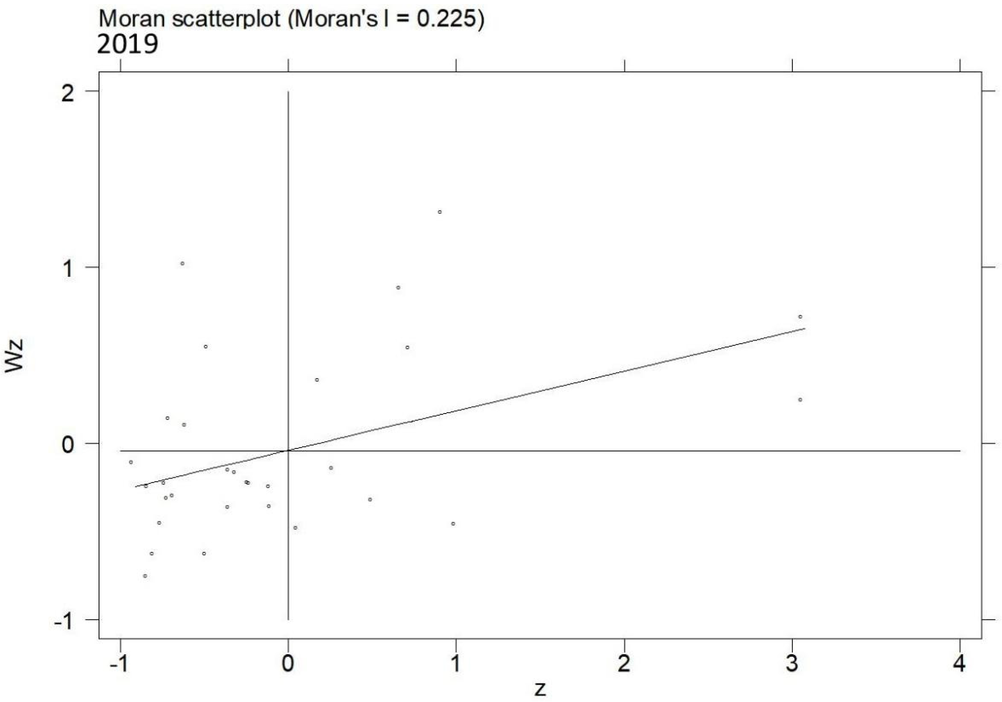
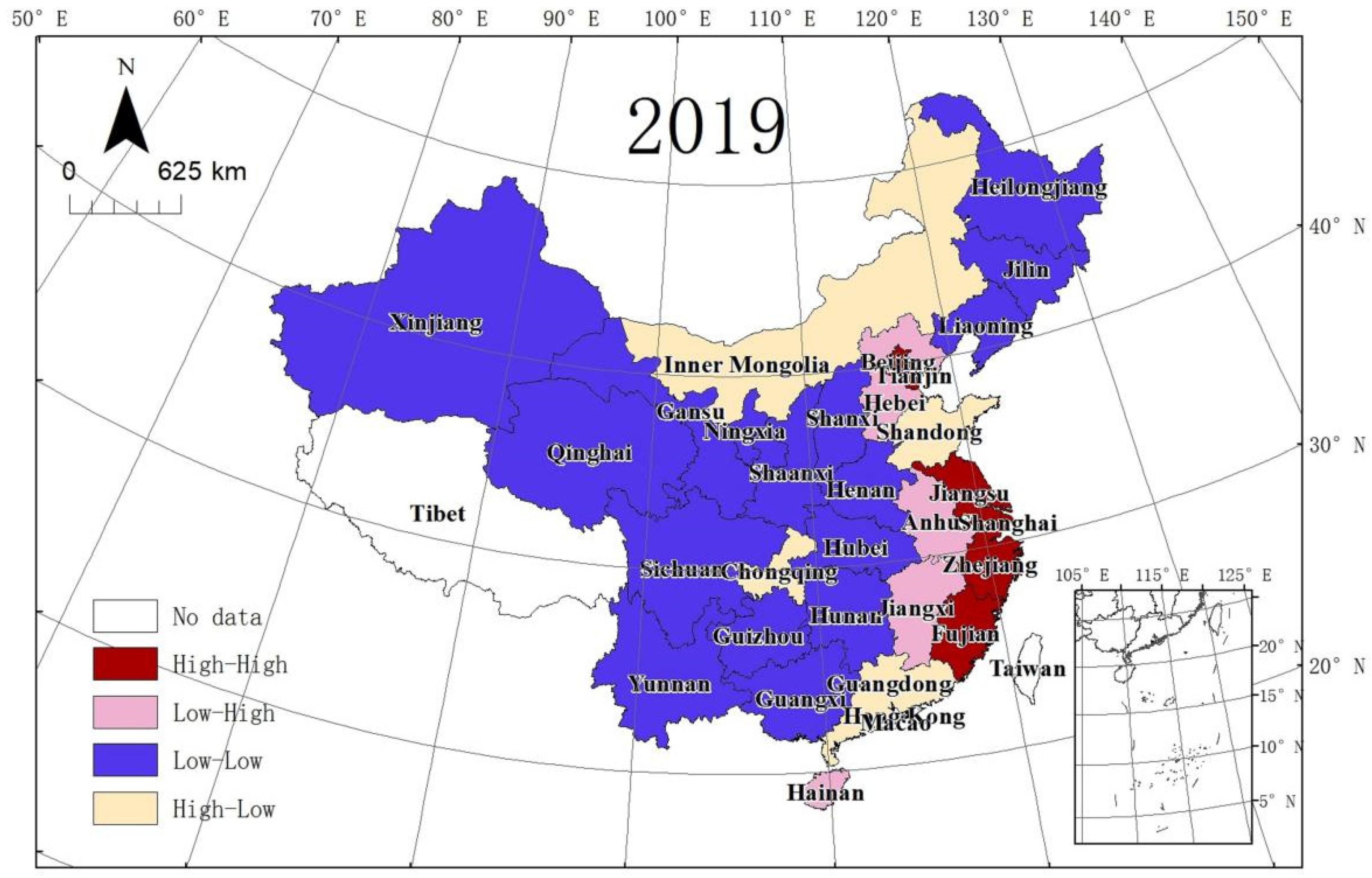
We used software Stata14 to calculate the local Moran’s I index of WRGUE in China based on Equation (4). Then, we drew the Moran scatter map between 2009 and 2019. In Figure 3 and Figure 4, the first quadrant comprises Beijing, Tianjin, Shanghai, Jiangsu, Zhejiang, and Fujian, all located in the eastern region, accounting for 20% of the total. The figures mean that major provinces in the eastern region have a higher level of WRGUE, showing a high degree of concentration. There are 17 provinces in the third quadrant, namely Shanxi, Inner Mongolia, Liaoning, Jilin, Heilongjiang, Anhui, Henan, Hubei, Chongqing, Sichuan, Guizhou, Yunnan, Shaanxi, Gansu, Qinghai, Ningxia, Xinjiang, accounting for almost 56.7% the total. The second quadrant contains Hebei, Jiangxi, Hunan, Guangxi, and Hainan, and the spatial characteristic of the WRGUE shows a low–high association. The fourth quadrant only includes Shandong and Guangdong, with a spatial characteristic of WRGUE showing a high–low association (their WRGUE levels are higher, but those of the surrounding provinces are lower).
Compared with the data in 2009, the first quadrant remains unchanged, while the third quadrant has lost two provinces (Inner Mongolia and Chongqing) and added one province (Guangxi), accounting for approximately 53.3%. The second quadrant has changed significantly by adding Anhui, covering Hebei, Jiangxi, and Hainan, and losing Hunan and Guangxi. As for the fourth quadrant, it has added Inner Mongolia and Chongqing, which were from the third quadrant (Figure 5 and Figure 6).
Overall, although the provinces in different quadrants have changed in recent years, more than 70% of the provinces have been in the first and the third quadrants, suggesting the WRGUE in China presents stronger spatial homogeneity than heterogeneity.

4.2. Discussion on Influencing Factors for of WRGUE

Table 7 displays the estimation results of spatial fixed-effects, time fixed-effects, and spatial and time fixed-effects. Based on the LR test, the assumption that spatial fixed effects are jointly insignificant is rejected (LR chi2(16) = 98.47 ***), and the assumption that the time fixed effects are jointly insignificant is also rejected (LR chi2(16) = 562.68 ***). From the value of Log-likelihood in Table 7, the spatial and time fixed-effects (521.8122) are more appropriate than the other two effects (472.5766 and 240.4700). Therefore, it is most reasonable to apply the SDM with spatial and time fixed-effects to empirical analysis.
The level of economic development and WRGUE show a positive relationship, which is in accord with the expectation. In 2019, the GDP per capita in China first broke the milestone of $10,000, which is over 66 times of the number in 1978 [2]. As Chinese economic development level rises, which provides a guarantee for the improvement of WRGUE. However, there is uneven development in various regions, which leads to the regional inequality of WRGUE to a certain extent. In the study period, the high level of WRGUE is mainly located in the eastern coastal region, which bursts with continued economic vitality in China. Due to the high level of opening-up, advanced technological progress and application, and effective management models, the WRGUE in the region registers high. In contrast, in regions with slow economic growth, such as Northwest China, it is necessary to continuously optimize the water resources’ utilization mode and draw the experience and technologies from eastern coastal regions.
It is found that water resource use structures have a minor influence on WRGUE, which is not evident. In recent years, the Chinese government has attached great importance to agricultural water conservation and formulated and promulgated the Outline of the National Agricultural Water Saving (2012–2020). The development and application of water-saving technologies in agriculture have been remarkable in China, which has offset the negative effects of the low efficiency of agricultural water. Technological advancement has positive correlations to WRGUE in a significant way, which is consistent with the expectation. With the economic growth remaining robust, China is ramping up its spending on research and development in many aspects. The R& D expenditure has increased from the 1.05% of the GDP in 2002 to 2.4% in 2021 [2]. These measures have provided a guarantee for the development of water-saving technologies in industry and agriculture. Hence, the reuse of industrial and agricultural wastewater has achieved great improvement in recent years.
The opening-up level serves as a significant positive factor to WRGUE, which agrees to expectation. Since joining World Trade Organization in 2001, China’s reform and opening drive has entered a new historic era. Currently, China has already become the largest trading nation in the world. China is the biggest trading partner for 163 countries in 2020. As China continues to deepen the reform and opening-up, many foreign advanced water use technologies have been introduced into China, which has strongly promoted WRGUE.
The level of urbanization has a remarkably negative effect on WRGUE, which indicates that rapid urbanization cannot bring the agglomeration effect of water resource utilization in China. Cities are the physical carrier for human beings to exist and live in, where a great amount of water is consumed. Recently, China’s urbanization rate has risen rapidly from 19.4% in 1978 to 60.6% in 2019 [2,53,54]. With the increase of urban population, the continuous growth of water demand, the severity of water pollution, and the shortage of water resources in some regions in China have become increasingly serious, restricting China’s sustainable development.
Population density has a not-so-significant negative relationship with WRGUE. The sewage discharge in areas with a dense population is commonly large. However, China has unremittingly given high priority to the education of water conservation and environmental protection in compulsory education; the idea of saving water resources has gained publicity in China in various ways. On the other hand, in recent years, with the level of economic development increasing, Chinese citizens’ expectations of the high-quality living environment are also increasing, and their water environmental protection awareness has increased. These background conditions may offset the negative impact of high population density to a certain extent.

5. Conclusions

Scientific and accurate evaluation of WRGUE is essential for promoting the sustainable water resources’ utilization and realizing the 2030 sustainable development goal of the United Nations [55]. This paper empirically examined the WRGUE in China, aiming to provide an objective assessment and support the sustainable utilization of water resources in China. The article first evaluated the WRGUE in 30 provincial administrative units of China using the EBM model with undesirable outputs, which found conspicuous regional differences of the WRGUE in different regions of China. Specifically, the efficiency is higher in the eastern region, followed by the central and the western region, while Northeast China is the lowest. The WRGUE presents a general decrease trend from the southeast coastal area to the northwest inland. Based on the spatial autocorrelation analysis, a significant positive spatial autocorrelation in the WRGUE of the 30 sample provinces is shown, and the WRGUE in China presents stronger spatial homogeneity than heterogeneity. In the end, the paper empirically analyzed the driving factors of WRGUE using the SDM method. It is found that the levels of economic development, technological advancement and opening-up are the significant positive influencing factors of the WRGUE in China. On the contrary, the level of urbanization has an obvious negative impact on the WRGUE.
Based on the results, this paper proposes some relevant policy recommendations: (1) Considering the existence of spatial effect of WRGUE, it is necessary to create more spillover channels to realize the coordinated development of regional WRGUE. High-efficiency provinces should enlarge communication and cooperation with low-efficiency provinces by sharing the advanced technology and administration methods. On the other hand, importing advanced water resource systems from other regions and getting rid of outdated and high water-consuming technologies are necessary for low-efficiency provinces. (2) Promoting technical innovation of the economic and infrastructure industries is critical to improve water resources usage efficiency. For instance, key industries such as mining and dyeing are required to transform and apply nitrogen processor and clean production procedures. In addition, more attention should be paid to industrial structure optimization, scientific and educational development, and transportation infrastructure enhancement. (3) The disparity in irrigational water use efficiency among areas should be made fully aware of. The government should attach greater importance to developing advanced agricultural technology and push forward effective water-saving and water conservation policies in low-efficiency regions. (4) Suitable water utilization regulations and a well-regulated water credits exchange market should be established. Meanwhile, market access and contamination restrictions should be imposed on the foreign-funded enterprises with the potential of high waste emission. (5) The government subsidies should be increased in water-saving projects, such as advancing water-recycling equipment, maximizing the utilization of rainwater, and building edge-cutting sewage treatment facilities.
With regard to the limitations of the study, there still exist many practical problems that deserve researchers’ attention and endeavor for further research. First, as the paper only focused on the WRGUE of administrative spaces, future work should focus on the WRGUE of specific industries and sectors, such as agriculture, mining, manufacturing, construction, power generation, transport, and so forth. Moreover, the ultimate goal of WRGUE research is to achieve the sustainable utilization of water resources. Therefore, further research should dive into the application and practice of an intelligent water resources system, which can maximize the use of water resources. Thirdly, there are obvious differences in the regional distribution of water resources in China; hence, it is of significant meaning in studying the regional balance of WRGUE. Therefore, further research should focus on the convergence of regional WRGUE in China, which can provide a theoretical basis for the regional balance and harmonious development of water resource utilization.

Author Contributions

L.Z.: Conceptualization, methodology, software, validation, formal analysis, writing—review and editing. P.L.: writing—review and editing. Z.Y.: funding acquisition, writing—original draft preparation, writing—review and editing. Y.N.: software, formal analysis. S.L.: writing—review and editing. G.G.: writing—review and editing. D.H.: writing—review and editing. All authors have read and agreed to the published version of the manuscript.

Funding

This research was funded by Carbon Neutralization Promotion Fund of China Green Carbon Foundation.

Institutional Review Board Statement

Not applicable.

Informed Consent Statement

Not applicable.

Data Availability Statement

The data were obtained from China Fixed Capital Investment Yearbook (2010–2013, 2015–2018), China Investment Statistical Bulletin (2014), China Investment Statistical Yearbook (2019–2020) and NBSC.

Conflicts of Interest

The authors declare no conflict of interest.

References

  1. Zhou, X.; Luo, R.; Yao, L.; Cao, S.; Wang, S.; Lev, B. Assessing integrated water use and wastewater treatment systems in China: A mixed network structure two-stage SBM DEA model. J. Clean. Prod. 2018, 185, 533–546. [Google Scholar] [CrossRef]
  2. National Bureau of Statistics of China. China Statistical Yearbooks (CSY) (2009–2018); China Statistical Publishing House: Beijing, China, 2009–2018. Available online: http://tongji.oversea.cnki.net/oversea/engnavi/HomePage.aspx?id=N2017100312&name=YINFN&floor=1 (accessed on 29 August 2022).
  3. Jiang, Y. China’s water security: Current status, emerging challenges and future prospects. Environ. Sci. Policy 2015, 54, 106–125. [Google Scholar] [CrossRef]
  4. Li, W.; Zuo, Q.; Jiang, L.; Zhang, Z.; Ma, J.; Wang, J. Evaluation of Regional Water Resources Management Performance and Analysis of the Influencing Factors: A Case Study in China. Water 2022, 14, 574. [Google Scholar] [CrossRef]
  5. Song, M.; Wang, R.; Zeng, X. Water resources utilization efficiency and influence factors under environmental restrictions. J. Clean. Prod. 2018, 184, 611–621. [Google Scholar] [CrossRef]
  6. Deng, G.; Li, L.; Song, Y. Provincial water use efficiency measurement and factor analysis in China: Based on SBM-DEA model. Ecol. Indicat. 2016, 69, 12–18. [Google Scholar] [CrossRef]
  7. Yi, W.; Liu, L.Y. Evolution of water-use efficiency in the Yangtze River Economic Belt based on national strategies and water environment treatment. Ecol. Inform. 2022, 69, 101642. [Google Scholar] [CrossRef]
  8. Li, D.; Shi, H.; Ma, P.; Zhu, S.; Xu, H. Understanding the Mechanism of Urbanization Affect Agricultural Water Efficiency: Evidence from China. Water 2022, 14, 2176. [Google Scholar] [CrossRef]
  9. Zhou, Q.; Tong, C. Does Rapid Urbanization Improve Green Water-Use Efficiency? Based on the Investigation of Guangdong Province, China. Sustainability 2022, 14, 7481. [Google Scholar] [CrossRef]
  10. Gong, Z.; He, Y.; Chen, X. Evaluation of Regional Water Use Efficiency under Green and Sustainable Development Using an Improved Super Slack-Based Measure Model. Sustainability 2022, 14, 7149. [Google Scholar] [CrossRef]
  11. Wei, J.; Lei, Y.; Yao, H.; Ge, J.; Wu, S.; Liu, L. Estimation and influencing factors of agricultural water efficiency in the Yellow River basin, China. J. Clean. Prod. 2021, 308, 127249. [Google Scholar] [CrossRef]
  12. Grassauer, F.; Herndl, M.; Nemecek, T.; Guggenberger, T.; Fritz, C.; Steinwidder, A.; Zollitsch, W. Eco-efficiency of farms considering multiple functions of agriculture: Concept and results from Austrian farms. J. Clean. Prod. 2021, 297, 126662. [Google Scholar] [CrossRef]
  13. Xie, Q.; Xu, Q.; Rao, K.; Dai, Q. Water pollutant discharge permit allocation based on DEA and non-cooperative game theory. J. Environ. Manag. 2022, 302, 113962. [Google Scholar] [CrossRef] [PubMed]
  14. Liu, K.; Yang, G.; Yang, D. Investigating industrial water-use efficiency in mainland China: An improved SBM-DEA model. J. Environ. Manag. 2020, 270, 110859. [Google Scholar] [CrossRef] [PubMed]
  15. Dhehibi, B.; Lachaal, L.; Elloumi, M.; Messaoud, E.B. Measuring irrigation water use efficiency using stochastic production frontier: An application on citrus producing farms in Tunisia. Afr. J. Agric. Resour. Econ. 2007, 1, 1–15. [Google Scholar]
  16. Phillips, M.A. Inefficiency in Japanese water utility firms: A stochastic frontier approach. J. Regul. Econ. 2013, 44, 197–214. [Google Scholar] [CrossRef]
  17. Kaneko, S.; Tanaka, K.; Toyota, T.; Managi, S. Water efficiency of agricultural production in China: Regional comparison from 1999 to 2002. Int. J. Agric. Resour. Gov. Ecol. 2004, 3, 231–251. Available online: http://www.inderscience.com/link.php?id=6038 (accessed on 31 August 2022). [CrossRef]
  18. Battes, G.E.; Coelli, T.J. Model for Technical in Efficiency Effects in a Stochastic Production Frontier for Panel Data. Empir. Econ. 1995, 20, 325–332. [Google Scholar] [CrossRef]
  19. Cullinane, K.; Wang, T.F.; Song, D.W.; Ji, P. The Technical Efficiency of Container Ports: Comparing Data Envelopment Analysis and Stochastic Frontier Analysis. Transp. Res. Part A 2006, 40, 354–374. Available online: https://kns.cnki.net/kns/brief/default_result.aspx (accessed on 31 August 2022). [CrossRef]
  20. Tone, K.; Tsutsui, M. An epsilon-based measure of efficiency in DEA: A third pole of technical efficiency. Eur. J. Oper. Res. 2010, 207, 1554–1563. [Google Scholar] [CrossRef]
  21. Tao, X.; Wang, P.; Zhu, B. Provincial Green Economics Efficiency of China: A non-separable input-output SBM approach. Appl. Energy 2016, 171, 58–66. [Google Scholar] [CrossRef]
  22. Yang, L.; Wang, K.L.; Geng, J.C. China’s regional ecological energy efficiency and energy saving and pollution abatement potentials: An empirical analysis using epsilon-based measure model. J. Clean. Prod. 2018, 194, 300–308. [Google Scholar] [CrossRef]
  23. Zeng, L. China’s Eco-Efficiency: Regional Differences and Influencing Factors Based on a Spatial Panel Data Approach. Sustainability 2021, 13, 3143. [Google Scholar] [CrossRef]
  24. Zhao, P.; Zeng, L.; Li, P.; Lu, H.; Hu, H.; Li, C.; Zheng, M.; Li, H.; Yu, Z.; Yuan, D.; et al. China’s transportation sector carbon dioxide emissions efficiency and its influencing factors based on the EBM DEA model with undesirable outputs and spatial Durbin model. Energy 2022, 238, 121934. [Google Scholar] [CrossRef]
  25. Zeng, L.; Lu, H.; Liu, Y.; Zhou, Y.; Hu, H. Analysis of Regional Differences and Influencing Factors on China’s Carbon Emission Efficiency in 2005–2015. Energies 2019, 12, 3081. [Google Scholar] [CrossRef]
  26. Ren, Y.F.; Fang, C.L.; Li, G.D. Spatiotemporal characteristics and influential factors of eco-efficiency in Chinese prefecture-level cities: A spatial panel econometric analysis. J. Clean. Prod. 2020, 260, 120787. [Google Scholar] [CrossRef]
  27. All Province Bureaus of Statistics of China. All Provincial Statistical Yearbooks, 2010–2018. Available online: https://tongji.cnki.net/kns55/Navi/NaviDefault.aspx (accessed on 29 August 2022).
  28. Zhang, J.; Wu, G.Y.; Zhang, J.P. The Estimation of China’s Provincial Capital Stock: 1952–2000. Econ. Res. J. 2004, 10, 35–44. Available online: http://en.cnki.com.cn/Article_en/CJFDTOTAL-JJYJ200410004.htm (accessed on 29 August 2022).
  29. National Bureau of Statistics of China. China Fixed Capital Investment Yearbook, 2010–2013, 2015–2018; National Bureau of Statistics of China: Beijing, China, 2010–2013, 2015–2018. Available online: https://data.cnki.net/yearbook/Single/N2019030174 (accessed on 29 August 2022).
  30. National Bureau of Statistics of China. China Investment Statistical Bulletin, 2014; National Bureau of Statistics of China: Beijing China, 2014. Available online: https://bbs.pinggu.org/thread-8356048-1-1.html (accessed on 29 August 2022).
  31. National Bureau of Statistics of China. China Investment Statistical Yearbook, 2019–2020; National Bureau of Statistics of China: Beijing, China, 2019–2020. Available online: https://data.cnki.net/yearbook/Single/N2022010278 (accessed on 29 August 2022).
  32. Bao, C.; Chen, X. Spatial econometric analysis on influencing factors of water consumption efficiency in urbanizing China. J. Geogr. Sci. 2017, 27, 1450–1462. [Google Scholar] [CrossRef]
  33. Zheng, J.; Zhang, H.; Xing, Z. Re-Examining Regional Total-Factor Water Efficiency and Its Determinants in China: A Parametric Distance Function Approach. Water 2018, 10, 1286. [Google Scholar] [CrossRef]
  34. Zhang, W.; Wang, D.; Liu, X. Does financial agglomeration promote the green efficiency of water resources in China? Environ. Sci. Pollut. Res. 2021, 28, 56628–56641. [Google Scholar] [CrossRef]
  35. Yang, Q.; Liu, H.J. Water Resources Performance in China under the Constraint on Pollution Emissions: Dynamic Trend and Driving Factors. J. Financ. Econ. 2015, 41, 56628–56641. Available online: https://xueshu.baidu.com/usercenter/paper/show?paperid=072fc248f27fabc007abd065b1127a66 (accessed on 29 August 2022).
  36. Liu, G.; Najmuddin, O.; Zhang, F. Evolution and the drivers of water use efficiency in the water-deficient regions: A case study on Ω-shaped Region along the Yellow River, China. Environ. Sci. Pollut. Res. 2022, 29, 19324–19336. [Google Scholar] [CrossRef] [PubMed]
  37. Charnes, A.; Cooper, W.W.; Rhodes, E. Measuring the Efficiency of Decision Making Units. Eur. J. Oper. Res. 1978, 2, 429–444. [Google Scholar] [CrossRef]
  38. Banker, R.D.; Charnes, A.; Cooper, W.W. Some models for estimating technical and scale inefficiencies in data envelopment analysis. Manag. Sci. 1984, 30, 1078–1092. [Google Scholar] [CrossRef] [Green Version]
  39. Tone, K. Slacks-based measure of efficiency in data envelopment analysis. Eur. J. Oper. Res. 2001, 130, 498–509. [Google Scholar] [CrossRef]
  40. Zeng, L. The Driving Mechanism of Urban Land Green Use Efficiency in China Based on the EBM Model with Undesirable Outputs and the Spatial Dubin Model. Int. J. Environ. Res. Public Health 2022, 19, 10748. [Google Scholar] [CrossRef]
  41. Ning, L.; Zheng, W.; Zeng, L. Research on China’s Carbon Dioxide Emissions Efficiency from 2007 to 2016: Based on Two Stage Super Efficiency SBM Model and Tobit Model. Acta Sci. Nat. Univ. Pekin. 2021, 57, 181–188. Available online: https://www.scopus.com/inward/record.uri?eid=2-s2.0-85101373648&doi=10.13209%2fj.0479-8023.2020.111&partnerID=40&md5=d948ef3627771ac2ca544cbf07fbc229 (accessed on 29 August 2022).
  42. Zhao, P.J.; Zeng, L.E.; Lu, H.Y.; Zhou, Y.; Hu, H.Y.; Wei, X.Y. Green economic efficiency and its influencing factors in China from 2008 to 2017: Based on the super-SBM model with undesirable outputs and spatial Dubin model. Sci. Total Environ. 2020, 741, 140026. [Google Scholar] [CrossRef]
  43. Tobler, W.R. A computer movie simulating urban growth in the Detroit region. Econ. Geogr. 1970, 46, 234–240. [Google Scholar] [CrossRef]
  44. Li, C.; Shi, H.; Zeng, L.; Dong, X. How Strategic Interaction of Innovation Policies between China’s Regional Governments Affects Wind Energy Innovation. Sustainability 2022, 14, 2543. [Google Scholar] [CrossRef]
  45. Zeng, L.; Li, C.; Liang, Z.; Zhao, X.; Hu, H.; Wang, X.; Yuan, D.; Yu, Z.; Yang, T.; Lu, J.; et al. The Carbon Emission Intensity of Industrial Land in China: Spatiotemporal Characteristics and Driving Factors. Land 2022, 11, 1156. [Google Scholar] [CrossRef]
  46. Zeng, L.; Li, H.; Wang, X.; Yu, Z.; Hu, H.; Yuan, X.; Zhao, X.; Li, C.; Yuan, D.; Gao, Y.; et al. China’s Transport Land: Spatiotemporal Expansion Characteristics and Driving Mechanism. Land 2022, 11, 1147. [Google Scholar] [CrossRef]
  47. Yang, W.Y.; Wang, W.L.; Ouyang, S.S. The influencing factors and spatial spillover effects of CO2 emissions from transportation in China. Sci. Total Environ. 2019, 696, 133900. [Google Scholar] [CrossRef] [PubMed]
  48. Lesage, J.P.; Pace, P.K. Introduction to Spatial Econometrics; CRC Press Taylor & Francis Group: New York, NY, USA, 2009. [Google Scholar]
  49. Lu, H.; Zhao, P.; Dong, Y.; Hu, H.; Zeng, L. Accessibility of high-speed rail stations and spatial disparity of urban-rural income gaps. Prog. Geogr. 2022, 41, 131–142. Available online: http://www.progressingeography.com/CN/Y2022/V41/I1/131 (accessed on 29 August 2022). [CrossRef]
  50. Elhorst, J.P. Spatial Panel Data Models. In Spatial Econometrics; SpringerBriefs in Regional Science; Springer: Berlin/Heidelberg, Germany, 2014. [Google Scholar] [CrossRef]
  51. Jenks, G.F. The data model concept in statistical mapping. Int. Yearb. Cartogr. 1967, 7, 186–190. Available online: https://xueshu.baidu.com/usercenter/paper/show?paperid=3a917c675547e8306d705d50ee3c73a6 (accessed on 29 August 2022).
  52. Yan, Z.; Zhou, W.; Wang, Y.; Chen, X. Comprehensive Analysis of Grain Production Based on Three-Stage Super-SBM DEA and Machine Learning in Hexi Corridor, China. Sustainability 2022, 14, 8881. [Google Scholar] [CrossRef]
  53. Zhao, P.; Lyu, D.; Hu, H.; Cao, Y.; Xie, J.; Pang, L.; Zeng, L.; Zhang, T.; Yuan, D. Population-development oriented comprehensive modern transport system in China. Acta Geogr. Sin. 2020, 75, 2699–2715. Available online: https://www.scopus.com/inward/record.uri?eid=2-s2.0-85098962061&doi=10.11821%2fdlxb202012011&partnerID=40&md5=270e79cdb27ca6f57cde65fc25170846 (accessed on 29 August 2022).
  54. Zeng, L.; Li, H.; Lao, X.; Hu, H.; Wei, Y.; Li, C.; Yuan, X.; Guo, D.; Liu, K. China’s Road Traffic Mortality Rate and Its Empirical Research from Socio-Economic Factors Based on the Tobit Model. Systems 2022, 10, 122. [Google Scholar] [CrossRef]
  55. The Department of Economic and Social Affairs. The Sustainable Development Goals Report 2021; United Nations Publications: New York, NY, USA, 2021; Available online: https://unstats.un.org/sdgs/report/2021/goal-06/ (accessed on 29 August 2022).
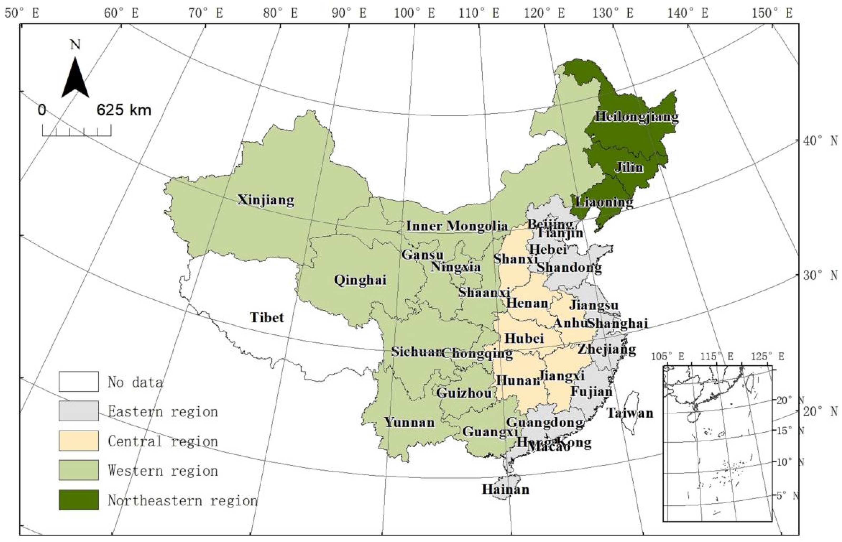
Figure 1. The schematic diagram of the four economic zones of China.
Water 14 02908 g001
Figure 2. The annual average WRGUE of each province during 2009–2019.
Water 14 02908 g002
Figure 3. The Moran scatterplot maps of WRGUE in 30 provincial administrative units in 2009.
Water 14 02908 g003
Figure 4. LISA of WRGUE in 30 provincial administrative units in 2009.
Water 14 02908 g004
Figure 5. The Moran scatterplot maps of WRGUE in 30 provincial administrative units during in 2019.
Water 14 02908 g005
Figure 6. LISA of WRGUE in 30 provincial administrative units in 2019.
Water 14 02908 g006
Table 1. WSGUE assessment indicators.
Primary IndicatorsSpecific IndicatorsMeanMinMax
Input indicatorsThe total water consumption (108 tons)201.195222.5619.1
The capital stock (RMB 108 Yuan)130,946.57982.3530,575
The social employee (104 person)2719.8303.267150.25
Desirable output indicatorGDP (RMB 108 Yuan)19,083.8939.787,731.7
Undesirable output indicatorThe COD of wastewater (104 tons)50.621.97198.3
The nitrogen of wastewater (104 tons)5.060.123.09
Table 2. WSGUE assessment indicators.
Explanatory VariableVariables’ Definition and UnitPre-Judgment
Economic development levelPer capita GDP (RMB 104 Yuan)Positive
Water resources use structureProportion of agricultural water to the total water consumption (%)Negative
Technical progress levelProportion of R& D expenditure to GDP (%)Positive
Opening-up levelProportion of the foreign trade to GDP (%)Positive
Urbanization levelProportion of the urban population to the total resident (%)Unknown
Population densityResident population per square kilometer (person/sq.km)Unknown
Table 3. The regression results of Likelihood ratio test and Wald test.
Fixed EffectsRandom Effects
Wald test spatial lag46.56 ***112.08 ***
LR test spatial lag42.80 ***80.20 ***
Wald test spatial error27.99 ***53.92 ***
LR test spatial error34.12 ***77.79 ***
Note: *** represents p < 0.01.
Table 4. The VIF test.
InDELInWSUSInTDLInOPLInULInPDMean VIF
VIF5.441.743.322.765.813.473.76
1/VIF0.1840.5750.3010.3620.1720.288
Table 5. The values of WRGUE for 30 provincial administrative units in China from 2009 to 2019.
Regions20092010201120122013201420152016201720182019Mean
Beijing1.0001.0001.0001.0001.0001.0001.0001.0001.0001.0001.0001.000
Tianjing0.5810.5950.6290.5840.6560.6660.6101.0040.5550.6270.5950.646
Hebei0.3870.3810.3840.3520.3820.3680.3550.3680.3320.3360.3310.362
Shanghai1.0001.0001.0001.0001.0001.0001.0001.0001.0001.0001.0001.000
Jiangsu0.5580.5670.5750.5390.6050.6200.6070.6810.5610.5800.5480.586
Zhejiang0.6350.6410.6390.5710.6360.6230.5980.6320.5480.5710.5580.605
Fujian0.5710.5790.5620.5070.5620.5410.5090.5500.4730.4700.4560.525
Shandong0.4950.4900.4860.4540.4960.4950.4740.5010.4540.4690.4720.481
Guangdong0.8190.8230.7920.6920.7940.7750.7220.8020.6610.6480.6100.740
Hainan0.4470.4590.4450.3860.4220.4000.3670.3850.3290.3190.3050.388
Eastern region0.6490.6530.6510.6090.6550.6490.6240.6920.5910.6020.5880.633
Shanxi0.4430.4360.4410.4020.4360.4150.3790.3750.3550.3680.3620.401
Anhui0.3520.3610.3590.3350.3630.3550.3360.3820.3240.3150.3060.344
Jiangxi0.3360.3390.3340.3140.3400.3350.3210.3310.3010.2970.2870.321
Henan0.4170.4220.4330.3920.4400.4380.4150.4430.3830.3900.3760.414
Hubei0.4670.4750.4740.4280.4710.4570.4270.4670.4000.3900.3780.439
Hunan0.4440.4530.4520.4040.4510.4390.4080.4350.3820.3710.3550.418
Central region0.4100.4140.4150.3790.4170.4060.3810.4050.3580.3550.3440.390
Inner Mongolia0.3930.3970.3980.3740.4190.4100.4020.4760.4030.4410.4320.413
Guangxi0.3570.3520.3540.3140.3480.3360.3100.3300.2750.2640.2460.317
Chongqing0.3960.4140.4400.4230.4710.4740.4670.6400.4780.5350.5160.478
Sichuan0.3700.3830.4040.3700.4150.4040.3800.4070.3660.3640.3550.383
Guizhou0.4310.4310.4330.3830.4250.4030.3710.3820.3250.3100.2920.381
Yunnan0.4130.4140.4120.3740.4190.4010.3760.4150.3540.3440.3280.386
Shaanxi0.3970.4050.4190.3960.4290.4240.4060.4230.3900.4040.4010.408
Gansu0.3690.3650.3610.3190.3540.3360.3070.3530.2870.2860.2780.329
Qinghai0.3330.3310.3340.3110.3250.3080.2880.2930.2780.2760.2700.304
Ningxia0.3260.3210.3220.2930.3170.3090.2950.3150.2780.2760.2640.301
Xinjiang0.4090.4000.3940.3370.3770.3620.3270.3430.2840.2790.2620.343
Western region0.3810.3830.3880.3540.3910.3790.3570.3980.3380.3440.3310.368
Liaoning0.3850.3880.3980.3730.4080.4030.3980.4530.3890.4040.4020.400
Jilin0.2890.2910.2900.2830.3090.3060.2910.3280.2890.2910.2830.296
Heilongjiang0.3880.3840.3730.3240.3560.3440.3210.3550.3020.2960.2860.339
Northeast0.3540.3540.3540.3270.3580.3510.3370.3790.3270.3300.3240.345
China0.4740.4770.4780.4410.4810.4720.4490.4960.4250.4310.4180.458
Table 6. Value of Global Moran’s I of provincial WRGUE in China (2009–2019).
YearGlobal Moran’s IZ-Scorep-Value
20090.224 **2.2490.025
20100.237 **2.3550.019
20110.247 **2.4460.014
20120.231 **2.3750.018
20130.251 **2.4650.014
20140.263 ***2.5670.010
20150.254 **2.5220.012
20160.297 ***2.7750.006
20170.208 **2.1580.031
20180.236 **2.3620.018
20190.225 ***2.2940.022
Note: *** represents p < 0.01, ** represents p < 0.05.
Table 7. The regression results of SDM.
Spatial Fixed-EffectsTime Fixed-EffectsSpatial and Time Fixed-Effects
InDEL0.8086419 ***0.7220803 ***0.6974106 ***
InWSUS0.0004369−0.0032236−0.0004647
InTDL0.0937041 ***0.00393240.0824482 **
InOPL0.0625741 ***0.01254810.0717951 ***
InUL−0.9996273 ***−0.2393367 ***−0.9468609 ***
InPD−0.02957990.1158211 ***−0.1191172
W*InDEL−0.8510972 ***−0.4911258 ***−1.53070 ***
W*InWSUS−0.0068093−0.0752403 ***0.0045217
W*InTDL−0.0155968−0.1458118 **0.014417
W*InOPL−0.01669940.1628485 ***0.0597447 *
W*InUL0.9070408 ***−0.08683071.122323 ***
W*InPD−0.3018763−0.0216836−0.9419549 ***
Variance sigma2_e0.0030164 ***0.0136224 ***0.0024756 ***
R-squared0.35620.00100.2760
Log-likelihood472.5766240.4700521.8122
Note: ***, **, and * indicate significance at the 1%, 5% and 10% levels, respectively.
Publisher’s Note: MDPI stays neutral with regard to jurisdictional claims in published maps and institutional affiliations.