Article

Flood Frequency Estimation in Data-Sparse Wainganga Basin, India, Using Continuous Simulation

UK Centre for Ecology & Hydrology, Wallingford OX10 8BB, UK
*
Author to whom correspondence should be addressed.
Water 2022, 14(18), 2887; https://doi.org/10.3390/w14182887
Submission received: 10 August 2022 / Revised: 8 September 2022 / Accepted: 9 September 2022 / Published: 15 September 2022
(This article belongs to the Section Hydrology)

Abstract

:
Monsoon-related extreme flood events are experienced regularly across India, bringing costly damage, disruption and death to local communities. This study provides a route towards estimating the likely magnitude of extreme floods (e.g., the 1-in-100-year flood) at locations without gauged data, helping engineers to design resilient structures. Gridded rainfall and evapotranspiration estimates were used with a continuous simulation hydrological model to estimate annual maximum flow rates at nine locations corresponding with river flow gauging stations in the Wainganga river basin, a data-sparse region of India. Hosking–Wallis distribution tests were performed to identify the most appropriate distribution to model the annual maxima series, selecting the Generalized Pareto and Pearson Type III distributions. The L-moments and flood frequency curves of the modeled annual maxima were compared to gauged values. The Probability Distributed Model (PDM), properly calibrated to capture the dynamics of peak flows, was shown to be effective in approximating the Generalized Pareto distribution for annual maxima, and may be useful in modeling peak flows in areas with sparse data. Confidence in the model structure, parameterization, input data and catchment representation build confidence in the modeled flood estimates; this is particularly relevant if the method is applied in a location where no gauged flows exist for verification.

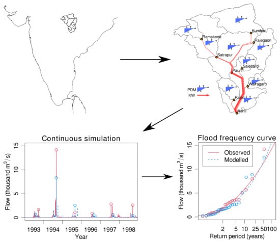
Graphical Abstract

1. Introduction

The summer monsoons experienced in peninsular India lead to regular, significant flooding over wide areas. With the rapid expansion of cities such as Mumbai putting further pressures on the river and drainage network, more extreme flooding has occurred in recent years, affecting millions of people. This century, Mumbai has seen extreme floods in 2005 and 2017 [1], and Ahmedabad in Gujarat experienced floods in July 2015 with over 70,000 m3/s extra flow released from Dharoi dam on the Sabarmati (a tributary of the Krishna), affecting up to 4 million people [2].
Most of the research in the region regarding extreme events and monsoon behavior is focused on flash flood prediction with short lead times (e.g., [3,4]). However, in terms of civil engineering projects and settlement planning, long return period (e.g., 100-year) flood frequency estimation is invaluable to ensure the suitability of flood defenses, irrigation and hydropower generation projects. In order to perform this estimation and allow it to be used more widely, the availability of the data must be considered.
The Central Water Commission (CWC) in India has developed many flood frequency estimation methods, with separate calibration in many different sub-zones of India (e.g., [5,6,7]). Through this work, catchment descriptor equations making use of area, catchment slope, river length and event rainfall depth were developed for the 25-, 50- and 100-year return period floods using multiple linear regression.
Various non-dimensional methods have also been investigated to estimate long return period flood magnitudes [8], primarily using moments of the annual maxima data and a “shape” parameter (area divided by squared channel length) fitted using linear regression. Rainfall for storm events determined through a depth-duration-frequency relationship is often used to model flood frequency relationships across India [9,10]. Typically, these studies have focused on estimating the mean of the annual maximum (AMAX) series, QBAR. More recently, machine learning has been applied to develop Bayesian decision-tree models to use catchment descriptors to estimate the median of the AMAX series, QMED [11]. In a different approach, a continuous gridded hydrological model was used to estimate QMED in the UK, which was verified at 550 river gauging stations [12].
The objective of this study is to test continuous simulation rainfall-runoff modeling as a method to estimate AMAX flows, from which flood frequency curves (FFC) can be generated in order to provide estimates of the magnitudes of long return period floods to stakeholders, so that their effects can be planned for, in reservoir design, for example. Unlike statistical analysis of gauged flows, continuous simulation rainfall-runoff modeling has the potential to be applied at ungauged sites. The main focus is on reproducing AMAX flows, rather than the whole flow regime, accurately, as AMAX are most commonly used to develop FFC. Furthermore, accurate reproduction of the whole flow regime may not be possible at this time as the daily flow data are not naturalized and are subject to significant artificial influence in the form of dams and other water management schemes [13]. In this study, we focus on the Wainganga basin, a ~50,000 km2 sub-basin of the Krishna basin in central mainland India with just nine permanently gauged sites that is increasingly being dammed for irrigation and hydropower.
This paper proceeds as follows. In Section 2, the study region is described, the available data are highlighted and the hydrological modeling procedures are outlined with their relative advantages and drawbacks. Section 3 first explains the statistical investigation used to choose an appropriate probability distribution to describe annual maximum flows in the region, then illustrates the flood frequency estimation results. Conclusions are presented in Section 4.

2. Materials and Methods

2.1. Study Region

The Wainganga River is a tributary of the Godavari River, originating near Gopalganj in the state of Madhya Pradesh. It flows for a length of approximately 600 km before joining the Wardha River just south of Chamorshi in the state of Maharashtra (Figure 1a).
The Wainganga basin (Figure 1b) is sparsely populated. Nagpur (population 2.4 million), near the Satrapur river gauging station and partly outside the Wainganga basin, is the only major city. Chhindwara and Gondia are the only other cities in the basin with a population above 100,000 as of 2011. Chandrapur (population 320,000) lies just outside the basin on its diagonal south-west side, at a similar latitude to the Rajoli river gauging station (Figure 1b). Heavy forests dominate the Wainganga valley, including the major tiger reserves Tadoba Andhari (Maharashtra) and Pench (Madhya Pradesh), which are themselves connected with other reserves inside and outside the basin via 16,000 km2 of undisturbed landscape [14] covering approximately one-third of the basin.
The Wainganga River is increasingly being dammed, replacing the forest cover with water [13,15]. The vast majority of dams are for irrigation, but an increasing number are being proposed for hydropower, such as the multi-dam Wainganga Hydroelectric Project [16]. The basin has been identified by India’s Marine Engineering and Research Institute (MERI) as “of interest” with regards to flooding.
This study considers the Wainganga basin to Ashti gauging station, a few kilometers upstream of the junction with Wardha. The Wainganga catchment to Ashti gauging station has an area of approximately 51,500 km2. Nine sub-catchments are considered, each directly upstream of a gauging station and therefore not necessarily near a confluence. The nine sub-catchments range from approximately 1750 to 36,000 km2 in area.

2.2. River Discharge Data

The CWC and Indian Meteorological Department (IMD) have over 900 flow gauging stations that measure river stage, discharge, water quality and sediment content, although most stations only measure a sub-set of these. Most of the discharge is estimated by CWC using an area-velocity method with autographic water level recorders, except in very high flow when slope-area methods are used to estimate discharge. In some periods, missing observations are filled with estimates that match the general day-on-day trend of the discharge. Daily gauge data were available from the India-WRIS web portal [17] for periods of between 2 and 40 years per station, from which annual maxima can be determined. Locations of the nine gauging stations in the Wainganga basin (Figure 1b) were obtained, and HydroSHEDS terrain elevation data (outlined in Section 2.3) was used with GIS software to determine the upstream catchment boundary.
Within the Godavari and Krishna basins, 122 river discharge stations (including the 9 in the Wainganga basin) were identified as suitable to determine appropriate distributions to develop flood-frequency relationships from the AMAX series. Stations were considered suitable if they had less than 10% missing data during the monsoon season over their period of record. It is noted that some stations only operated around the monsoon season, not continuously over the whole year.

2.3. Elevation and Flow Direction Data

The HydroSHEDS [18] and HydroBASINS [19] datasets consist of “hydrologically corrected” elevation data on a 3 arcsecond resolution (approximately 90 m at the equator), along with flow direction and accumulation data on a 15 arcsecond resolution. These products rely mostly on Shuttle Radar Topography Missions outputs and topographic maps. Hydrological conditioning includes several procedures that force the correct river network topology into the DEM [20] (pp. 10–13). This dataset was used to determine the shape and size of the watersheds that drain into the gauging stations, and from this, which cells in the gridded meteorological datasets (Section 2.4) related, fully or partly, to each Wainganga sub-catchment. The DEM was also used to further characterize the sub-catchments in terms of area, average slope and average elevation.
Water bodies were obtained from HydroLAKES [21], which includes all water bodies of area 105 m2 or greater, linked to be consistent with the main HydroSHEDS DEM. HydroLAKES data in India are derived from two sources: SRTM Water Body Data [22], generated as a by-product of the SRTM, and the Global Reservoir and Dam (GRanD) dataset, v1 [23,24], which notes more than 100 reservoirs in India. This dataset includes natural lakes and does not include some recent major reservoirs, such as that created by Gosekhurd Dam, near Pauni gauging station, with an effective storage capacity of 7.40 × 10⁸ m3 and a reservoir area of 222 km2 [15].

2.4. Meteorological Data

The production of a simulated flow record for each sub-catchment required rainfall and evapotranspiration records as input data to the hydrological model. Rainfall data were derived from a gridded IMD dataset [25], providing daily rainfall totals for all of India over the period 1901–2015 at 0.25° spatial resolution. The Climate Hazards Group InfraRed Precipitation with Station data (CHIRPS) dataset, version 2.0 [26], was considered as an alternative to the IMD dataset due to its higher spatial resolution (0.05°) and augmentation of rain gauge data with satellite data. It was initially assumed that both of these advantages would allow CHIRPS to detect higher-intensity rainfall features. However, a comparison of 1-day annual maxima from both datasets over their common period of 1981–2015 shows that IMD normally records the larger 1-day maximum, even though CHIRPS records the larger annual total. For this reason, IMD was preferred over CHIRPS. Average annual rainfall (1981–2017) in all study sub-catchments is very similar (minimum = 1264 mm, maximum = 1391 mm).
Evaporation data were derived from the GLEAM dataset, version 3.3a [27,28], at daily temporal and 0.25° spatial resolution for the period 1980–2018. Potential evaporation for bare soil, short canopy and tall canopy were estimated using observations of surface net radiation and near-surface air temperature with the Priestley–Taylor equation. This was converted to actual evaporation through observations of microwave vegetation optical depth and estimated root-zone soil moisture, via water balance. GLEAM data are modeled estimates, not observed.

2.5. Land Cover Data

Land use and land cover data were obtained from the Harmonized World Soil Database, version 1.21 [29]. This divides the world into grid cells of (1/12)° resolution and assigns one of seven categories to each grid cell: rain-fed cultivated land, irrigated cultivated land, forest land, grass/scrub/woodland, built-up land, barren/very sparsely vegetated land and water body. Table 1 provides broad, statistical information on the nine gauging stations and their upstream catchments. DPLBAR (mean drainage path length) and DPSBAR (mean drainage path slope) are equivalent to the FEH catchment descriptors of the same name [30], derived from HydroSHEDS river network data. CULT, URB and FOR express the fraction of each sub-catchment belonging to the HWSD Land Use and Land Cover categories of the same names, indicating “total cultivated land”, “built-up land” and “forest land”, respectively.

2.6. Statistical Flood Frequency Estimation

To compare observed and modeled flood frequency, AMAX series are extracted from the observed flow and modeled flow, and flood frequency curves (FFC) are plotted for both, using the same distribution. Therefore, an appropriate distribution for the AMAX must be selected.
To determine an appropriate distribution, a Hosking–Wallis test was performed using the L-moment ratios and the ZDIST statistic [31,32] on the whole dataset using the lmomRFA package from R [33,34].
For each catchment, the ZDIST statistic was calculated as:
ZDIST = [(τ4 − τ4DIST) − B4]/σ4
where τ4 is the sample L-kurtosis, τ4DIST is the expected L-kurtosis under the chosen distribution, derived as a function of the sample L-skew, B4 is a bias correction term, the sample mean of a set of simulated copies of (τ4 − τ4DIST), and σ4 is the sample standard deviation of the copies. Any distribution with a value of |ZDIST| < 1.64 was deemed to be potentially acceptable for that station. The distribution with the smallest value of |ZDIST| was also recorded, this being referred to as the “chosen” distribution for that station.

2.7. Hydrological Model

In this study, catchment runoff was modeled using the PDM (Probability Distributed Model) [35]. This is a lumped, conceptual rainfall-runoff model with three storage elements representing soil (Pareto distribution), surface storage (linear reservoir) and groundwater storage (cubic reservoir), respectively. The soil store is fed by rainfall and depleted by evapotranspiration, recharge and saturation-excess runoff. Recharge is fed into the groundwater store, saturation-excess runoff is fed into the surface store. Outflows from the groundwater and surface stores combined give the catchment outflow.
Initially, each of the nine sub-catchments of the Wainganga basin was modeled in a lumped configuration. This means that each catchment included all upstream sub-catchments. For example, lumped modeling of the catchment to Ashti included the entire upstream area, enclosing the other eight gauging stations. However, the upstream stations were effectively ignored, as their data were not used in calibration or validation (initially).
After lumped modeling, semi-lumped configurations of non-overlapping sub-catchments with flow at each upstream gauge translated to the next downstream gauge using kinematic wave (KW) routing were produced for Ashti, Pauni and Satrapur. KW routing has one parameter, the wave speed, c. When a river channel is divided into segments, the wave speed controls how much water moves from one segment to the next during one time step. Semi-lumped in this context means that each sub-catchment PDM and channel was modeled using the same parameters.
Lumped, semi-lumped and semi-distributed modeling each have their own advantages and disadvantages. Lumped modeling of one catchment benefits from being able to use the entire period for which precipitation, evapotranspiration and verification data are available at one station, while semi-lumped and semi-distributed modeling can only use the period for which these data are available simultaneously at all stations. However, lumped modeling cannot account for spatial differences in precipitation across a catchment: an intense rainfall event near the gauging station could reasonably be expected to generate a more rapid rise and fall in gauged flow than one in the headwaters. Lumped modeling can only account for very different soil and land-use types conceptually, through the use of parallel stores, each of which the model stipulates must necessarily receive the same rainfall depth per timestep. Semi-lumped modeling can account for spatial rainfall variations, but not different catchment properties, as the same PDM parameters are used for all sub-catchments. Semi-distributed models can account for spatial variations in rainfall, soils and land use, but require different parameter values for each sub-catchment, making them very difficult to parameterize. Linking parameter values to measurable sub-catchment properties can simplify calibration greatly, as each model parameter at each sub-catchment becomes expressible as an equation with a single set of optimized coefficients applicable to every sub-catchment. However, measurable properties cannot explain all of the variance in parameter values, so parameter values calculated in this way are never optimal, even if they may be acceptable.

2.8. Model Calibration and Validation

In all cases, PDM parameter values were optimized to maximize the modified KGE (Kling-Gupta Efficiency) [36] of the simulated river flow relative to that observed, in units of mm/day. Modified KGE is a performance metric that compares two time-series in terms of three components:
KGE’ = 1 − [(r − 1)2 + (β − 1)2 + (γ − 1)2]½
β = μso
γ = (σss)/(σo/μo)
where KGE’ is the modified KGE statistic, r is the Pearson correlation coefficient, β is the bias ratio and γ is the variability ratio (all dimensionless). Subscripts s and o indicate simulated and observed values, respectively. Note that KGE’ values range from to 1 and values closer to one show better performance. Throughout this study, the first three years of simulated river flow were discarded and KGE’ was maximized on the remaining paired simulated and observed data points. Throughout this study, optimal parameter sets were found using a shuffled complex evolution algorithm [37,38].
Typically, a continuous simulation model is desired to be equally accurate across the whole range of modeled flows, and both the objective function and range of data used for calibration reflect this. Within Section 3.2 and Section 3.5, the full time-series at each station (excluding the first three years) was used to calibrate the PDM through maximization of KGE’ at each station separately. Section 3.5 imposed the constraint that only a single value for each parameter can be fitted to all stations; this value was found through optimization of the mean KGE’ across all stations. In Section 3.6, semi-lumped models were produced for the three non-headwater catchments, and the PDM and kinematic wave speed were optimized to maximize KGE’ between the full observed and simulated time-series at the outlet (excluding the first three years).
If certain flows are considered more important than others, these can be weighted more highly in the objective function, and less important flows can be ignored. As the purpose of these models is to improve estimation of annual maximum flows, an objective function maximizing KGE’ on only the annual maximum flow series was tested for its ability to recreate the observed flood frequency curve for each station (Section 3.3). This was tested against conventional (e.g., Section 3.2) calibration in a split-sample test in Section 3.4.
The CWC’s flood frequency estimation procedure for the Lower Godavari sub-zone [5], which includes the Wainganga basin, is broadly applicable to catchments up to 1000 km2. Since the smallest sub-catchment in this study measures 1755 km2, and most are over 5000 km2, it is not appropriate to compare the CWC’s method to the one tested in this study. Methodological validation is conducted against gauged data only.
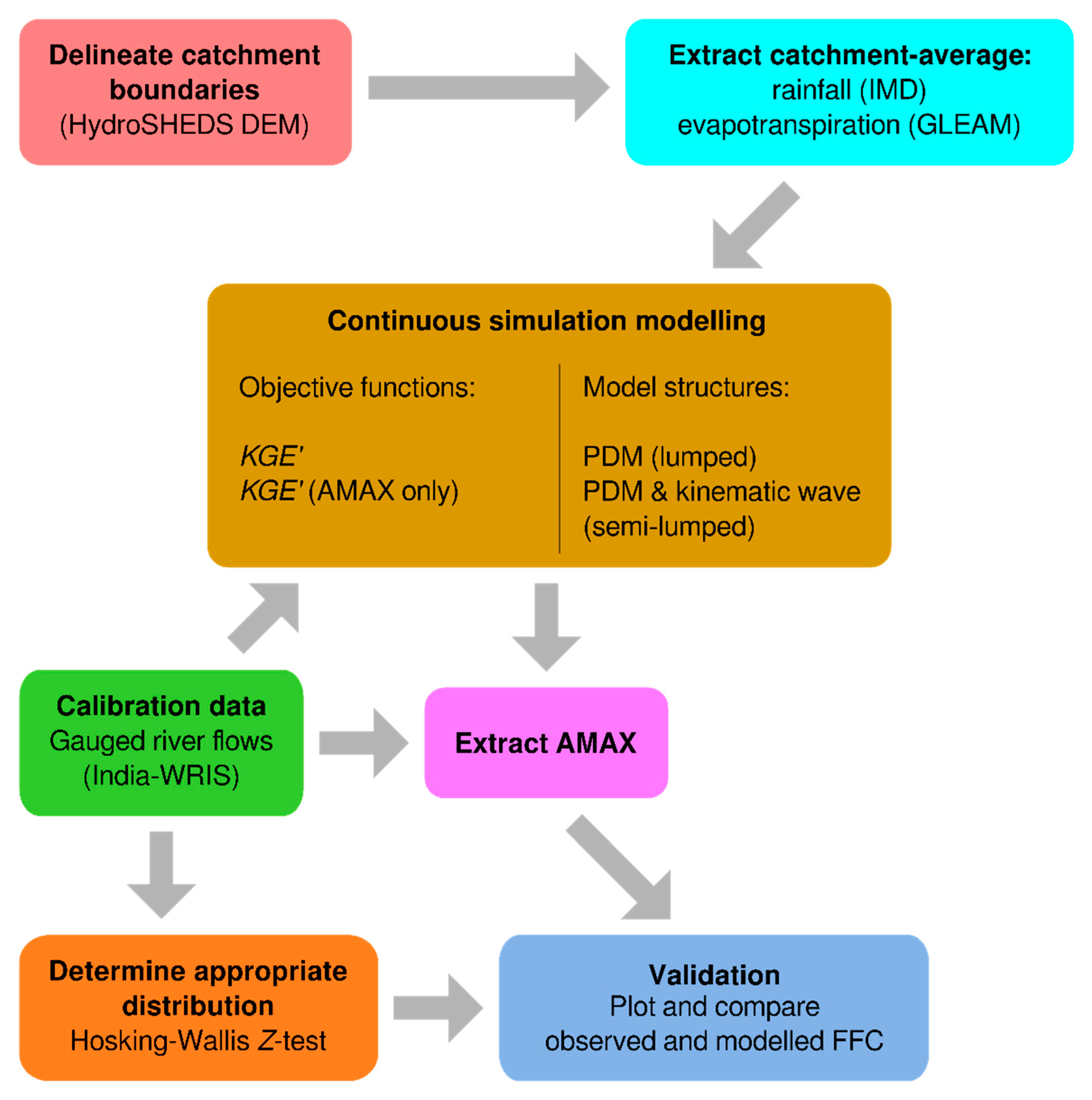
Figure 2 depicts the study methodology, including catchment delineation, data preparation, river flow model frameworks, optimization functions, preparation of gauged verification data and development of flood frequency estimates.

3. Results and Discussion

3.1. Distribution Choice

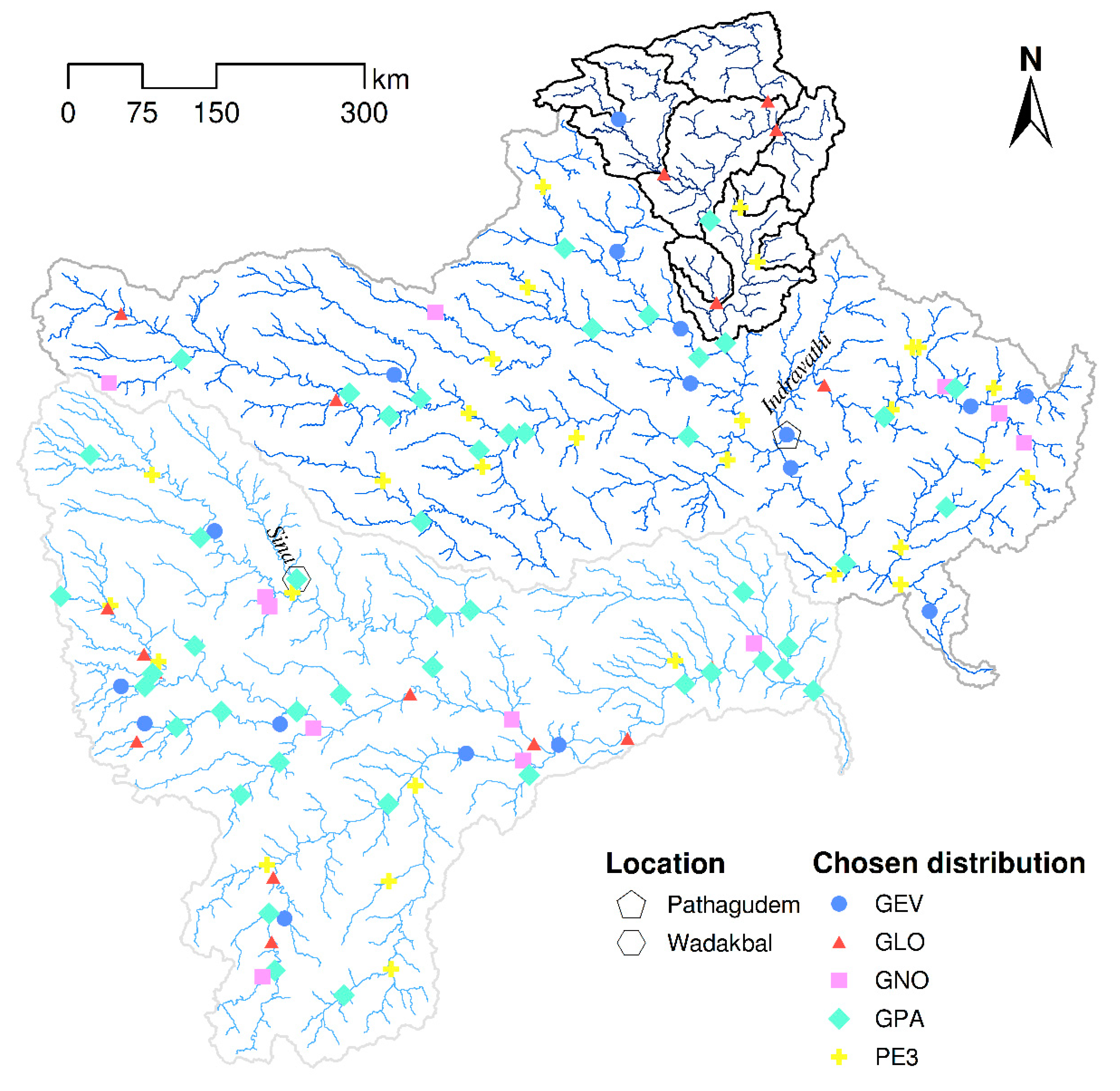
Figure 3 shows the chosen distribution at each of the gauging stations in the dataset, and Table 2 shows total stations at which each distribution was acceptable and chosen. Although the Generalized Pareto (GPA) is most often the best distribution, the Pearson Type III (PE3) is the most frequently acceptable. No obvious spatial correlation to the choice of distribution is visible; these patterns do not match the major river channels or major topographical features. Within the Wainganga basin, the GPA distribution was acceptable at all nine stations and the PE3 distribution was acceptable at seven. However, only two chose PE3 as the best distribution, and another two chose GPA. Generalized Logistic (GLO) and Generalized Extreme Value (GEV) were also chosen by four and one Wainganga stations, respectively.
Theoretically, under certain assumptions, all block maxima series, such as the series of annual maximum river flows, follow the Generalized Extreme Value Distribution (GEV). However, this and other studies into the optimal choice of distribution in regions of India have recommended the use of other distributions. The acceptability of the GPA distribution for AMAX flows is variously supported [39,40] and contradicted [41,42,43] by previous studies on much smaller datasets of 4 to 18 Indian stations.
In Kerala, south-west India, the Chi-square test, ranking of statistical indicators and the L-moment ratio diagram highlighted the Generalized Pareto (GPA) and Generalized Logistic (GLO) distributions for at-site analyses [39]. In the Tel basin in the Mahandi river system in east India, Guru and Jha [40] considered four stations and, via Kolmogorov–Smirnov tests, found the GPA to fit best to annual maxima data and the Generalized Log-Normal (GLN) to fit best to peak-over-threshold data. However, Swetapadma and Ojha [41], also studying the Mahanadi river system, selected the GEV distribution as the best-fitting to AMAX data at 18 stations. The Lower Godavari sub-zone was investigated using artificial neural network methods [42], and the Pearson Type III (PE3) highlighted through Hosking–Wallis tests as an appropriate distribution. In the Middle Ganga Plains in India, Kumar et al. [43] used Hosking–Wallis tests to first identify eight (of eleven) sites as one homogeneous region, then selected the GEV distribution for that region.
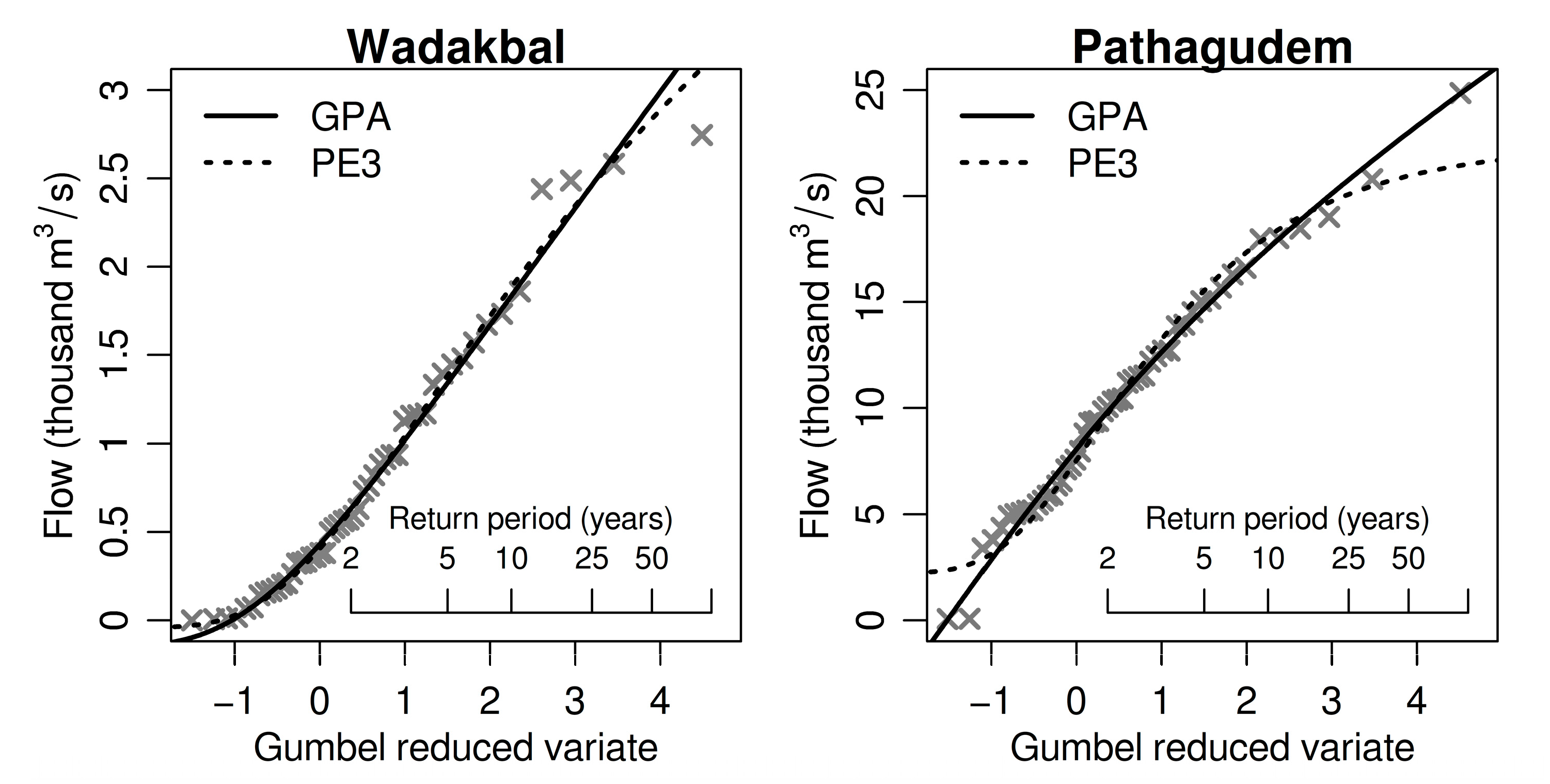
In Figure 4, two examples are shown to discuss features of the Generalized Pareto and Pearson Type III distributions and how well they fit in different areas of the study region. The Gumbel reduced variate is used to better distinguish the empirical return periods at the lower and upper limits.
Firstly, Wadakbal on the Sina River is a catchment of area 12,010 km2, upstream of the Krishna near the Western Ghats. This dry catchment receives an average annual rainfall of 1053 mm, and consists primarily (73%) of cultivated, irrigated land. At its most extreme, almost no flow can be seen in the Sina for multi-year periods, and as such, even the annual maximum can nearly reach zero. In this case, Figure 4 shows that both the GPA and PE3 distributions fit similarly, and this is frequently true for the drier catchments, typically found towards the west of the Krishna and Godavari basins.
On the other hand, Pathagudem is a catchment of area 39,227 km2 on the Indravathi River in the lower reaches of the Godavari, located towards the east coast of peninsular India. Its larger area in part accounts for the higher discharge, as does the higher average annual rainfall of approximately 1800 mm, a direct result of the seasonal monsoons. This region is also 60% forested due to this climate. In this case, the apparent lower bound to the AMAX series seen in Figure 4 (except for two outliers) may be due to this large amount of somewhat predictable rainfall. Here, we see that the Generalized Pareto distribution captures the magnitude of the most extreme events at both tails. On the other hand, the PE3 distribution fits the central behavior very well, which still allows reasonable estimation up to the 1-in-25-year flood, but does not capture the behavior of tails as well. Therefore, this paper uses the GPA distribution, since it was accepted by all the Wainganga stations under the Hosking–Wallis test, and the climate in the Wainganga basin is more similar to Wadakabal than to Pathagudem.

3.2. Lumped Sub-Catchment Modeling

Table 3 presents modified Kling-Gupta efficiency (KGE’), its decomposed components and the Nash–Sutcliffe Efficiency (NSE) for each station. The theoretical best value for each of KGE’, r, γ, β and NSE is 1.
The results here show that the PDM is in general appropriate for lumped sub-catchment modeling of the Wainganga basin, with a mean KGE’ of 0.612 across all nine stations. This extends existing confidence in continuous simulation modeling, which has generally focused on much smaller catchments [44,45,46]. The overall KGE’ values observed for these catchments depend most strongly on the Pearson product-moment correlation between observed and modeled flows as there is almost no volumetric bias for any catchment, and the reported values for the coefficient of variation component of the KGE’ show that the PDM only slightly underestimates flow variability in most cases. NSE values are generally much lower than KGE’ values, although NSE at Ashti is favorable in comparison to a recent study using the SWAT model [47]. Low or negative NSE values may indicate that observed flows are relatively stable, not that modeled flows are particularly poor [48]. However, the standard deviations of observed flows at the three stations with the lowest NSE values are all over 4 mm/day, compared with 2.5 mm/day at Pauni. At Kumhari and Ramakona, the means and standard deviations of the modeled flows were also similar to those observed, although at Wairagarh, they were underestimated. Wairagarh is also the catchment with the highest mean and standard deviation of observed flows (2.6 and 7.1 mm/day).
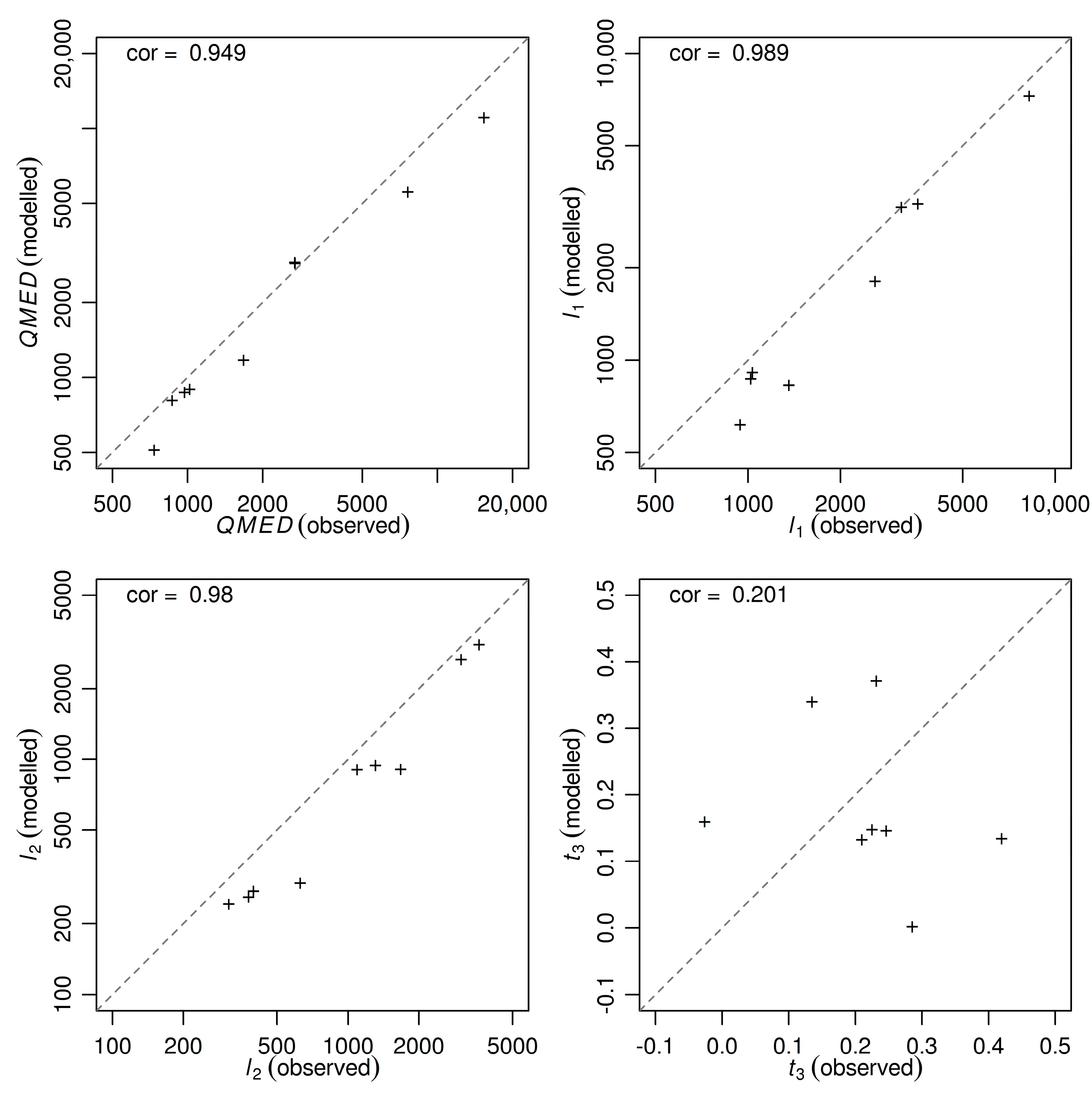
Despite the performance in KGE’ ranging from reasonable (0.333) to good (0.880), the calibration metric does not focus strongly on annual maximum flows. This is summarized in Figure 5, which shows very strong correlations between modeled and observed QMED, l1 and l2 (first two L-moments), but it has an obvious mild bias, particularly with less variability (l2) modeled than observed. It is expected that use of Nash–Sutcliffe Efficiency as an objective function would reduce the modeled flow variability further, as the KGE (and later KGE’) metrics were developed in response to the tendency of NSE to downplay the observed flow variability. Presumably, the slight underestimations in flow variability found for most catchments (those with γ < 1) relate to the most extreme values, i.e., the annual maxima and minima.
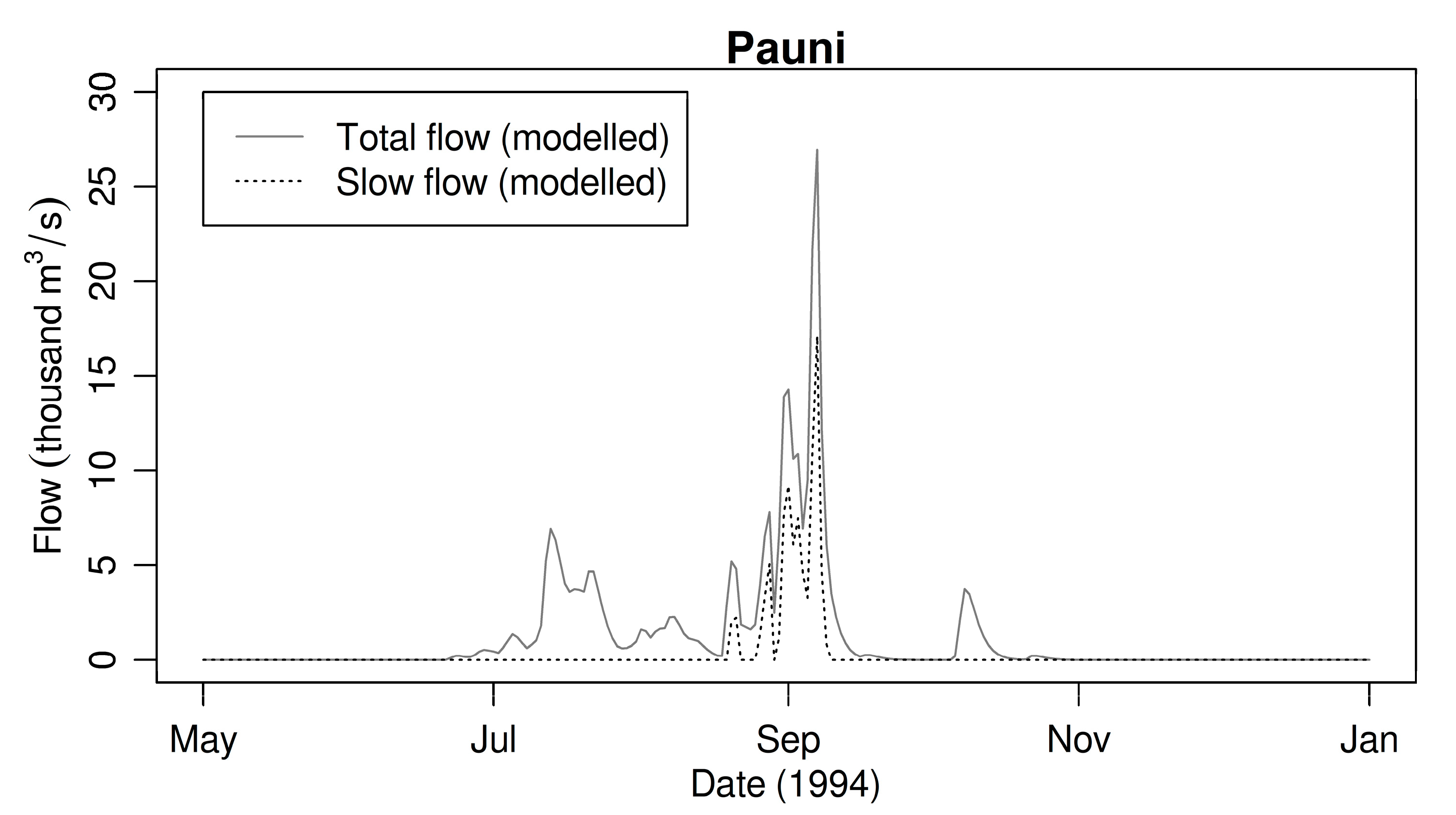
This is likely due to a number of factors. Firstly, if the gauged flows are poor or uncertain representations of reality, then the model may need to implement extreme parameterizations to produce modeled flows that closely match the poor or uncertain gauged flows. Secondly, poor-quality input datasets may mean that the model has to apply extreme transformations to the input rainfall and/or evapotranspiration to produce a modeled runoff similar to the gauged runoff. Thirdly, lumped modeling aggregates all rainfall and evapotranspiration spatially, meaning that an intense cloudburst near the catchment outlet is modeled in the same way as one occurring over the headwaters, even though the travel time to the gauging station, and the amount of attenuation occurring on the way there, is very different in both cases. However, hydrological models can attenuate input rainfall by a greater or lesser amount through parameterization, and both lumped and semi-distributed modeled runoff can be equally accurate [49,50]. Fourthly, if certain hydrological processes are absent from the conceptual model structure, then the processes that are present will try to compensate, but they may take extreme parameterizations to do so. One physically plausible but unmodeled process in the Wainganga basin may be reservoir storage, which could manifest in the model parameterization as an increased soil storage capacity. Indeed, cmax, the maximum soil storage capacity, takes a value of 5900 mm in Rajoli and 2500 mm in Satrapur, while the lowest value it takes is 800 mm in Wairagarh. Formal quantification of reservoir effects is complicated, as the interaction of each reservoir and catchment is unique in India [51]. Finally, equifinality (multiple ways to achieve the same answer) may mean that the same KGE’ can be achieved by more than one parameter set. Equifinality and unrepresented processes are linked, as there are two flow paths out of the PDM, a nominally “fast” and a nominally “slow” response. The fast response made up the vast majority of flow in all nine catchment models—neither Kumhari nor Rajegaon produced any modeled slow flow, and the model producing the most was Salebardi, at 14.3% of the total flow. However, the seven models that did produce slow flow all produced it similarly: drier years had no slow flow, while in wetter years, slow flow increased as the wet season progressed, and as a fraction of individually high peak flows. As a result, nominally slow flow contributed a considerable portion to the largest AMAX flows in Satrapur, Pauni and Rajoli. As there were no modeled dry-season flows for any catchment, no flow path modeled a baseflow-type flow, but both flow paths could and did contribute to peak flows (Figure 6).
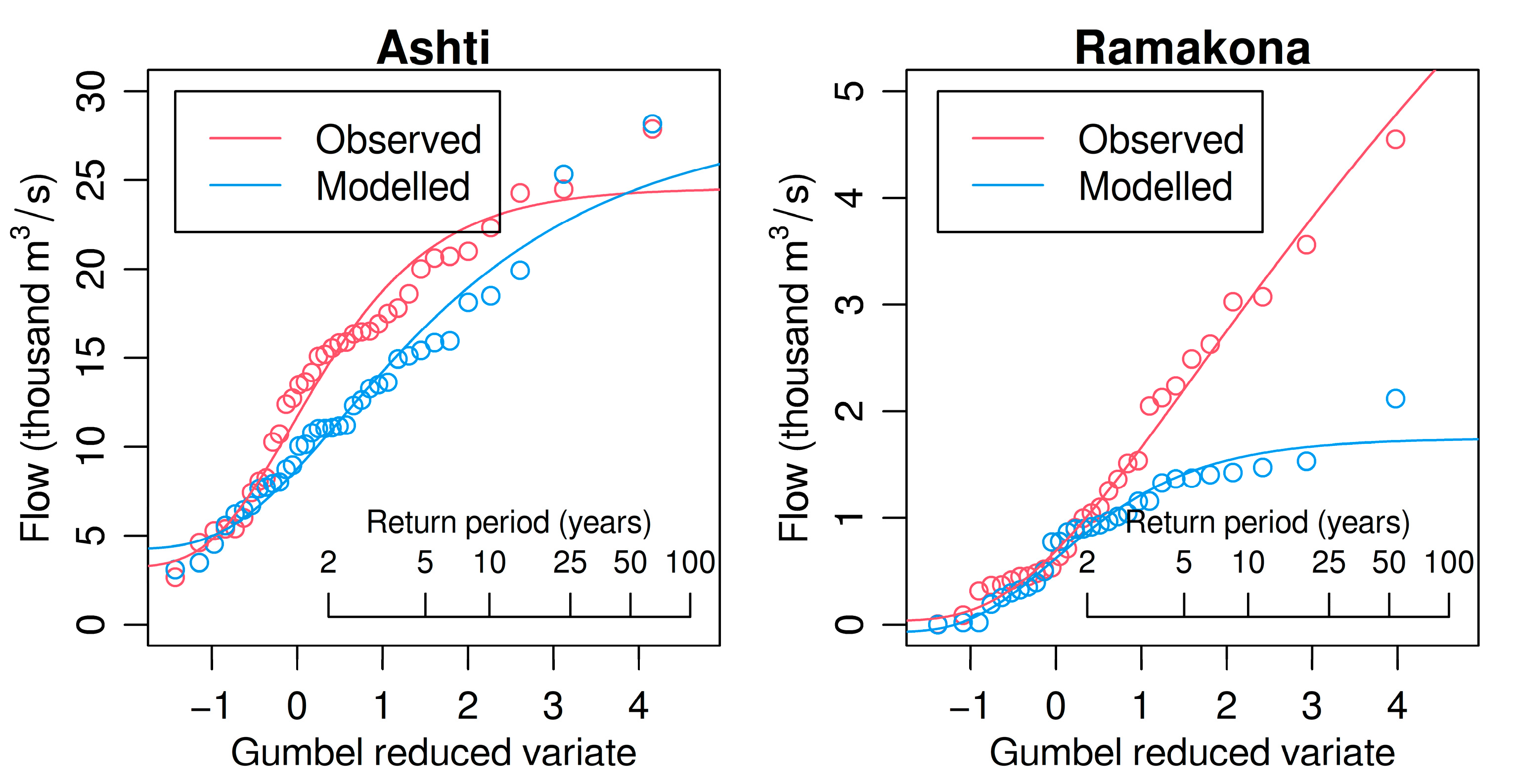
Reduced variability in the modeled flows can also be seen in the FFC produced by fitting a Generalized Pareto distribution to the observed and modeled AMAX. Examples are reproduced for Ashti (KGE’ = 0.880) and Ramakona (KGE’ = 0.333) in Figure 7.
The modeled AMAX and Generalized Pareto FFC at Ashti is clearly show reasonably low errors for floods with 25–100-year return periods. This ability to generate a viable FFC from continuous simulation is similar to that reported in a much smaller (8.41 km2) urban Australian catchment [45]. However, AMAXs at Ashti are consistently underestimated at shorter return periods. This consistent underperformance in modeling AMAX magnitude is perhaps unsurprising, as the KGE’ performance metric focuses on the whole flow hydrograph, of which only one point out of every 365 or 366 is an AMAX; this criticism is equally applicable to Nash–Sutcliffe efficiency and other time-series performance metrics. The consistent underestimation of the entire FFC at Ramakona may be related to the creation of the gridded rainfall data. Ramakona contains some very steep and mountainous areas, and it does not seem that elevation was included as a covariate in the rainfall interpolation process [25]. However, from a purely KGE perspective, the performance of the PDM at Ramakona, and across all nine Wainganga sub-catchments generally, is close to that of EPA-SWMM when applied to simulate continuous runoff from two rural, highly seasonal south Australian catchments of 27 and 122 km2 [46].

3.3. Lumped Sub-Catchment Modeling (Optimizing AMAX Performance Only)

In this test, KGE’ was maximized only between pairs of observed and modeled AMAX, in order to attempt to match better the values of interest for flood frequency estimation. A recent study [52] assessed nine different objective functions to better reproduce extremes; however, none of these applied higher weights to more relevant observations. Additionally, previous work [53] has considered bias correction to improve FFC derived through continuous simulation, and also used the fit between the observed and simulated FFC to calibrate the bias correction. However, maximization of KGE’ directly and exclusively on AMAX pairs could reduce or eliminate the need for FFC corrections.
Performance according to the KGE’ metric, its components and NSE, all computed on the full flow time-series (excluding years pre-1983), is shown in Table 4. Model configurations that are not optimized on the full time-series will not necessarily perform well on the full time-series. However, performance was particularly poor at Rajoli, with severely underestimated variability and overestimated total flow. Satrapur is the opposite: total flow was underestimated and variability was overestimated. For Wairagarh, bias and variability ratios were both close to the optimum, but correlation between values was not very high. Performance at Ashti and Pauni was arguably still good (in both cases, KGE’ ≈ 0.65, although γ and β were not very close to 1).
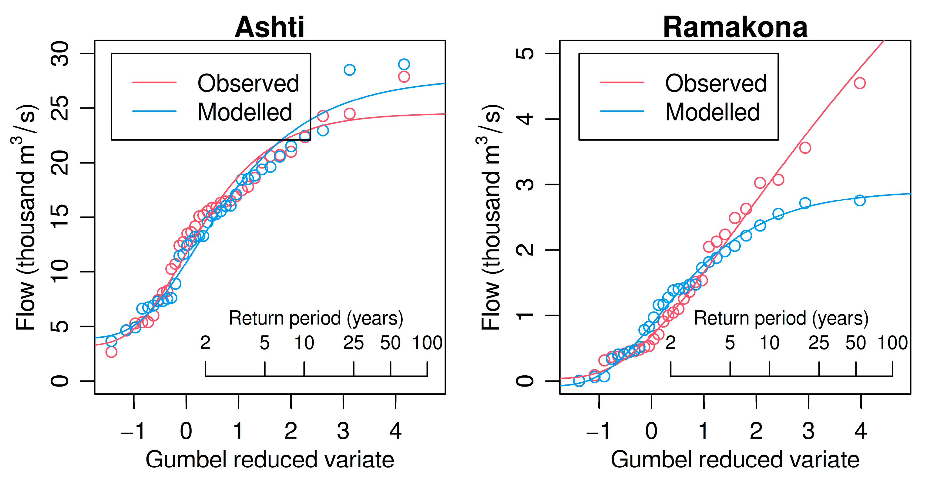
For comparison, the flood frequency curves generated for Ashti and Ramakona during this test are presented in Figure 8. Notably, the modeled and observed FFC for Ashti are near-identical, with the only major difference being for the second-largest AMAX. Despite the reduction in KGE’ from 0.330 to 0.160, the modeled AMAX at Ramakona are improved for events rarer than QMED. However, they are still largely unsuitable.

3.4. Lumped Sub-Catchment Modeling with a Calibration/Validation Period

Considering that the PDM is intended for continuous simulation of a catchment, it is suspected that a PDM optimized for something other than continuous simulation may behave unpredictably when presented with new data. On the other hand, a PDM that models continuous simulation reasonably well should behave predictably when presented with new data. If that predictability means that AMAX are underestimated, then they might be underestimated consistently, potentially allowing the development of post-processing rules to correct them. This cannot be guaranteed with a model that ignores the catchment processes on every day of the year except one, but it can be investigated by dividing gauged flow records into calibration and validation periods, using the AMAX objective function to calibrate the model and the calibrated parameters to estimate AMAX during the validation period.
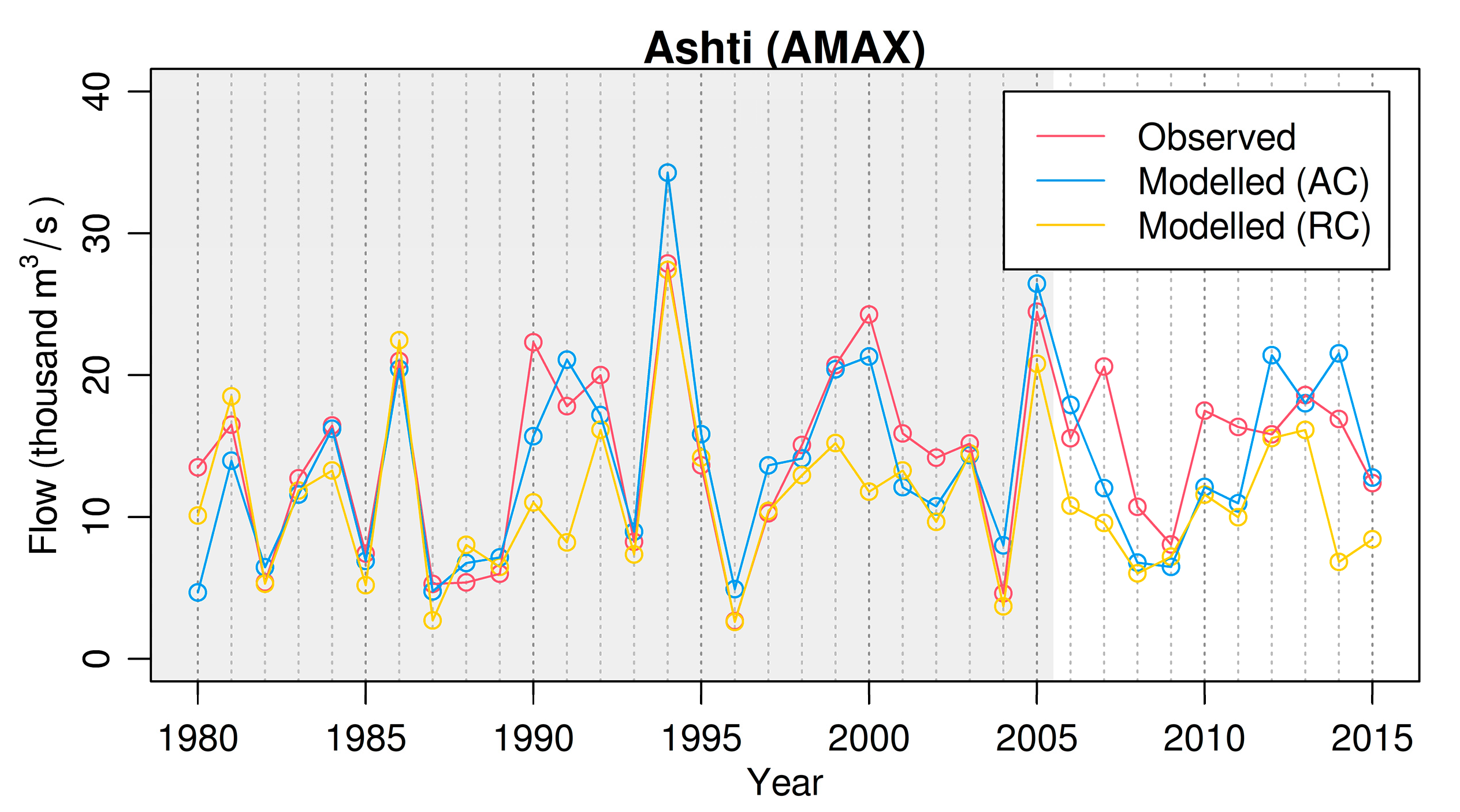
The gauged flow record for Ashti was divided into two parts, consisting of the final 10 complete years and the 26 years preceding them. The model parameters were fitted to minimize the error in estimated AMAX for years 1983–2006, ignoring three years for spin-up, then the calibrated model was applied to the whole record to estimate the final 10 AMAX. The observed and AMAX-calibrated (AC) modeled AMAX series for Ashti are plotted in Figure 9, alongside the full-flow-regime-calibrated modeled AMAX series (RC). RC uses the parameters determined in Section 3.3.
Qualitatively, the AC modeled AMAX are more closely matched during the calibration period than the validation period. However, it is a common for the performance of any model to decrease between calibration and validation periods. In fact, for AC, correlation between modeled and observed AMAX was 0.921 for the calibration period and 0.553 for the validation period, whereas the respective figures were 0.831 and 0.526 for RC. This indicates that the lower predictive performance of the AC model for the last 10 years is mainly due to other factors not related to its ability to predict AMAX when it is applied outside its calibration period.
These results suggest that it might be possible to use a PDM calibrated only to AMAX data to estimate AMAX outside of the calibration period, although this model will not be suitable for other purposes: the KGE’ of the AC model on the full flow series was just 0.458 for the calibration period and 0.388 for the validation period.

3.5. Lumped Sub-Catchment Modeling (Single Parameter Set)

In this test, optimization was performed on each lumped sub-catchment with the constraint that all nine sub-catchments must use the same parameter values. This gives guidance on how well a semi-lumped model (non-overlapping catchments with identical PDM parameterization), linked via kinematic wave routing (with identical wave speeds), might perform, without the extra work involved in setting up a KW routing scheme and network topology, and (if successful) greatly simplifies parameterization of the PDM for ungauged sub-basins of the Wainganga. The optimization was set to maximize mean KGE’ per catchment, with each catchment weighted equally. All monitored runoff time-series were trimmed to the longest possible common period: 18 July 1992 to 28 December 2014. While this trimming was not strictly necessary here, it is necessary for semi-lumped and semi-distributed modeling cases where flow is optimized at all gauging stations (note that the purpose of this model run is to evaluate the validity of continuing towards semi-lumped modeling). The flow was modeled over the full 1980–2015 period, hence allowing just over 12.5 years for spin-up. Because of this long spin-up, KGE’ was maximized over the full common period of gauged record.
Table 5 presents the performance metrics achieved for each catchment separately when modeling runoff with the optimized single parameter set over the period 1980–2015. In each case, the performance reported in Table 5 compares simulated and observed flows over the available flow data in the years 1983 to 2015 (as in Table 3 and Table 4).
Use of a single parameter set gave poorer model performance, with a mean KGE’ of 0.415 across all nine stations. Among individual catchments, Ashti and Pauni were the best modeled, as for all other variants of lumped modeling. As all sub-catchments were weighted equally, it is implied that the calibration data in these two are more accurate—as the largest catchments, they are the least mountainous proportionally. It may also be implied that the PDM more accurately represents the dominant flow processes for these two catchments. In contrast to the initial case, where parameter values were optimized individually for each catchment, values of the KGE’ components γ (variation) and β (bias) can vary wildly. The two catchments that performed most weakly with the single parameter set, Rajoli and Satrapur, were also those where the modeled flow total was far above the observed flow total (β is the highest). Rajoli was also the catchment with the lowest value of γ. These contributed to its low KGE’ value of just 0.001, despite the relatively high Pearson product-moment correlation coefficient of 0.612.

3.6. Semi-Lumped Modeling

Here, three separate semi-lumped models were considered: the Wainganga to Ashti, divided into nine non-overlapping sub-catchments, the Wainganga to Pauni, divided into five non-overlapping sub-catchments, and the Wainganga to Satrapur, divided into two non-overlapping sub-catchments (above and below the Ramakona gauging station). The other six sub-catchments are headwaters, so semi-lumped modeling was not possible (Figure 1b). In semi-lumped modeling, each sub-catchment was modeled using a PDM and routing was performed using a kinematic wave. The same PDM parameter set and wave speed was fitted to each sub-catchment and river reach within one model; however, values of each parameter differed between the three models.
Table 6 presents the performance metrics achieved when modeling each catchment in a semi-lumped configuration. In each case, only the period 18 July 1992 to 28 December 2014 is considered. Because the model run starts in 1980, there were 12.5 years spin-up. Given that only the flow at one gauge was used for each optimization in this configuration, KGE’’, the value of KGE’ evaluated over the period 1983–2015 (1984–2015 for Satrapur), is also presented. This has the effect of evaluating the model on data from outside the calibration period.
Relative to lumped modeling, KGE’ was slightly worse for Ashti, and slightly better for Pauni and Satrapur, although it should be noted that the available data periods differ for lumped and semi-lumped modeling. This supports, to some extent, two previous studies comparing the lumped GR5J [54] and semi-distributed GRSD [55]—essentially a number of GR5J units connected by linear-lag propagation models—which found that semi-distributed modeling offered no advantage over lumped modeling, either in terms of KGE’ statistic or parameter identification [49,50]. It also partly supports another study, using a simplified PDM [56], which found that semi-lumped modeling resulted in a small decrease to Nash–Sutcliffe Efficiency (NSE) relative to lumped modeling when no model parameters were fixed initially. KGE’’ shows that the parameters derived through calibration to a shorter record (1992–2014) are also applicable to a longer one (1983–2015). For all three catchments, both γ and β were near 1, indicating near-zero bias in the mean and variability of the modeled flow.
The fitting of one PDM parameter set and wave speed to all sub-catchments within one model is sub-optimal. However, including this significant constraint to the optimization only translated into a small decrease in performance, suggesting that it may be worthwhile to attempt semi-distributed modeling. This would require fitting 89, 49 or 19 parameters, for Ashti, Pauni or Satrapur, respectively, versus 10 in all cases for semi-lumped modeling. Regionalization relationships to estimate parameter values could greatly reduce the number of parameters that require fitting, potentially to zero in the case where all parameters are estimated by regionalization (e.g., [57]). Sufficient regionalization would also allow the catchment to be sub-divided at places other than gauging stations. However, [56] found poor model performance at the internal sub-divisions of semi-lumped catchments parameterized through regionalization relationships, even when performance at the outlet was high. Furthermore, in this study, only nine sub-catchments are gauged, giving very limited data to develop regionalization relationships, while flows that are not at gauging stations cannot be verified.
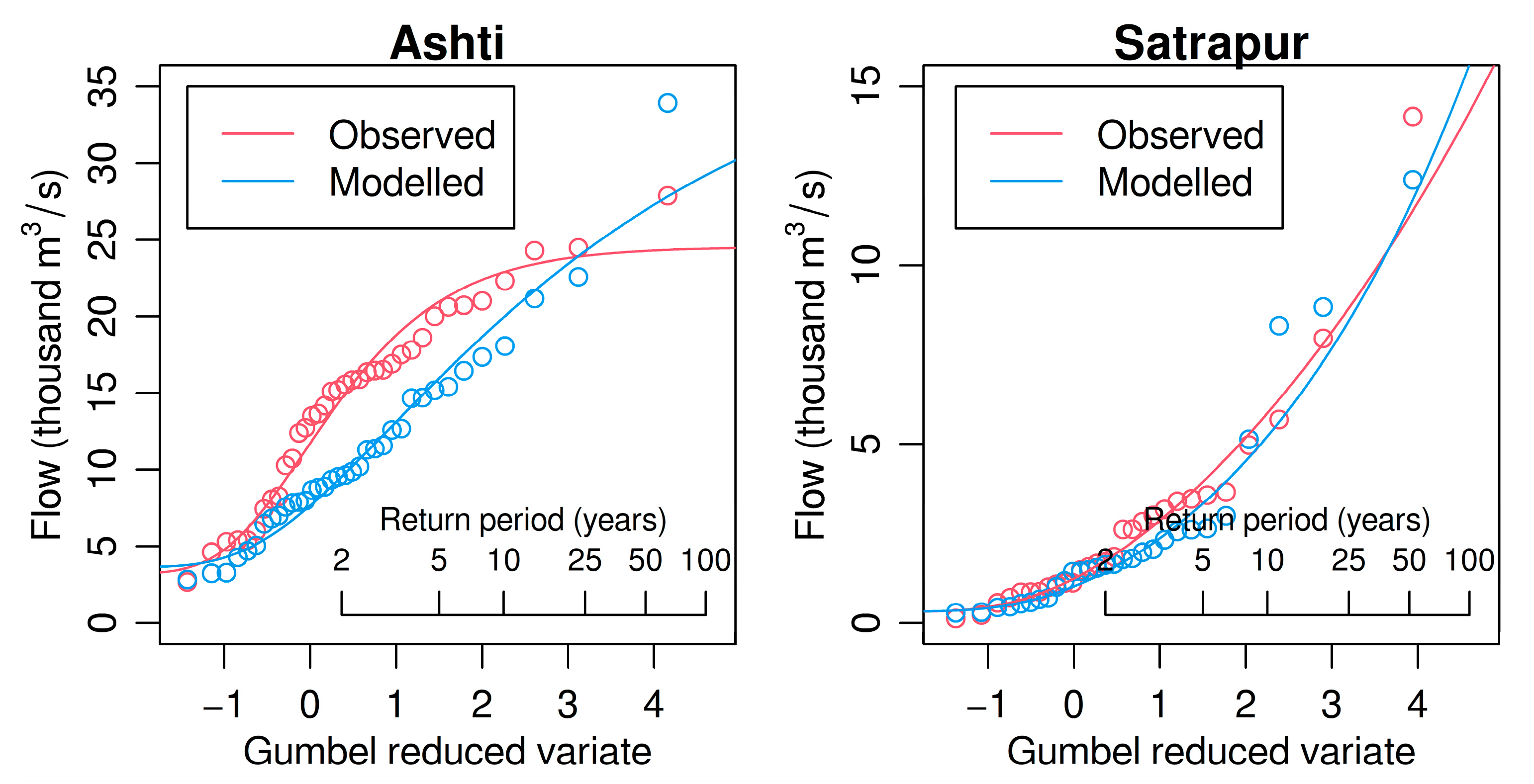
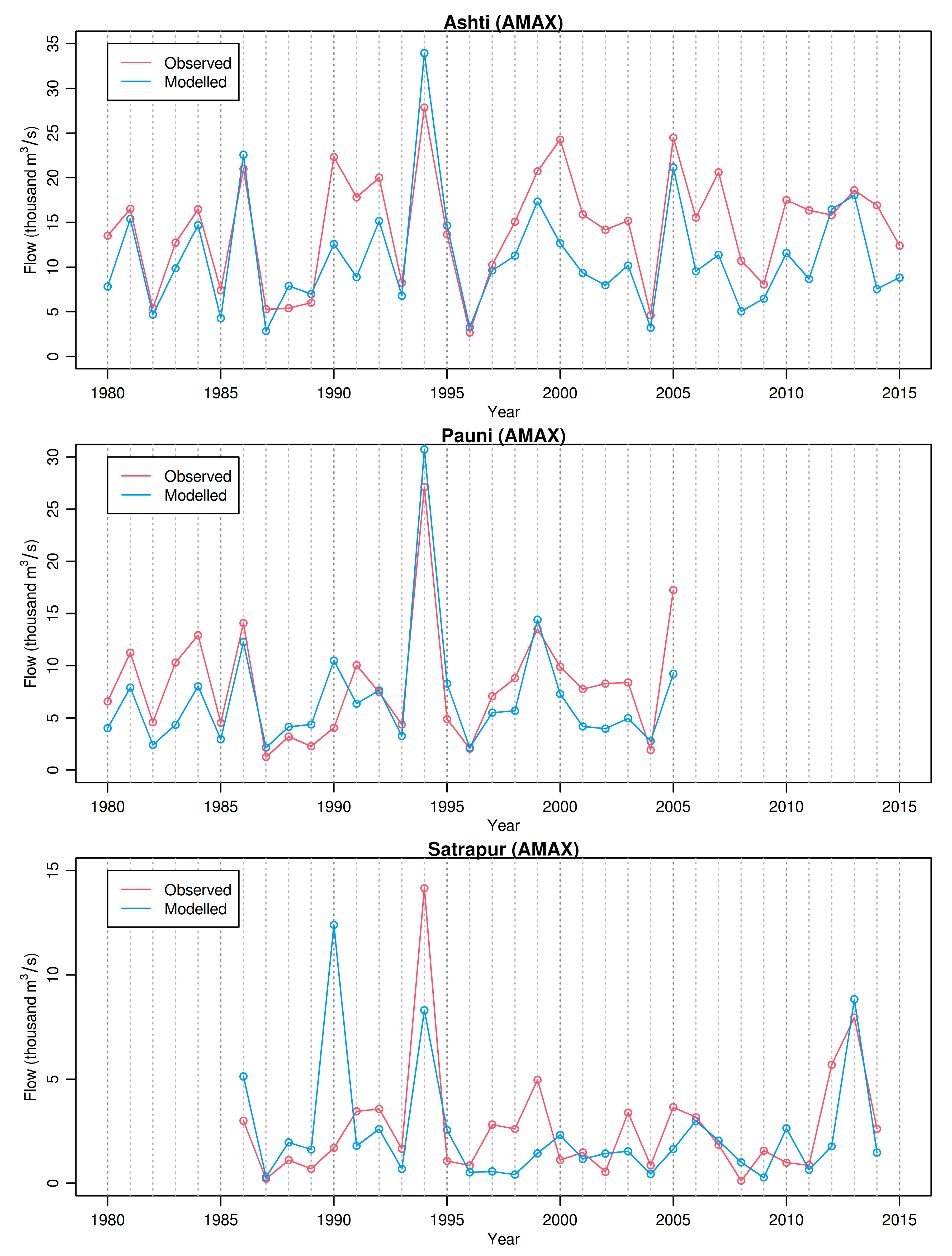
Figure 10 shows the flood frequency curves for Ashti and Satrapur derived through semi-lumped modeling. Pauni is not shown but is midway between Ashti and Satrapur. Despite its very strong KGE’ value, the modeled and observed FFC at Ashti differ. Conversely, the modeled and observed FFC at Satrapur are similar, despite the lower KGE’. Figure 11 shows that the strong performance of the FFC at Satrapur partly arose from the fact that the fit of the FFC was not forced by trying to match observed and modeled AMAX in a given year, unlike the KGE’, which looks at the ordered time-series.

4. Conclusions

In this study, we attempted to produce a method for flood frequency estimation in the Wainganga basin to act as an alternative to statistical analysis that has the potential to be applied at ungauged sites, and in catchments larger than those for which existing guidance [5] is recommended. We did this through continuous simulation modeling, using rainfall and evapotranspiration records as inputs to catchment models. Catchments were modeled in a variety of lumped and semi-lumped configurations, using gauged flows to calibrate and test the models. The models used were the PDM for lumped catchments and sub-catchments, and the kinematic wave for channel routing of flow from upstream lumped catchments to the basin outlet during semi-lumped modeling. The Generalized Pareto distribution was chosen through a Hosking–Wallis approach as the most appropriate distribution for the region, using a wider set of catchments from the surrounding area.
Performance was variable, but was best for the two most downstream catchments, at the Ashti and Pauni gauging stations. This held true for all variants of modeling, suggesting that the exact setup of the catchment model was not one of the most important factors in achieving a close match between modeled and observed runoff. Semi-lumped modeling was found to offer similar performance to lumped modeling, despite the sub-optimality of assigning the same parameter values to all sub-catchments. Semi-distributed modeling with regionalization of parameter values is potentially valuable for future work but could not be tested here due to the limited number of gauges available (nine).
The objective of this study was to improve estimation of annual maximum river flows so that they could be used to estimate extreme flood magnitudes from which flood frequency curves could be developed for the purpose of estimating long return period flood magnitudes. Model calibration in most of this study focused on maximizing KGE’ over the whole range of flows, of which the AMAX value is just one of every 365 or 366 points. While calibration using KGE’ attempts to match the variability of modeled flows to that observed, any under-representation of flow variability is likely to affect the most extreme flows first. An alternative calibration procedure maximizing KGE’ exclusively on annual maxima was tested, as the AMAX are usually the only flows of interest in extreme-event flood frequency analysis. This calibration procedure was not found to improve or impair the model’s predictive performance relative to conventional calibration at the Ashti gauging station in a split-sample test where the final 10 years of flow were not used in calibration. Calibration to AMAX could therefore be used at sites where only an AMAX record is reliable, or the AMAX record is of higher quality than the full river flow time-series, such as stations that only record during the monsoon season. However, any model calibrated in this way should be used only for estimating AMAX flows.
In the study area, large amounts of unquantified artificial influence on flows limited the performance that could be achieved. The scale of artificial influence, particularly from dams, was not constant over the modeling period. This could not be accounted for in the hydrological model as the parameters were static for each model run. While it is possible for the model parameters to change over time (by expressing each parameter value as an equation that includes time since start), there is uncertainty around the exact form of the relationship between any parameter value and time, and whether an apparent trend in time is more accurately represented as a trend in a different covariate that contains a time-varying component (such as a rainfall or wetness index).
Performance is also limited by the accuracy of the data used throughout the study. In particular, there is no clear documentation on how the flow observations, which were used to calibrate the model, were made. It also appears that elevation was not considered during production of the gridded rainfall data that were used to drive the model, implying a bias towards rainfall underestimation at higher altitudes. This may be the reason for poorer performance in matching annual maximum flows in upland headwaters. Improved performance might be achieved by bias correcting the gridded data against high-altitude point gauged data, or by adjusting gridded values to account for elevation.

Author Contributions

Conceptualization, G.V., A.G. and E.S.; methodology, G.V. and A.G.; software, G.V. and A.G.; validation, G.V. and A.G.; formal analysis, G.V. and A.G.; investigation, G.V. and A.G.; resources, E.S.; data curation, G.V., A.G. and E.S.; writing—original draft preparation, G.V., A.G. and E.S.; writing—review and editing, G.V., A.G. and E.S.; visualization, G.V. and A.G.; supervision, E.S.; project administration, E.S.; funding acquisition, E.S. All authors have read and agreed to the published version of the manuscript.

Funding

This research was supported by the UKCEH SUNRISE programme, a National Capability project funded by the Natural Environment Research Council (NERC). The APC was funded by UKCEH’s UK Research and Innovation (UKRI) Open Access Block Grant (OABG).

Data Availability Statement

Rainfall and river flow data were supplied by the Indian Meteorological Department and the Indian Central Water Commission. They are available online at https://www.imdpune.gov.in/Clim_Pred_LRF_New/Grided_Data_Download.html (accessed on 9 August 2022) and https://indiawris.gov.in (accessed on 9 August 2022), respectively.

Acknowledgments

The authors would like to thank Arpita Mondal and Chingka Kalai for their advice, and John Wallbank and two anonymous reviewers for reviewing earlier drafts of this manuscript.

Conflicts of Interest

The authors declare no conflict of interest.

References

  1. Times of India. Mumbai Rains: Misery All Around, BMC Says the Situation Is ‘Exceptional’. Available online: https://timesofindia.indiatimes.com/city/mumbai/mumbai-rains-misery-all-around-bmc-says-the-situation-is-exceptional/articleshow/60284534.cms (accessed on 16 July 2021).
  2. Times of India. Sabarmati Sinks Parts of Ahmedabad. Available online: https://timesofindia.indiatimes.com/india/sabarmati-sinks-parts-of-ahmedabad/articleshow/48289938.cms (accessed on 7 June 2022).
  3. World Meteorological Organization. South Asia Flash Flood Guidance System Launched. Available online: https://public.wmo.int/en/media/news/south-asia-flash-flood-guidance-system-launched (accessed on 21 June 2022).
  4. Yadav, A.B.P.; Raja, B.S.K.A.; Saxena, C.R.; Bharwani, D.H.; Das, E.A.K.; Giri, F.R.K.; Manik, G.S.K.; Yadav, H.D. Recent Advances in Pluvial Flash Flood Forecasting of India. In Innovative Trends in Hydrological and Environmental Systems; Dikshit, A.K., Narasimhan, B., Kumar, B., Patel, A.K., Eds.; Springer: Singapore, 2022; pp. 605–643. [Google Scholar]
  5. Central Water Commission. Flood Estimation Report for Lower Godavari Subzone 3(f); Central Water Commission: New Delhi, India, 1980. [Google Scholar]
  6. Central Water Commission. Flood Estimation Report for Upper Godavari Subzone 3(e); Central Water Commission: New Delhi, India, 1986. [Google Scholar]
  7. Central Water Commission. Flood Estimation Report for Krishna and Pennar Subzone 3(h); Central Water Commission: New Delhi, India, 2000. [Google Scholar]
  8. Bhunya, P.K.; Panigrahy, N.; Kumar, R.; Berndtsson, R. Development of a Regional Non-Dimensional Return Period Flood Model. Water Resour. Res. 2010, 24, 1425–1439. [Google Scholar] [CrossRef]
  9. Garde, R.J.; Kothyari, U.C. Flood Estimation in Indian Catchments. J. Hydrol. 1990, 113, 135–146. [Google Scholar] [CrossRef]
  10. Swamee, P.K.; Ojha, C.S.P.; Abbas, A. Mean Annual Flood Estimation. J. Water Resour. Plan. Manag. 1995, 121, 403–407. [Google Scholar] [CrossRef]
  11. Singh, K.K.; Pal, M.; Singh, V.P. Estimation of Mean Annual Flood in Indian Catchments Using Backpropagation Neural Network and M5 Model Tree. Water Resour. Manag. 2010, 24, 2007–2019. [Google Scholar] [CrossRef]
  12. Formetta, G.; Prosdocimi, I.; Stewart, E.; Bell, V. Estimating the index flood with continuous hydrological models: An application in Great Britain. Hydrol. Res. 2017, 49, 123–133. [Google Scholar] [CrossRef]
  13. Ministry of Water Resources. Krishna Basin Report Ver. 2; Government of India: New Delhi, India, 2014. [Google Scholar]
  14. South Asia Network on Dams Rivers and People (SANDRP). Wainganga River: Threatened Lifeline of Vidarbha’s Forests. Available online: https://sandrp.in/2017/04/14/wainganga-river-threatened-lifeline-of-vidarbhas-forests (accessed on 30 July 2021).
  15. Central Water Commission (CWC). National Register of Large Dams; Central Water Commission: New Delhi, India, 2019. [Google Scholar]
  16. WAPCOS. PFR Studies of Wainganga H.E. Project; WAPCOS: New Delhi, India, undated.
  17. National Water Informatics Centre. India-WRIS (India Water Resources Information System). Available online: https://indiawris.gov.in (accessed on 7 June 2022).
  18. Lehner, B.; Grill, G. Global river hydrography and network routing: Baseline data and new approaches to study the world’s large river systems. Hydrol. Process. 2013, 27, 2171–2186. [Google Scholar] [CrossRef]
  19. Lehner, B.; Verdin, K.; Jarvis, A. New global hydrography derived from spaceborne elevation data. EOS Trans. Am. Geophys. Union 2008, 89, 93–94. [Google Scholar] [CrossRef]
  20. Lehner, B. HydroSHEDS Technical Documentation (version 1.4); World Wildlife Fund US: Washington, DC, USA, 2022. [Google Scholar]
  21. Messager, M.L.; Lehner, B.; Grill, G.; Nedeva, I.; Schmitt, O. Estimating the Volume and Age of Water Stored in Global Lakes Using a Geo-Statistical Approach. Nat. Commun. 2016, 7, 13603. [Google Scholar] [CrossRef]
  22. Slater, J.A.; Garvey, G.; Johnston, C.; Haase, J.; Heady, B.; Kroenung, G.; Little, J. The SRTM data “finishing” process and products. Photogramm. Eng. Remote Sens. 2006, 72, 237–247. [Google Scholar] [CrossRef]
  23. Lehner, B.; Liermann, C.R.; Revenga, C.; Vörösmarty, C.; Fekete, B.; Crouzet, P.; Döll, P.; Endejan, M.; Frenken, K.; Magome, J.; et al. Global Reservoir and Dam Database, Version 1 (GRanDv1): Dams, Revision 01; NASA Socioeconomic Data and Applications Center (SEDAC): Palisades, NY, USA, 2011. [Google Scholar]
  24. Lehner, B.; Liermann, C.R.; Revenga, C.; Vörösmarty, C.; Fekete, B.; Crouzet, P.; Döll, P.; Endejan, M.; Frenken, K.; Magome, J.; et al. High-Resolution Mapping of the World’s Reservoirs and Dams for Sustainable River-Flow Management. Front. Ecol. Environ. 2011, 9, 494–502. [Google Scholar] [CrossRef] [Green Version]
  25. Pai, D.S.; Sridhar, L.; Rajeevan, M.; Sreejith, O.P.; Satbhai, N.S.; Mukhopadyay, B. Development of a new high spatial resolution (0.25° × 0.25°) Long Period (1901–2010) daily gridded rainfall data set over India and its comparison with existing data sets over the region. Mausam 2014, 65, 1–18. [Google Scholar] [CrossRef]
  26. Funk, C.; Peterson, P.; Landsfeld, M.; Pedreros, D.; Verdin, J.; Shukla, S.; Husak, G.; Rowland, J.; Harrison, L.; Hoell, A.; et al. The climate hazards infrared precipitation with stations—A new environmental record for monitoring extremes. Sci. Data 2015, 2, 150066. [Google Scholar] [CrossRef] [PubMed]
  27. Miralles, D.G.; Holmes, T.R.H.; de Jeu, R.A.M.; Gash, J.H.; Meesters, A.G.C.A.; Dolman, A.J. Global land-surface evaporation estimated from satellite-based observations. Hydrol. Earth Syst. Sci. 2011, 15, 453–469. [Google Scholar] [CrossRef]
  28. Martens, B.; Miralles, D.G.; Lievens, H.; van der Schalie, R.; de Jeu, R.A.M.; Fernández-Prieto, D.; Beck, H.E.; Dorigo, W.A.; Verhoest, N.E.C. GLEAM v3: Satellite-based land evaporation and root-zone soil moisture. Geosci. Model Dev. 2017, 10, 1903–1925. [Google Scholar] [CrossRef]
  29. Fischer, G.; Nachtergaele, F.O.; Prieler, S.; Teixeira, E.; Toth, G.; van Velthuizen, H.; Verelst, L.; Wiberg, D. Global Agro-Ecological Zones Assessment for Agriculture (GAEZ 2008); IIASA: Laxenburg, Austria; FAO: Rome, Italy, 2012. [Google Scholar]
  30. Bayliss, A. Catchment Descriptors (Flood Estimation Handbook Volume 5); Institute of Hydrology: Wallingford, UK, 1999. [Google Scholar]
  31. Hosking, J.R.M.; Wallis, J.R. Regional Frequency Analysis: An Approach Based on L-Moments; Cambridge University Press: Cambridge, UK, 1997. [Google Scholar]
  32. Kjeldsen, T.R.; Jones, D.A.; Bayliss, A.C. Improving the FEH Statistical Procedures for Flood Frequency Estimation; Environment Agency: Bristol, UK, 2008. [Google Scholar]
  33. R Core Team. R: A Language and Environment for Statistical Computing; R Foundation for Statistical Computing: Vienna, Austria, 2016. [Google Scholar]
  34. Hosking, J.R.M. Regional Frequency Analysis Using L-Moments (R package). Available online: https://cran.r-project.org/package=lmomRFA (accessed on 15 July 2022).
  35. Moore, R.J. The PDM rainfall-runoff model. Hydrol. Earth Syst. Sci. 2007, 11, 483–499. [Google Scholar] [CrossRef]
  36. Kling, H.; Fuchs, M.; Paulin, M. Runoff conditions in the upper Danube basin under an ensemble of climate change scenarios. J. Hydrol. 2012, 424-425, 264–277. [Google Scholar] [CrossRef]
  37. Duan, Q.; Sorooshian, S.; Gupta, V. Effective and efficient global optimization for conceptual rainfall-runoff models. Water Resour. Res. 1992, 28, 1015–1031. [Google Scholar] [CrossRef]
  38. Duan, Q.; Sorooshian, S.; Gupta, V. Optimal use of the SCE-UA global optimization method for calibrating watershed models. J. Hydrol. 1994, 158, 265–284. [Google Scholar] [CrossRef]
  39. Drissia, T.K.; Jothiprakash, V.; Anitha, A.B. Flood frequency analysis using L-moments: A comparison between at-site and regional approach. Water Resour. Manag. 2019, 33, 1013–1037. [Google Scholar] [CrossRef]
  40. Guru, N.; Jha, R. Flood frequency analysis of Tel basin of Mahanadi river system, India using annual maximum and POT flood data. Aquat. Procedia 2015, 4, 427–434. [Google Scholar] [CrossRef]
  41. Swetapadma, S.; Ojha, C.S.P. Selection of a basin-scale model for flood frequency analysis in Mahanadi river basin, India. Nat. Hazards 2020, 102, 519–552. [Google Scholar] [CrossRef]
  42. Kumar, R.; Goel, N.K.; Chatterjee, C.; Nayak, P.C. Regional flood frequency analysis using soft computing techniques. Water Resour. Manag. 2015, 29, 1965–1978. [Google Scholar] [CrossRef]
  43. Kumar, R.; Chatterjee, C.; Kumar, S.; Lohani, A.K.; Singh, R.D. Development of regional flood frequency relationships using L-moments for Middle Ganga Plains subzone 1(f) of India. Water Resour. Manag. 2003, 17, 243–257. [Google Scholar] [CrossRef]
  44. Grimaldi, S.; Nardi, F.; Piscopia, R.; Petroselli, A.; Apollonio, C. Continuous hydrologic modelling for design simulation in small and ungauged basins: A step forward and some tests for its practical use. J. Hydrol. 2021, 595, 125664. [Google Scholar] [CrossRef]
  45. Ball, J.E. Modelling Accuracy for Reliable Urban Design Flood Estimation. In Proceedings of the HWRS 2021: Digital Water: Hydrology and Water Resources Symposium, Virtual Symposium, 31 August–1 September 2021; Engineers Australia: Barton, Australia, 2021; pp. 35–47. [Google Scholar]
  46. Hossain, S.; Hewa, G.A.; Wella-Hewage, S. A Comparison of Continuous and Event-Based Rainfall-Runoff (RR) Modelling Using EPA-SWMM. Water 2019, 11, 611. [Google Scholar] [CrossRef]
  47. Nair, S.C.; Mirajkar, A.B. Integrated watershed development plan for a sub-basin, central India. Water Supply 2022, 22, 3342–3351. [Google Scholar] [CrossRef]
  48. Criss, R.E.; Winston, W.E. Do Nash values have value? Discussion and alternate proposals. Hydrol. Process. 2008, 22, 2723–2725. [Google Scholar] [CrossRef]
  49. de Lavenne, A.; Thirel, G.; Andréassian, V.; Perrin, C.; Ramos, M.-H. Spatial variability of the parameters of a semi-distributed hydrological model. Proc. Int. Assoc. Hydrol. Sci. 2016, 373, 87–94. [Google Scholar] [CrossRef]
  50. de Lavenne, A.; Andréassian, V.; Thirel, G.; Ramos, M.-H.; Perrin, C. A regularization approach to improve the sequential calibration of a semi-distributed hydrological model. Water Resour. Res. 2019, 55, 8821–8839. [Google Scholar] [CrossRef]
  51. Pradhan, C.; Chembolu, V.; Bharti, R.; Dutta, S. Regulated rivers in India: Research progress and future directions. ISH J. Hydraul. Eng. 2021, in press. [Google Scholar] [CrossRef]
  52. Mubialiwo, A.; Abebe, A.; Onyutha, C. Performance of rainfall-runoff models in reproducing hydrological extremes: A case of the River Malaba sub-catchment. SN Appl. Sci. 2021, 3, 515. [Google Scholar] [CrossRef]
  53. Soriano, E.; Mediero, L.; Garijo, C. Quantification of Expected Changes in Peak Flow Quantiles in Climate Change by Combining Continuous Hydrological Modelling with the Modified Curve Number Method. Water Resour. Manag. 2020, 34, 4381–4397. [Google Scholar] [CrossRef]
  54. Le Moine, N. Le Bassin Versant de Surface vu Par le Souterrain: Une Voie D’amélioration des Performances et du Réalisme des Modèles Pluie-Débit? Ph.D. Thesis, Université Pierre et Marie Curie, Paris, France, 2008. [Google Scholar]
  55. Lobligeois, F. Mieux Connaître la Distribution Spatiale des Pluies Améliore-t-il la Modélisation des Crues? Diagnostic Sur 181 Bassins Versants Français. Ph.D. Thesis, AgroParisTech, Paris, France, 2014. [Google Scholar]
  56. Pechlivanidis, I.G.; McIntyre, N.R.; Wheater, H.S. Calibration of the semi-distributed PDM rainfall-runoff model in the Upper Lee catchment, UK. J. Hydrol. 2010, 386, 198–209. [Google Scholar] [CrossRef]
  57. Kjeldsen, T.R. Flood Estimation Handbook Supplementary Report No. 1: The Revitalised FSR/FEH Rainfall-Runoff Method; Centre for Ecology & Hydrology: Wallingford, UK, 2007. [Google Scholar]
Figure 1. (a) Map of the Wainganga, Godavari and Krishna basins within central/south mainland India; (b) Close-up of the Wainganga catchment and sub-catchments with named river gauging stations and cities.
Water 14 02887 g001
Figure 2. Study methodological diagram.
Water 14 02887 g002
Figure 3. Hosking–Wallis distribution test results over the Krishna and Godavari basins. Wainganga sub-catchments are outlined in black.
Water 14 02887 g003
Figure 4. Growth curves associated to (left) Wadakbal gauging station on the Sina River, QMED = 581 m3/s, and (right) Pathagudem gauging station on the Indravathi River, QMED = 10,045 m3/s. Gray × symbols indicate ranked gauged AMAX flows at each station.
Water 14 02887 g004
Figure 5. Modeled vs observed QMED, l1 (sample L-mean), l2 (sample L-CV) and t3 (sample L-SKEW) for nine Wainganga station AMAX records.
Water 14 02887 g005
Figure 6. Modeled total flow and slow flow for Pauni, May–December 1994.
Water 14 02887 g006
Figure 7. Observed and modeled flood frequency curves for Ashti and Ramakona.
Water 14 02887 g007
Figure 8. Observed and modeled flood frequency curves for Ashti and Ramakona (PDM optimized for AMAX only).
Water 14 02887 g008
Figure 9. Observed (red line) and modeled AMAX series for Ashti when PDM is optimized to match AMAX from 1983–2006 inclusive (blue line) and optimized to match the whole flow regime from 1983–2006 inclusive (yellow line).
Water 14 02887 g009
Figure 10. Observed and modeled flood frequency curves for Ashti and Satrapur (semi-lumped modeling).
Water 14 02887 g010
Figure 11. Observed and modeled AMAX series for Ashti, Pauni and Satrapur for semi-lumped modeling.
Water 14 02887 g011
Table 1. Sub-catchments of the Wainganga considered in this study.
NameStart YearEnd YearArea (km2)DPLBAR (km)DPSBAR (m/km)CULT
(-)
URB
(-)
FOR
(-)
Ashti1965201651579339.033.40.4700.0510.394
Kumhari198620178417118.038.90.4610.0400.380
Pauni1964201636023217.036.90.4990.0570.349
Rajegaon19852017539369.748.70.3660.0430.527
Rajoli19862015267554.519.20.4890.0330.405
Ramakona19862017248882.354.90.5380.0410.295
Salebardi19852014176844.030.40.4390.0370.469
Satrapur1984201511161142.044.50.5190.0590.305
Wairagarh19922015175542.541.10.2330.0300.704
Note(s): DPLBAR = mean drainage path length, DPSBAR = mean drainage path slope, CULT = total cultivated land fraction, URB = built-up land fraction, FOR = forested land fraction.
Table 2. Number of stations at which each distribution is acceptable (|ZDIST| < 1.64) and chosen (|ZDIST| = min(|ZDIST|)) to describe the annual maximum (AMAX) series.
DistributionGLOGEVGNOPE3GPA
Accepted67919510192
Chosen1717122947
Table 3. Performance metrics (lumped sub-catchment modeling).
CatchmentKGErγβNSE
Ashti0.8800.8810.9981.0070.760
Kumhari0.5120.5130.9651.0010.057
Pauni0.8580.8581.0071.0080.712
Rajegaon0.6690.6700.9751.0060.352
Rajoli0.5480.5580.9051.0100.183
Ramakona0.3330.3350.9520.993−0.262
Salebardi0.6480.6540.9371.0030.346
Satrapur0.5730.5750.9640.9810.194
Wairagarh0.4860.4880.9711.032−0.026
Table 4. Performance metrics (lumped sub-catchment modeling, optimizing performance on AMAX only).
CatchmentKGErγβNSE
Ashti0.6470.8600.9221.3150.602
Kumhari0.3560.3991.0300.7690.001
Pauni0.6670.7441.1320.8330.510
Rajegaon0.3530.5610.8551.452−0.163
Rajoli−0.5160.5610.6122.398−0.659
Ramakona0.1600.2990.9931.462−1.250
Salebardi0.3970.6370.7531.4130.209
Satrapur0.3500.5171.3730.775−0.033
Wairagarh0.4370.4410.9490.963−0.030
Table 5. Performance metrics (lumped sub-catchment modeling, single parameter set).
CatchmentKGErγβNSE
Ashti0.6580.7631.0490.7580.574
Kumhari0.3240.4930.9030.5630.230
Pauni0.7380.7901.0600.8540.608
Rajegaon0.5140.6650.8240.6940.427
Rajoli0.0010.6120.7031.871−0.179
Ramakona0.2930.3490.7420.9000.020
Salebardi0.5030.6680.6640.8450.433
Satrapur0.2910.5050.8031.468−0.211
Wairagarh0.4160.4720.8720.7840.172
Table 6. Performance metrics (semi-lumped modeling, single parameter set).
CatchmentKGErγβNSEKGE’’
Ashti0.8670.8680.9801.0030.7410.860
Pauni0.8740.8740.9991.0000.7490.844
Satrapur0.5750.5790.9550.9700.2140.518
Publisher’s Note: MDPI stays neutral with regard to jurisdictional claims in published maps and institutional affiliations.