Article

Assessment of Seasonal Surface Runoff under Climate and Land Use Change Scenarios for a Small Forested Watershed: Upper Tarlung Watershed (Romania)

by
Mirabela Marin
1,2,
Ioan Clinciu
2,
Nicu Constantin Tudose
1,*,
Cezar Ungurean
1,
Alin Lucian Mihalache
1,2,
Nicoleta Emilia Martoiu
1 and
Oana Nicoleta Tudose
1
1
Watershed Management Department, National Institute for Research and Development in Forestry “Marin Dracea”, 500040 Brasov, Romania
2
Faculty of Silviculture and Forest Engineering, Transilvania University of Brasov, 500036 Brașov, Romania
*
Author to whom correspondence should be addressed.
Water 2022, 14(18), 2860; https://doi.org/10.3390/w14182860
Submission received: 25 July 2022 / Revised: 8 September 2022 / Accepted: 9 September 2022 / Published: 13 September 2022
(This article belongs to the Section Hydrology)

Abstract

:
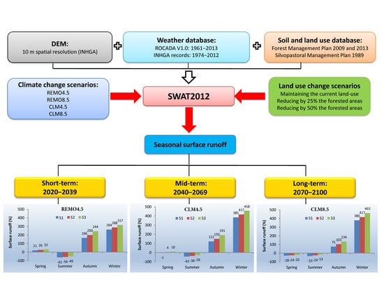
This study aims to evaluate the potential impact of climate and land use change on seasonal dynamics of surface runoff within the Upper Tarlung watershed of 71.62 km2. Using the Soil and Water Assessment Tool (SWAT), we simulated the surface runoff under the projections from four global and regional combination models for two representative concentration pathways (RCP4.5 and RCP8.5) and three land use change scenarios. In addition, short (2020–2039), mid (2040–2069), and long-term model simulations (2070–2100) were analyzed compared with a ten-year baseline period (1979–1988). Ensemble SWAT outputs showed that, in spring, surface runoff could decrease by up to 28% or increase by up to 86%, in summer can decrease by up to 69%, while in autumn and winter, increases of approximately two to five times fold are expected. The decreasing tendency is more pronounced under climate conditions, while the sharpest increases are estimated in the comprehensive scenario of climate and land use change by 50%. Those results serve as a support for local water, forest, and land managers in anticipating possible threats and conceiving adaptive strategies to manage the studied watershed efficiently.

Graphical Abstract

1. Introduction

Climate change generates important increases in global surface temperatures and shifts in precipitation patterns that represent a significant concern for policy and decision-makers. The latest projections of the IPCC include five new scenarios (SSP1-1.9, SSP1-2.6, SSP2-4.5, SSP3-7.0, and SSP5-8.5) that cover a wide range of socio-economic, technological, and political developments and are based on the Shared Socioeconomic Pathways (SSPs) [1]. According to these new narratives, 2021–2100, compared to the 1850–1900 period is very likely to see increases in air temperature between 1.0–5.7 °C. The precipitation regime will vary across regions, while heavy precipitation, heatwaves, and warm spell events will become more frequent and intense [1,2]. These changes will trigger severe consequences for water resources [3,4,5,6], forests [7,8], and human wellbeing [9]. Water is a key component for ensuring the sustainable development of society [10,11] and is directly mentioned in the SDG 6 ‘Clean water and sanitation’ and tangentially addressed in the SDG3 ‘Ensure healthy lives and promote well-being for all at all ages’, SDG11 ‘Make cities and human settlements inclusive, safe, resilient, and sustainable’, SDG12 ‘Ensure sustainable consumption and production patterns’, and SDG15 ‘Protect, restore, and promote sustainable use of terrestrial ecosystems, sustainably manage forests, combat desertification, and halt and reverse land degradation and halt biodiversity loss’ of the Agenda 2030 for the Sustainable Development of the United Nations [12]. To make advances in sustainability achievement and to strengthen society and environmental resilience as drivers of change, many European legislations were conceived to guide policy and decision-makers toward sustainable management of natural resources (e.g., the European Green Deal (https://ec.europa.eu/environment/strategy/biodiversity-strategy-2030_en; Accessed on 30 June 2022), New EU Forest Strategy for 2030 (https://www.eesc.europa.eu/en/our-work/opinions-information-reports/opinions/new-eu-forest-strategy-2030; Accessed on 30 June 2022), EU Soil Strategy for 2030 (https://eur-lex.europa.eu/legal-content/EN/TXT/PDF/?uri=CELEX:52021DC0699&from=EN; Accessed on 30 June 2022), EU Biodiversity Strategy for 2030 (https://ec.europa.eu/environment/strategy/biodiversity-strategy-2030_en; Accessed on 30 June 2022), and EU Action Plan: ‘Towards Zero Pollution for Air, Water and Soil’ (https://eur-lex.europa.eu/resource.html?uri=cellar:a1c34a56-b314-11eb-8aca-01aa75ed71a1.0001.02/DOC_1&format=PDF; Accessed on 30 June 2022). Unfortunately, the COVID-19 pandemic has drawn back the progress recorded during 2015–2018 in achieving the SDG targets and indicators until unprecedented reversals for the end of 2021, and more efforts will be needed to meet the ambitions of the 2030 agenda [13].
Water is the central pillar of the circular development of society [11,14]. There is evidence that emphasizes climate and land use change as the main driving forces in influencing the water resources availability [15,16,17,18]. Numerous publications have tackled water resource dynamics under current and future challenges and have shown a decreased tendency of water resources worldwide [19,20,21,22,23]. For instance, Guzha et al.’s [19] evaluations of the impact of land use and land cover on surface runoff have found that forest reductions lead to increases by up to 90% of surface runoff, while low flows can decrease up to 46%. According to Ouyang et al. [20], surface runoff can decrease by approximately 29%, while at the seasonal level, surface runoff can be reduced by up to 40%, and significant variations of this parameter are expected during winter as a response to forest change.
Moreover, Sabbaghi et al. [21] revealed that climate change would lead to 4.3% and 8.1% decreases in discharges in 2040 and 2070, respectively. The authors also emphasized the importance of proper water allocation within river basins to avoid climate change negative effects. In this context, Gemechu et al. [23] reported decreases by up to 8.9% of water yield for the 2030 and 2080 periods considering the RCP4.5 and 8.5 scenarios. The authors also estimated important monthly changes when water yield can decrease to 27% and 32% in RCP4.5 and 8.5, respectively, and increase by up to 28% in RCP4.5. After applying the SWAT model to evaluate the climate change impacts on runoff, Wu et al. [24] estimated a reduction of 54.1% of surface runoff, while Wang et al. [25] reported an increase of 11.87% due to land use change. Increases in surface runoff due to land use change are also reported by Chilagane et al. [26] who estimated that forest reduction contributed to surface runoff increases on an annual basis, while at the seasonal level, there were expected decreases in the dry season (July–October) until 2040, thus emphasizing the need of appropriate conservations strategies.
According to studies in [22,27], the prediction of water resource variations under different challenges using different modeling tools is mandatory for short- and long-term adaptive planning. Thereby, hydrological information is fundamental to watershed behavior under growing pressures, thus avoiding uneven water allocation between socio-economic and environmental users [28]. At the same time, water resources should be accurately evaluated to ensure their future sustainability [29].
From this perspective, a comprehensive understanding of watershed responses under various scenarios is imperative [9]. Such an achievement is tapped through hydrological modeling, which is recognized as a valuable approach to understand and assess the effects of different forcings (e.g., climate, land use) on hydrological processes within watersheds [30]. Hydrological models could predict the possible impacts of climate and land use changes [31]. Estimating in a more realistic way the effects of those changes will allow stakeholders to adopt proactive planning for sustainable watershed management [32].
Existing hydrological models facilitate the evaluation of different impacts on hydrological processes in different-sized watersheds and over variable periods. In this context, the Soil and Water Assessment Tool (SWAT) hydrological model is widely applied and very efficient for exploring the long-term impacts of a wide variety of forcings, including climate and land use change on hydrological processes within watersheds [5,33]. SWAT simulates many hydrological processes, such as evapotranspiration, percolation, canopy storage, lateral and groundwater flow, surface runoff, and so forth. SWAT model-wide use is very common in the discipline since it is an open-source software with a predefined database that can be easily customized by the user [33]. This integrated model is appropriate even in an ungauged watershed, where discharge data are missing [34,35,36]. Compared to other models, such as Mike-SHE (European Hydrological System Model) or GSSHA (Gridded Surface/Subsurface Hydrologic Analysis) for example, SWAT requests few input parameters that can be easily generated by the model if there are missing or discontinuous data [37].
For sustainable management of these particular watersheds, the water’s spatial and temporal dynamics are essential [38], particularly in the context of the combined effect of increased temperature, changed patterns of precipitations, and increased frequency of extreme events (floods, droughts, heatwaves) occurrence in southeastern Europe, including Romania [3,39,40]. The combined effect of increased temperatures and the opposite trend of precipitation may cause perilous natural hazards, especially in mountainous regions [41], which are known to be areas sensitive to climate change [42]. Additionally, the changes in land use categories can modify runoff processes, particularly in small watersheds [43,44]. Considering these issues and the consensus that in mountainous areas, the ongoing changes in climate parameters trigger additional pressures on ecosystem management [6,45], special attention should be devoted to mountainous, forested watersheds that accomplish the water supply function [38,46]. There is evidence that surface runoff in a forested watershed is more impacted by changes in land use categories than climate change [47]. As Ouyang et al. [20] claims, most studies have considered evaluating the dynamics of hydrological processes on an annual level, while the seasonal projections have often been overlooked. From this point of view, there is a need to fill this gap by assessing seasonal surface runoff, particularly in small mountainous, mainly forested watersheds.
Therefore, this study aims to provide information about seasonal surface runoff projected for the 2020–2100 period under comprehensive climate and land use change scenarios. In this respect, two specific objectives were established: (i) to quantify future patterns of temperature and precipitation under four local climate change scenarios, and (ii) to evaluate future dynamics of seasonal surface runoff under compounded scenarios of climate and land use change applied for the 2020–2100 period. By addressing those objectives, our research will provide a scientific basis to guide stakeholders and decision-makers towards more informed decisions and sustainable watershed management. First, we start with a brief presentation of the study area and methodology used in Section 2. Second, in Section 3 and Section 4, we evaluate future projections of temperature and precipitation, and we analyze and discuss the impact of various scenarios of climate and land use change on seasonal surface runoff until 2100. Finally, a wide range of conclusions will be drawn at the end of Section 4.

2. Materials and Methods

2.1. Study Area Description

The Tarlung river basin is situated in the central part of Romania, between 45′30′56″ N and 25°48′13″ E [48]. Covering a total area of 184 km2, it is an ungauged river basin responsible for more than 90% of the water demand of the Brasov metropolitan area. From the entire Tarlung river basin area, we chose the upper sector to be addressed in this study (Figure 1). The Upper Tarlung watershed covers 71.6 km2 and its elevation ranges between 874 and 1842 m a.s.l. The watershed has a length of the hydrographic network of 216.49 km and the main stream length of 14.95 km [49]. The average slope within the Tarlung watershed is 37%, and the main riverbed slope is 6%.
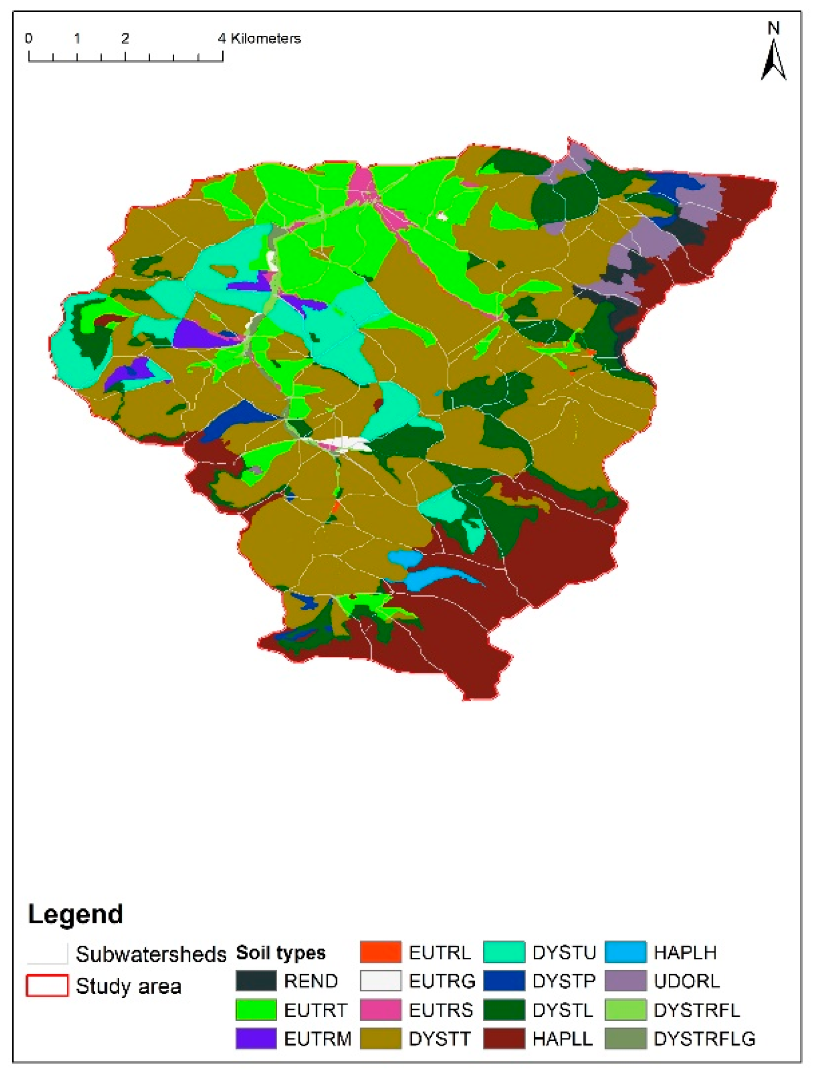
The land within the Upper Tarlung watershed comprises 50% deciduous forests, 30% evergreen forests, 19% pastures, and 1% is covered by pastures with scattered trees, meadows, water bodies, rocky lands, public roads, and built-up area (Figure 2). The main soil types within the watershed are Dystric Cambosols, Prepodzols, and Eutric Cambisoils which account for 60%, 16%, and 15%, respectively (Figure 3).

2.2. Methodology Description

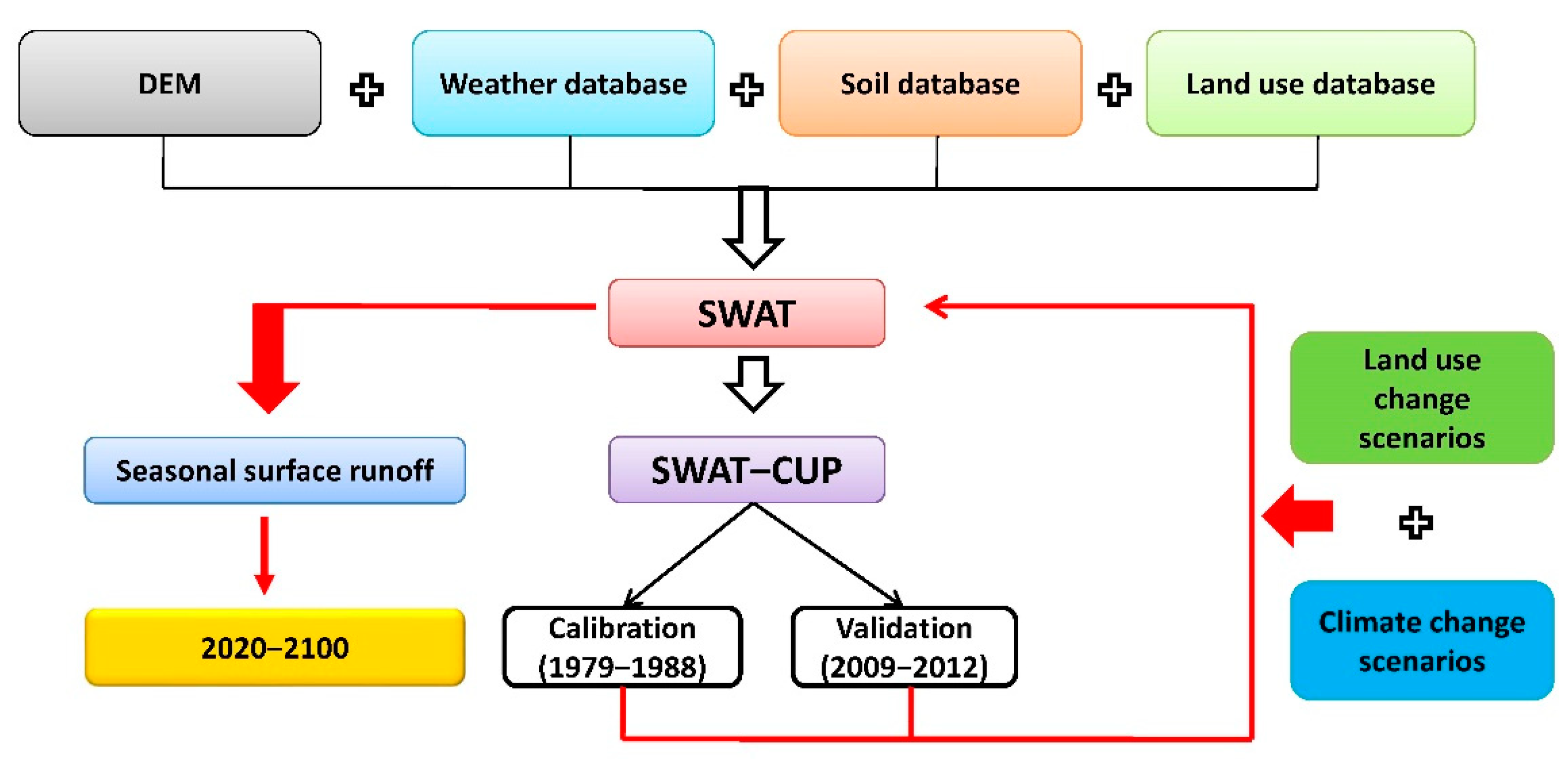
This study uses the SWAT2012 hydrological model and ArcGIS10.3 interface to simulate surface runoff. Developed by the USDA Agricultural Research Service (ARS) to support water managers in investigating an extensive array of problems and continuously improving since 1990, SWAT is continuous-time and semi-distributed which allows daily, monthly, or yearly simulations [36]. SWAT uses an ArcSWAT interface of GIS software for graphical and vectorial edits of the entire watershed that is divided into subwatersheds and subsequently into Hydrologic Response Units (HRU) based on uniform land use, soil types, and slope class [34,36]. In addition, the model requests certain inputs of spatial data, namely: the digital elevation model (DEM), weather database, land use database, and soil database (Figure 4).
For this study, we used a DEM with a 10 m spatial resolution provided by the National Institute of Hydrology and Water Management (INHGA) [48,49]. For the weather database, we used two climate datasets from ROCADA V1.0 and INHGA, which are available for the 1961–2013 and 1974–2012 periods [48,49]. The land use database was customized at the local specificity of the studied watershed based on the data collected from the Forest management plan and Forest-pastoral management plan developed by the National Institute of Research and Development in Forestry ‘Marin Dracea’ (INCDS) for the 1989–2013 period [48,49]. The soil database was created using data from the aforementioned management plans and SPAW (Soil-Plant-Atmosphere-Water-Field and Pond Hydrology) software for estimating parameters for which we had no data available (e.g., bulk density–SOL_BD, hydraulic conductivity–SOL_K, and water content–SOL_AWC) [48,49]. Based on the DEM, the stream network was generated, the subwatersheds were delineated (69 subwatersheds), and HRUs were created (1001 HRUs) [49]. A detailed presentation of the SWAT database customization, model setup, calibration, and validation are given in previous work [49].
The three land use change scenarios were hypothetically established based on the assumption that a reduction of less than 20% of forested areas does not show significant changes in the evolution of hydrological processes [50]. Therefore, the shift of land use change categories from forest (FRSD and FRSE) to pasture (PAST) were randomly modified without considering a certain location across the watershed or other characteristics of the compartment level units (e.g., surface, type of tree species) and was stopped once the percentages (25% and 50%) were obtained [51]. The climate change scenarios used in this study cover the 2020–2100 period and were developed based on a combination of two global climate models, ICHEC-EC-EARTH and MPI-ESM-LR, with two regional climate models CCLM4-8-17 and REMO at 0.11° × 0.11° spatial resolution and forced by RCP4.5 and RCP8.5 representative concentration pathways. These climate models were chosen because they show years with drought periods (2–3 years), relevant for water managers to provide a suitable water demand plan (below Q 1 880   m m · Y e a r 1 in historical data). Additionally, these showed a reasonable evolution of the values of Quartile 1 (Q1) along the projection; thus, bias toward very rainy and very dry models was avoided [52]. A detailed presentation of the climate change scenarios development is given in previous work [53]. The adopted scenarios used in the simulation represent a combination of land use and climate change scenarios, as given in Table 1.
The climate change scenarios included rainfall, temperature, solar radiation, wind speed, and relative humidity data that were downscaled and bias corrected at a local level using the Linear Scaling Method [54,55,56]. Each parameter dataset was used to rewrite the weather database to conduct simulations and obtain future projections of surface runoff. The time period considered in performing simulations was 2020–2100, in order to provide information to warning decision-makers regarding future watershed management in the context of future challenges (e.g., climate and land use) so that they can secure a long-term management plan. Moreover, for the 1988–2020 period, in the study area, there were no notable changes in terms of land use. Major changes appeared after 2015, due to the fragmentation of land ownership through various retrocession laws that corroborated with the intensification of extreme weather events and with the demographic development of the area [57]. For comparison, the 1979–1988 period was chosen as a baseline. For this interval, the flow measurements were continuous, and we identified periods with dry, average, and rainy years which represents an essential condition to obtain accurate simulation results [58]. The future changes in surface runoff were appraised at the seasonal level: spring (March, April, May), summer (June, July, August), autumn (September, October, November), and winter (December, January, February).

3. Results

3.1. Model Performance

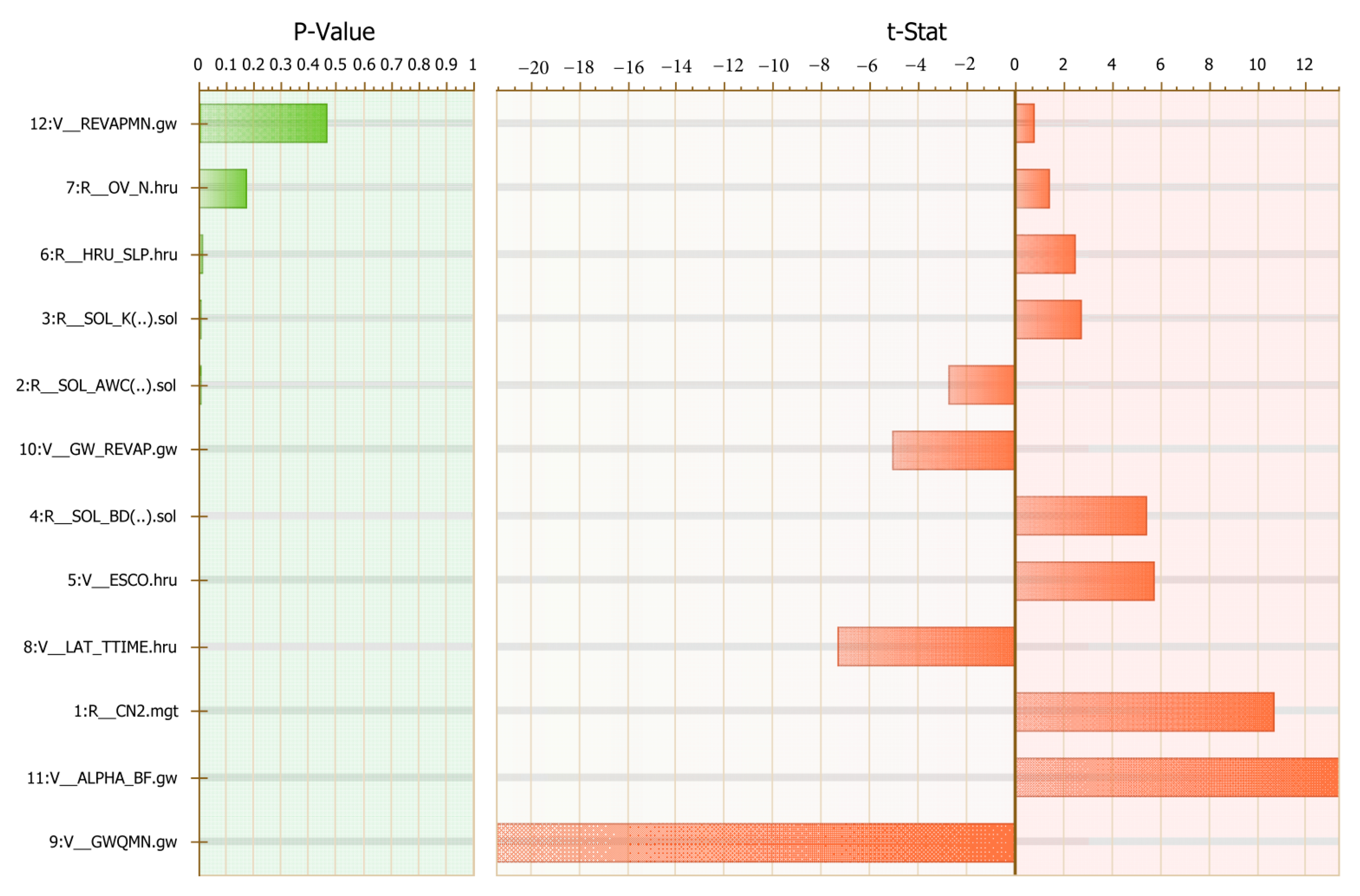
The SWAT performance was carried out using the SWAT-CUP program under the SUFI-2 (Sequential Uncertainty Fitting version 2) procedure and NSE (Nash Sutcliffe Efficiency) function [59] on a monthly basis. First of all, we performed a sensitivity analysis to spot those parameters that exert the most influence on hydrological processes [60]. This stage is important for reducing the uncertainty of model results and accurately executing the calibration and validation procedures [60]. Hence, the global sensitivity analysis included 12 parameters for which two variation methods were chosen, namely ‘v’—which implies the replacement by a given value of the initial value of the existing parameter, and ‘r’—which implies the multiplication by (1+ a given value) of the initial value of the existing parameter [61]. The parameters considered for sensitivity analysis are given in Figure 5.
After performing the sensitivity analysis, we carried out the calibration and validation procedures. The best parameter values as well as their variation interval are given in Table 2. These parameters provide the best values of the objective function.
Overall, we obtained a good SWAT performance after calibration and validation stages, which can be summarized as follows (see [49]: (i) NSE = 0.67, R2 = 0.79, RSR = 0.57, PBIAS = 26.4, p-factor = 0.72, and r-factor = 0.91 for the calibration stage (performed for the 1979–1988 period); and (ii) NSE = 0.65, R2 = 0.66, RSR = 0.59, PBIAS = 2.1, p-factor = 0.75, and r-factor = 1.46 for the validation stage (performed for the 2009–2012 period). A detailed presentation of the SWAT database customization, model setup, calibration, and validation are given in previous work [49].

3.2. Temperature and Precipitation

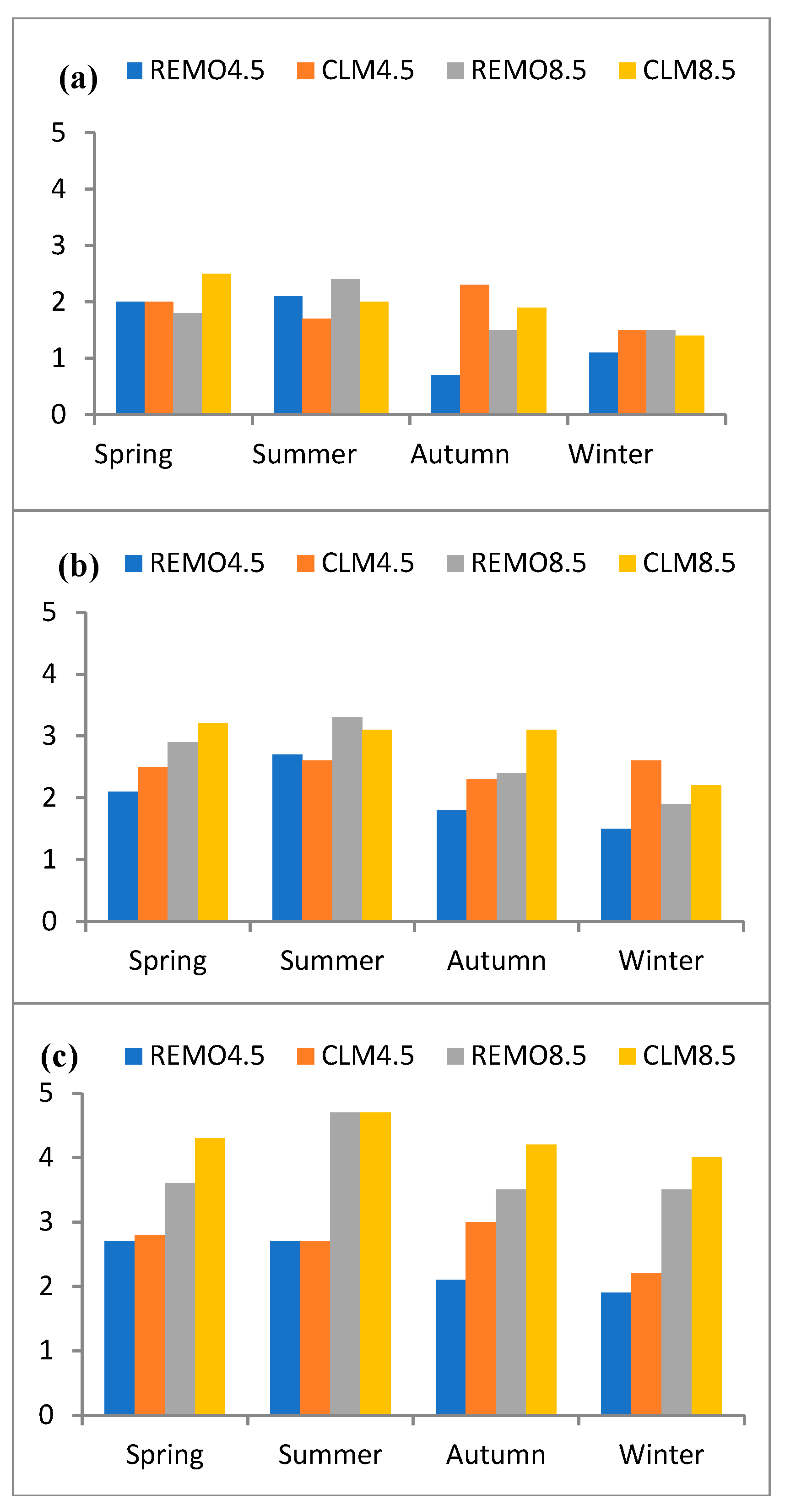
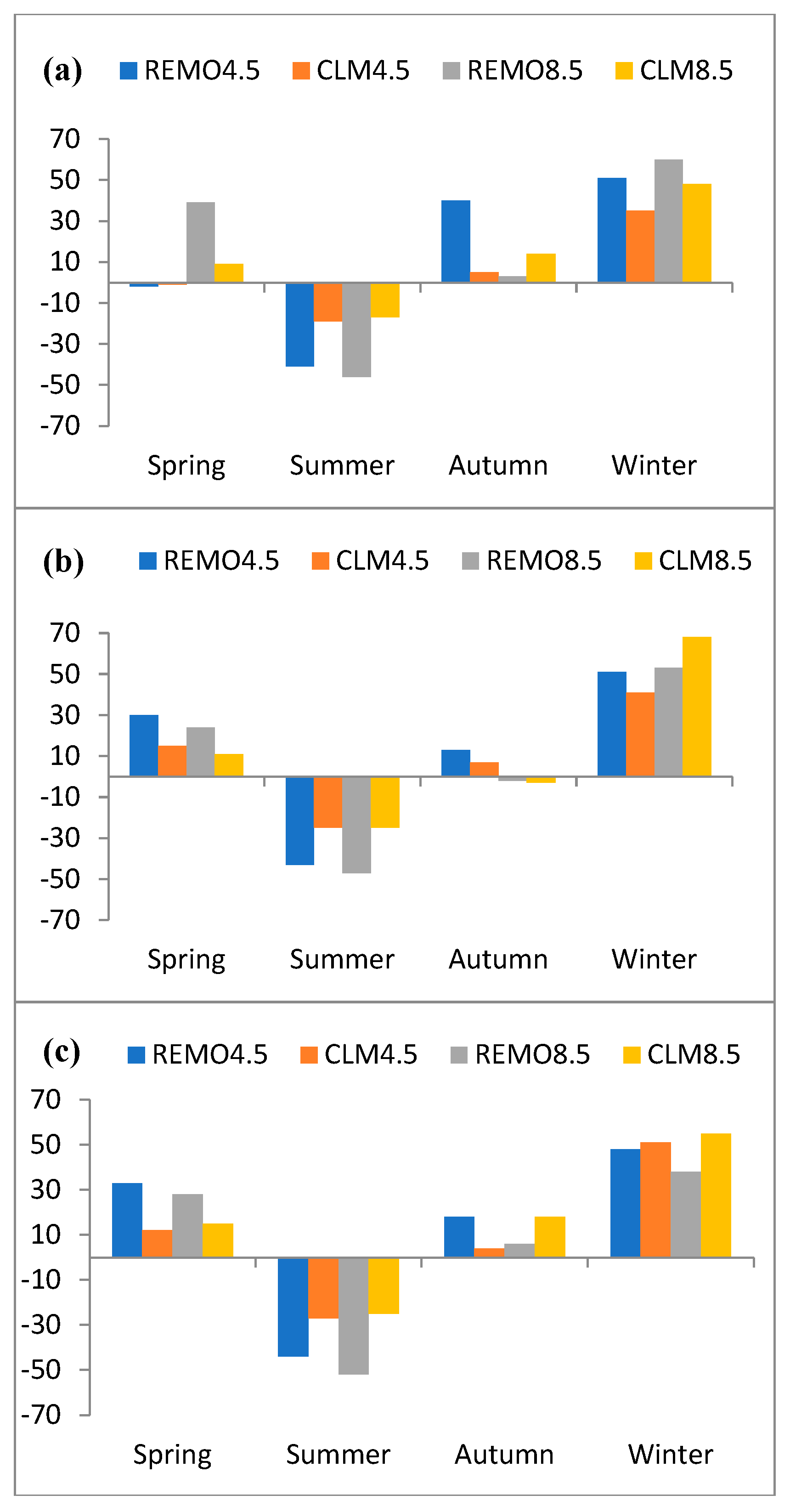
The temperature and precipitation projected for short (2020–2039), mid (2040–2069), and long term (2070–2100) under the GCM–RCM combination models forced by RCP4.5 and RCP8.5 representative concentration pathways are given in Figure 6 and Figure 7 as percentual differences with the baseline period 1979–1988. Figure 6 shows an overall increasing temperature trend projected until 2100. In the short term (Figure 6a), are projected increases in temperature of 0.7 °C (in REMO4.5/autumn) and 2.5 °C (in CLM8.5/spring), the highest values being estimated for spring and summer in REMO and CLM scenarios developed by RCP8.5. Over the mid term (Figure 6b), the temperature is projected to increase by up to 2.7 °C under REMO4.5/summer and up to 3.3 °C under REMO8.5/summer compared with the baseline. In addition, substantial temperature increases are projected over the long term (Figure 6c) when values of 1.9 °C (in REMO4.5/winter) and 4.7 °C (in CLM4.5 and 8.5/summer) higher than baseline are expected. Overall, by the end of the 21st century, the temperature is projected to increase by 1.8–4.3 °C during spring, 1.7–4.7 °C in summer, 0.7–4.2 °C during autumn, and 1.1–4.0 °C in winter.
Instead, for the precipitation (Figure 7), the projections reveal an opposite trend compared with the baseline, with increases by up to 68%, particularly during winter, and decreases by up to 52%, especially in the summer. Over the short term (Figure 7a), compared with the baseline, precipitation is projected either to decrease by 1% (in CLM4.5/spring) and 46% (in REMO8.5/summer) either to increase by 3% (in REMO8.5/autumn) and (in REMO8.5/winter). The mid term (Figure 7b) shows decreases by up to 47% and increases by up to 68%, both projected values in REMO and CLM scenarios developed from RCP8.5 for summer and winter, respectively. A slight 2% and 3% decrease is projected for the autumn precipitation under the REMO8.5 and CLM8.5 scenarios. Over the long term (Figure 7c), the precipitation is projected to increase between 4% (in CLM4.5/autumn) and 55% (in CLM8.5/winter) or to decrease by up to 52% under the REMO8.5 in the summer.

3.3. Seasonal Surface Runoff in the Short Term (2020–2039)

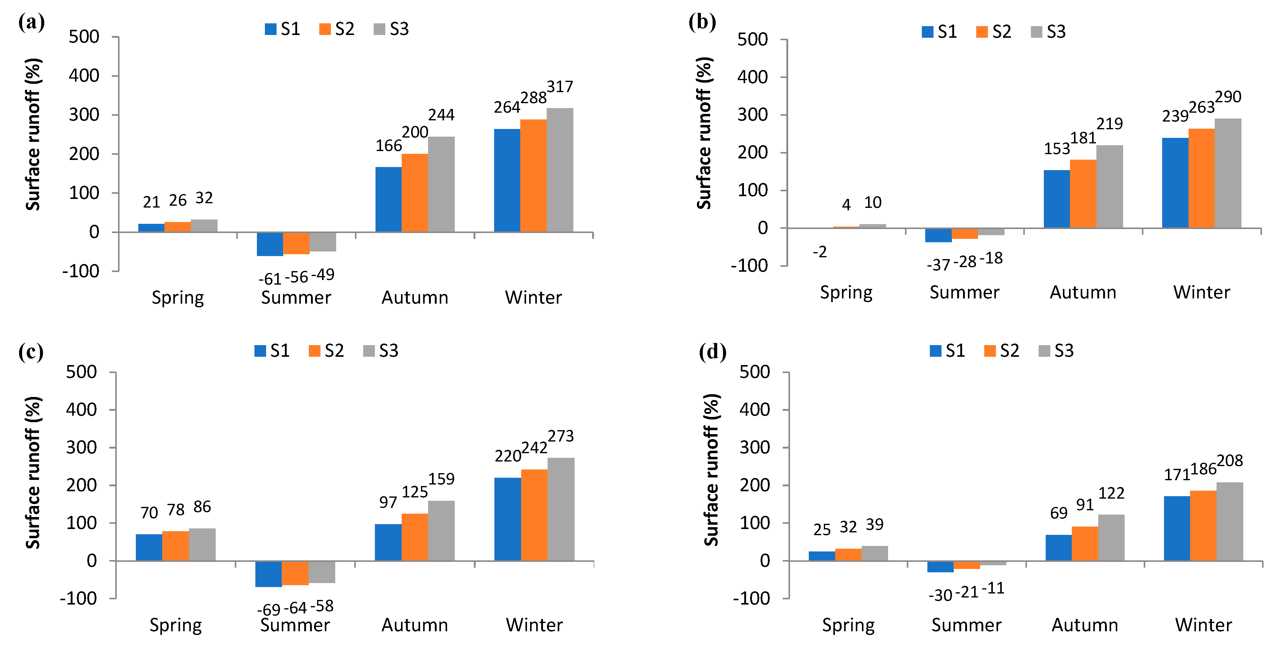
The seasonal surface runoffs projected in the considered scenarios are given in Figure 8a–d as a percentage change compared to the baseline. The results show that, in spring, surface runoff relative changes range from −2% (S1) to 86% (S3) (Figure 8b,c). In summer, the surface runoff decreases, particularly in REMO8.5/S1, when values lower by 69% are projected (Figure 8c). During autumn, increases between 69% (in CLM8.5/S1) and 244% (in REMO4.5/S3) are estimated (Figure 8a,d). A similar trend is also observed for the winter season, where increases of almost 3.2 times compared to the baseline are projected, especially in scenario S3 (Figure 8b).

3.4. Seasonal Surface Runoff in the Mid Term (2040–2069)

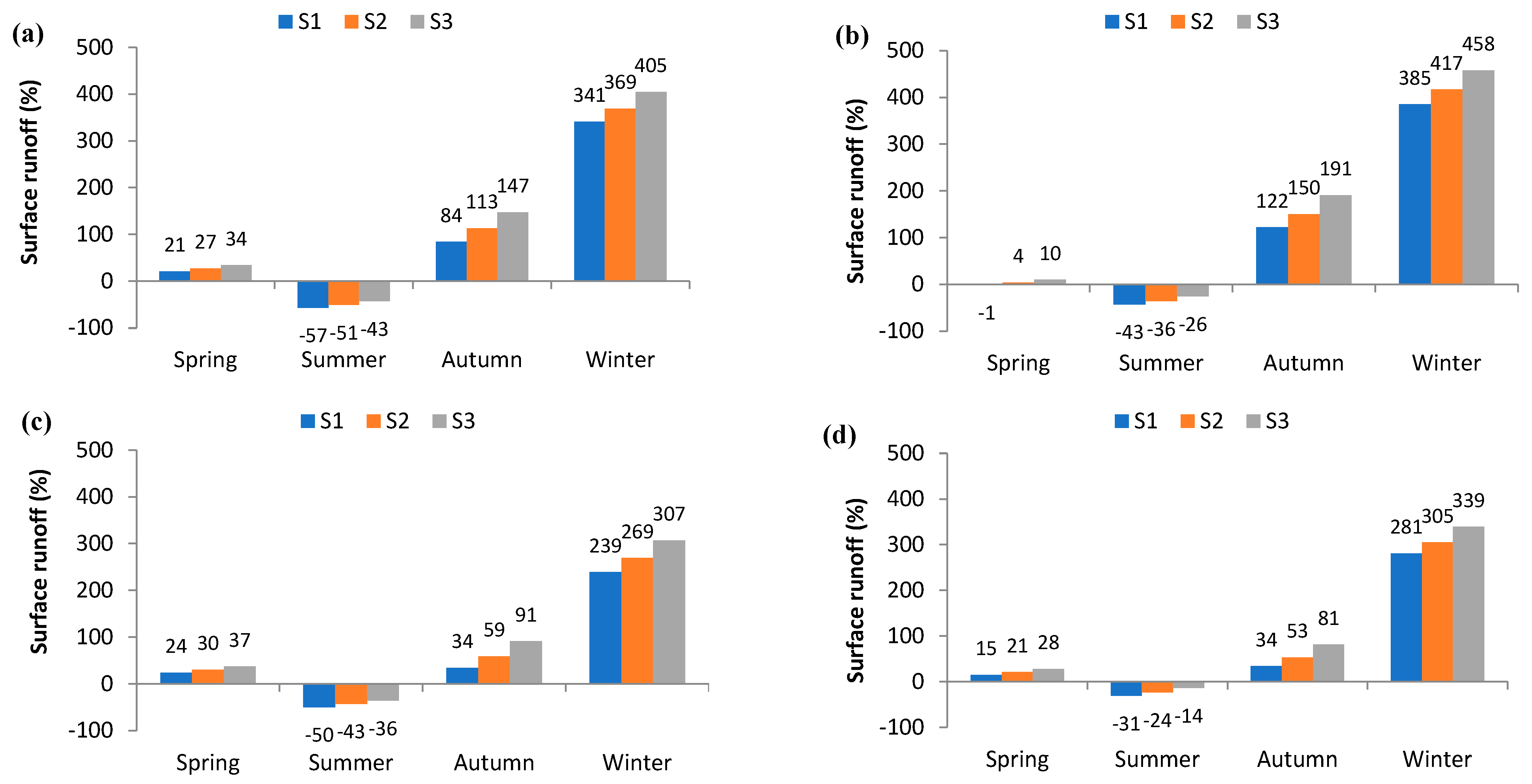
The mid-term simulation of seasonal surface runoff is given in Figure 9a–d. We can observe that, for the spring, either a slight decrease of 1% in CLM4.5/S1 (Figure 9b) or an increase by up to 37% is projected in REMO8.5/S3 (Figure 9c). During the summer months, the surface runoff is expected to decrease between 14–57%, particularly in REMO scenarios coupled with scenario S1. However, in autumn, the surface runoff increases, especially in scenario S3 under REMO4.5 and CLM4.5, a situation that can also be noticed in the winter.

3.5. Seasonal Surface Runoff in the Long Term (2070–2100)

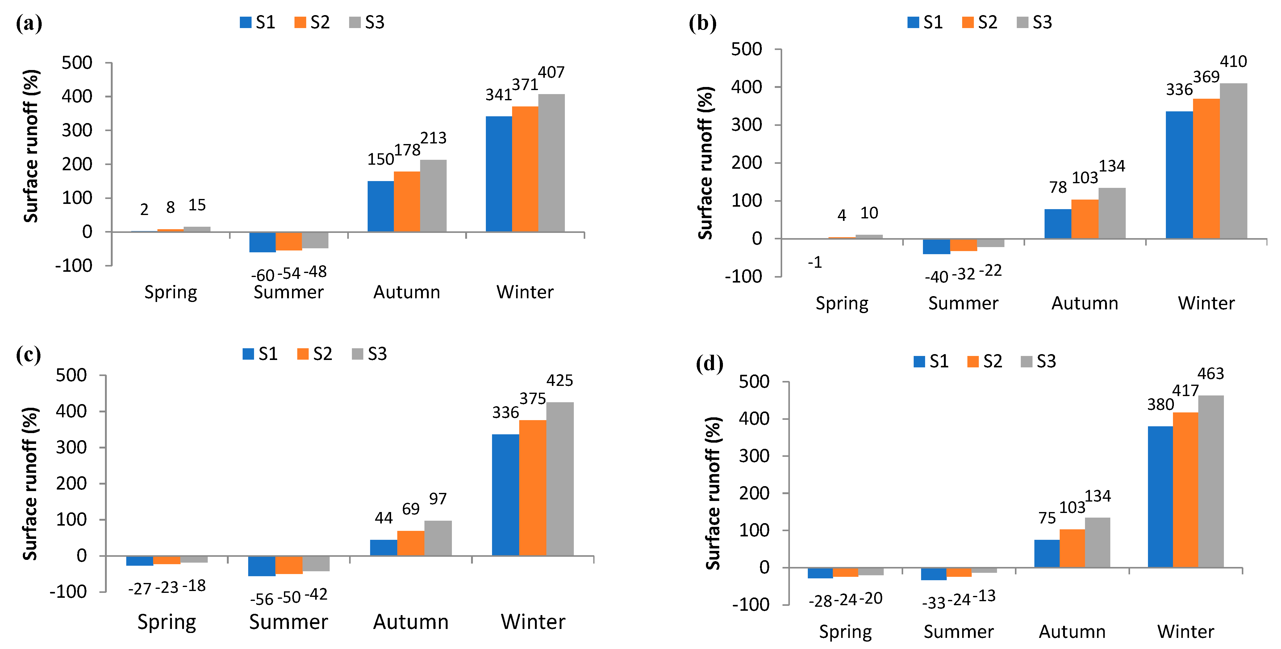
Figure 10a–d illustrates the seasonal surface runoff projected for the long term and shows that the decreasing trend of seasonal surface runoff is mainly projected in scenario S1, while the increments arise particularly in scenarios S2 and S3. For spring, two trends can be observed: increases by up to 15% in REMO4.5 and CLM4.5 (Figure 10a,b) and decreases by up to 18–28% in REMO8.5 and CLM8.5 coupled with scenario S1 (Figure 10b,c). For summer, the surface runoff is projected to decrease between 13–60%, while in autumn, this parameter increases, particularly in REMO4.5 and CLM4.5 (Figure 10a,b). During the winter, the most pronounced increases in surface runoff are projected, with values four times higher than the estimated baseline (Figure 10d).

3.6. Surface Runoff Data Analysis

In order to assess the trends regarding surface runoff under climate and land use scenarios, we use statistical analysis (based on STATISTICA 13.5.0.17) to capture the evolution trend. We used One-Way ANOVA to test the influences. If the precondition of the parametric test was not met, we applied the Kruskal–Wallis non-parametric test. Among climate change scenarios, significant differences in surface runoff appear only in REMO8.5 (Table 3). The differences in the surface runoff between the other climate change scenarios applied are insignificant.
Assessing the influence of land use scenarios (S1–S3), we noticed that, for the 2020–2100 period, significant differences in the surface runoff appeared only in the S1 scenario (Table 4).
At the seasonal level, we noticed that significant differences in surface runoff appear only during spring and winter (Table 5).

4. Discussion and Conclusions

Worldwide, climate change triggers important modification that impacts water resources. The projected increases in air temperature, the varied precipitation across regions, and more frequent and intense extreme events will modify the water cycle and reduce water availability in the future [29,62]. Furthermore, exacerbated by the changes in land use, hydrological processes will be negatively affected both in the short, mid, and long term [5]. Thus, it is imperative to understand the watershed response to climate and land use change and to establish adaptive measures for sustainable management. Nonetheless, for reliable projections, it is essential to use high-resolution models and methods that accurately capture the local and regional conditions [63,64]. Considering the higher vulnerability of small forested watersheds located in a mountainous area to climate change and land use change [57,65,66,67], future assessments of those impacts on watershed hydrological balances are imperative for sustainable management mainly due to the limited studies that address seasonal dynamics of the hydrological process [20].
Therefore, in this study, we used the SWAT model to investigate the changes in the seasonal surface runoff for a small forested watershed in a mountainous area in central Romania which represents the main water source for approximately 473,000 inhabitants. After obtaining a good model performance to simulate hydrological processes within the Upper Tarlung watershed [49], we developed future climate and land use change scenarios [51,53]. Finally, these scenarios were embedded into the calibrated and validated SWAT model for projecting seasonal surface runoff from 2020–2100 was divided into short (2020–2039), mid (2040–2069), and long-term (2070–2100) periods.

4.1. Changes in Temperature and Precipitation

The future climate derived from GCM–RCM combination models for RCP4.5 and RCP8.5 representative concentration pathways foresee increases in temperature by up to 2.5 °C in the short term, up to 3.3 °C in the midterm, and by up to 4.7 °C in the long term which corresponds to global climate projections. This corroborates the findings of Sfîcă et al. [68] who reported increases in air temperatures over 4 °C by the end of the century within Romania. The highest increases are estimated under scenarios developed from RCP8.5 and for the summer season. Those findings correspond with the results of other studies carried out for our country, which emphasized that, in the future, the climate will be warmer and heatwave frequency and intensity will increase [3,40,57,69], with more pronounced tendencies towards the end of the century [57,70].
Unlike for temperature, the projected precipitation showed opposite trends, which are similar to the findings of other studies [3,57,71]. However, those projections differ in relation to the climate scenarios and the period of time or considered season. The highest increases are expected during the winter, while the sharpest decreases are estimated for summer, both tendencies being more pronounced in scenarios developed from RCP8.5. Those findings contrast the results of other studies [62,72], which reported that precipitation would increase during summer and decrease in winter. Decreases in summer precipitation disagree with the results of other studies [46,62] that reported increases in summer amounts but corresponded with the findings of [69] that obtained the sharpest decreases in the RCP8.5 scenario by the end of the century. Instead, the projected changes show both increases and decreases for spring and autumn, which can be noticed only in the short and midterm. Those findings are consistent with the results of [70] that obtained a similar seasonal variation of the precipitation projected until 2100.

4.2. Changes in Seasonal Surface Runoff

The model outputs show that seasonal surface runoff predicted in the short term (Figure 8) is projected to decrease by up to 69% or an increase up to threefold compared with the baseline value. In spring, the surface runoff may slightly decrease by 2% or increase by up to 86%, which could be justified by the snowmelt process as stated in previous studies [62,73]. The summer surface runoff decreases by up to 69%, the largest decrease over the entire analyzed period (until 2100). This result disagrees with the projections of [73], who estimated the sharpest decreases in summer runoff towards the end of the century, probably caused by precipitation amounts in that period and lower groundwater recharge during winter due to reduced snowpack. For autumn, we obtained increases of surface runoff around twice at large compared to baseline, while during winter the surface runoff can increase around threefold compared to the baseline, the highest increases being obtained under the moderate RCP4.5 scenarios. We believe that winter runoff increases are mainly due to the predicted changes in temperature and precipitation, which favors the occurrence of more liquid and not solid rain and faster snowmelt that trigger a more consistent surface runoff. This aspect was also mentioned in other studies [62,70,73,74]. Those increases can also be attributed to the land use change as it is well known that the reduction of forested areas has a great potential to generate more intense surface runoff [19,75,76]. For the entire considered period, it can be observed that the overall decreasing trend is more accentuated in scenario S1, while scenario S3 can lead to the most accentuated increases in surface runoff. Thus, we can state that land use change has a much greater influence on surface runoff compared to changes in climate conditions, which confirms the findings of [47].
Regarding seasonal surface runoff projected for the mid term (Figure 9), we observe that surface runoff during the spring shows a similar pattern as the previous period, except for a lower increase (up to 37%). Opposing tendencies in spring runoff and the lowest increases of surface runoff in spring from all seasons were also reported by [77]. In summer, the surface runoff can decrease by up to 57%, which can be attributed to the increased temperature that intensifies the evapotranspiration rate and the decreased precipitation estimated for this period [3,62]. For autumn, increases in surface runoff twice as large as the baseline are estimated—particularly in scenarios from RCP4.5. We noticed that the most consistent increases are projected for the winter months, similar findings being also reported by [77]. This situation could be related to the projected increases in temperature (up to 2.6 °C) and precipitation (up to 70%) that generated a greater volume of liquid precipitation and faster snowmelt, as suggested by other studies [62,74]. For the entire period, we noticed that scenarios developed from RCP4.5 generated the most pronounced surface runoff increases and decreases. Regarding the land use change, we observed that scenario S1 generates the most significant decreases, while the increases are more pronounced in scenario S3.
The modeled seasonal surface runoff over the long term (Figure 10) revealed that for spring, there were projected increases by up to 15% or decreases by up to 28%. The decreased tendency in spring runoff was also reported by [77] which estimated decreases by up to 26%, while our projections show a reduction by up to 28%. Our findings correspond with the results of [71] that reported for the 2071–2100 period a different behavior of surface runoff for spring. Unlike their results, we obtained the increased trend of spring runoff only in the scenarios developed from RCP4.5 [71], probably due to different watershed characteristics and runoff regime. We found that the most significant decreases in spring runoff were estimated in scenarios developed from RCP8.5. Similar findings were reported in [73]. The decreased tendency of spring runoff can be attributed to reduced snowfall, as suggested by [78]. In summer, the surface runoff can decrease by up to 60%, with a similar result reported in other studies [73,77]. In autumn, surface runoff can increase by twice as much as the baseline value, especially in scenarios developed from RCP4.5. In winter, the increases of this parameter by 3.4–4.7 times compared to the baseline are projected, a result that is in line with the findings of [73] but in disagreement with the results of [78] that estimate the largest runoff increases for the spring season, justified by the authors as a consequence of increased precipitation and snowmelt. However, increases in surface runoff during autumn and winter and considerable decreases in the summer season were also reported by [71]. The consistent increases during wintertime could be related to the temperature and precipitation increases, as highlighted in previous studies [62,74,78].
Simulations performed for three future periods (2020–2039, 2040–2069, 2070–2100) were analyzed compared to the reference period (1979–1988). The records of flow measurement were available for the 1974–2014 period but in an incomplete format. For this interval, we had continuous flow measurements and identified periods with dry, average, and rainy years as is recommended in the literature [58]. Overall, climate and land use changes modify seasonal surface runoff regardless of the time period considered, and it can be seen that the decreasing trend is more accentuated in scenario S1, which shows decreases of up to 69% of the surface runoff, while the increases are more pronounced, particularly in scenario S3, when values up to five times fold are expected, especially during winter. Furthermore, the modeling activities pointed out opposite tendencies for spring runoff, considerable decreases during summer, and an increasing trend for autumn which will peak during winter. The reduced values in surface runoff during the summer, up to approximately 70% lower than the reference values, suggest the possibility of droughts in the 2020–2100 period. Contrastingly, during autumn and winter especially, important increases in surface runoff, when values five times fold approximately compared to baseline are projected, can lead to flood occurrence of floods in those periods. Benefiting from these projections, decision-makers can adopt certain measures to reduce or mitigate the occurrence of these extreme events. Those findings contribute to an increased understanding of climate and land use change impact on surface runoff on a seasonal level in small forested watersheds, which are important for local water managers that can anticipate and reduce the adverse effects, such as floods or droughts. The results can be used as a basis to design adaptation strategies related to climate and land use change impacts in a mountainous watershed and are also important for forest managers in optimizing land use categories so that water resources can be secured in the following years.
Although the SWAT model was initially developed for large river basins (>10,000 km2), it was successfully applied in the studied watershed with an area of up to 100 km2. Moreover, we obtained a good model performance in simulating hydrological processes. Additionally, the studied watershed is located in a mountainous area and is not equipped with conventional gauges for continuous measurements of flows. In this context, the SWAT model has the advantage of requesting few input data that are easily accessible and provides easy access to information on hydrological parameters. Therefore, this study delivers valuable insights for local decision-makers that are sustained to adopt coherent strategies considering long-term climate informed decisions. Besides, to the best of our knowledge, our study is so far the first one performed at a national level that customizes soil and land use databases at the compartment level unit and applies SWAT in a watershed with an area of up to 100 km2. In addition, this study tries to fill the gap in relation to the limited number of studies that address seasonal surface runoff, the majority of them being focused on annual evaluations. Therefore, our findings are useful and can support local decision-makers responsible for watershed management in conceiving sound strategies to avoid unwanted consequences brought about by changes in climate or land use. Even if the reduction of the forest area is possible but improbable over the next eight decades, this study highlights the importance of forests in mitigating the harmful effects of climate change. Therefore, all institutions responsible for managing the land use within the studied watershed should consider preserving the current land use categories as much as possible and promote optimal management from the hydrological point of view. Moreover, in the climate change context, decision-makers should advocate for increasing the forested areas within the studied watershed, considering the fundamental role of forests in alleviating the impact of climate change. The research outputs offer decision-makers the possibility to spatially (at subwatershed level) and temporally (depending on decades with hydrological risk) stagger the intervention with torrent control structures of the torrential hydrographic network. At the same time, the modeling activities allow establishing the limits of land exploitation considering the land use categories (animal husbandry, forest production, clean water production, and biodiversity) to be established.

Author Contributions

Conceptualization, M.M. and I.C.; methodology, M.M., N.C.T. and C.U.; software, M.M. and N.C.T.; validation, M.M. and I.C.; formal analysis, M.M., N.C.T. and C.U.; investigation, M.M.; resources, M.M. and N.C.T.; data curation, M.M., N.C.T. and C.U.; writing—original draft preparation, M.M.; writing—review and editing, M.M.; visualization, N.C.T., A.L.M., N.E.M. and O.N.T.; supervision, N.C.T. and I.C.; project administration, N.C.T. and I.C.; funding acquisition, N.C.T. All authors have read and agreed to the published version of the manuscript.

Funding

The present research benefits from funding from the project Climate Services for Water-Energy-Land-Food Nexus (CLISWELN) funded by ERA4CS. ERA4CS is an ERA-NET initiated by JPI Climate, and CLISWELN is funded by Bundesministerium für Bildung und Forschung (BMBF-Germany), Executive Agency for Higher Education, Research, Development, and Innovation Funding (UEFISCDI -Romania), Bundesministerium für Bildung, Wissenschaft und Forschung and ¨Osterreichische Forschungsf¨orderungsgesellschaft (BMBWF and FFG Austria), and Ministerio de Economía y Competitividad (MINECO Spain), with co-funding from the European Union’s Horizon 2020 under Grant Agreement No 690462. This work was also supported by “CresPerfInst” (Contract no. 34PFE./30.12.2021—Increasing the institutional capacity and performance of INCDS “Marin Drăcea” in the activity of RDI) and Grant Agreement No-PN19070404 ’Gestionarea integrată a terenurilor forestiere și albiilor în vederea reducerii riscurilor induse de excedentul de apă’ funded from the Ministry of Research and Innovation.

Institutional Review Board Statement

Not applicable.

Informed Consent Statement

Not applicable.

Data Availability Statement

Not applicable.

Conflicts of Interest

The authors declare no conflict of interest.

References

  1. Arias, P.A.; Bellouin, N.; Coppola, E.; Jones, R.G.; Krinner, G.; Marotzke, J.; Naik, V.; Palmer, M.D.; Plattner, G.-K.; Rogelj, J.; et al. Technical Sumary. In Climate Change 2021: The Physical Science Basis; Contribution of Working Group I to the Sixth Assessment Report of the Intergovernmental Panel on Climate Change; Cambridge University Press: Cambridge, UK; New York, NY, USA, 2021; pp. 33–144. [Google Scholar] [CrossRef]
  2. IPCC Summary for Policymakers. In Climate Change 2021: The Physical Science Basis; Contribution of Working Group I to the Sixth Assessment Report of the Intergovernmental Panel on Climate Change; Cambridge University Press: Cambridge, UK; New York, NY, USA, 2021; pp. 3–32. [CrossRef]
  3. Cheval, S.; Dumitrescu, A.; Bîrsan, M.V. Variability of the aridity in the South-Eastern Europe over 1961–2050. Catena 2017, 151, 74–86. [Google Scholar] [CrossRef]
  4. Sfîcă, L.; Croitoru, A.E.; Iordache, I.; Ciupertea, A.F. Synoptic conditions generating heatwaves and warm spells in Romania. Atmosphere 2017, 8, 50. [Google Scholar] [CrossRef]
  5. Marin, M.; Clinciu, I.; Tudose, N.; Ungurean, C.; Adorjani, A.; Mihalache, A.; Davidescu, A.; Davidescu, Ș.O.; Dinca, L.; Cacovean, H. Assessing the vulnerability of water resources in the context of climate changes in a small forested watershed using SWAT: A review. Environ. Res. 2020, 184, 109330. [Google Scholar] [CrossRef]
  6. Yao, J.; Chen, Y.; Guan, X.; Zhao, Y.; Chen, J.; Mao, W. Recent climate and hydrological changes in a mountain–basin system in Xinjiang, China. Earth-Sci. Rev. 2022, 226, 103957. [Google Scholar] [CrossRef]
  7. Ducci, F.; De Rogatis, A.; Proietti, R.; Curtu, A.L.; Marchi, M.; Belletti, P. Establishing a baseline to monitor future climate-change-effects on peripheral populations of Abies alba in central Apennines. Ann. For. Res. 2021, 64, 33–66. [Google Scholar] [CrossRef]
  8. Kutnar, L.; Kermavnar, J.; Pintar, A.M. Climate change and disturbances will shape future temperate forests in the transition zone between Central and SE Europe. Ann. For. Res. 2021, 64, 67–86. [Google Scholar] [CrossRef]
  9. Kwarteng, E.A.; Gyamfi, C.; Anyemedu, F.O.K.; Adjei, K.A.; Anornu, G.K. Coupling SWAT and bathymetric data in modelling reservoir catchment hydrology. Spat. Inf. Res. 2021, 29, 55–69. [Google Scholar] [CrossRef]
  10. Tian, J.; Guo, S.; Deng, L.; Yin, J.; Pan, Z.; He, S.; Li, Q. Adaptive optimal allocation of water resources response to future water availability and water demand in the Han River basin, China. Sci. Rep. 2021, 11, 7879. [Google Scholar] [CrossRef]
  11. Liu, J.; Xue, B.; Yan, Y. The assessment of climate change and land-use influences on the runoff of a typical coastal basin in Northern China. Sustainability 2020, 12, 10050. [Google Scholar] [CrossRef]
  12. UNDP. Sustainable Development Goals; UNDP: New York, NY, USA, 2015. [Google Scholar]
  13. United Nations. Progress towards the Sustainable Development Goals Report of the Secretary-General; United Nations: New York, NY, USA, 2022. [Google Scholar]
  14. Dong, Z.; Zhang, J.; Zhang, K.; Wang, X.; Chen, T. Multi-objective optimal water resources allocation in the middle and upper reaches of the Huaihe River Basin (China) based on equilibrium theory. Sci. Rep. 2022, 12, 6606. [Google Scholar] [CrossRef]
  15. Munoth, P.; Goyal, R. Impacts of land use land cover change on runoff and sediment yield of Upper Tapi River Sub-Basin, India. Int. J. River Basin Manag. 2020, 18, 177–189. [Google Scholar] [CrossRef]
  16. Sidău, M.R.; Horváth, C.; Cheveresan, M.; Șandric, I.; Stoica, F. Assessing hydrological impact of forested area change: A remote sensing case study. Atmosphere 2021, 12, 817. [Google Scholar] [CrossRef]
  17. Tan, X.; Liu, S.; Tian, Y.; Zhou, Z.; Wang, Y.; Jiang, J.; Shi, H. Impacts of Climate Change and Land Use/Cover Change on Regional Hydrological Processes: Case of the Guangdong-Hong Kong-Macao Greater Bay Area. Front. Environ. Sci. 2022, 9, 2411–2502. [Google Scholar] [CrossRef]
  18. Bian, G.; Wang, G.; Chen, J.; Zhang, J.; Song, M. Spatial and seasonal variations of hydrological responses to climate and land-use changes in a highly urbanized basin of Southeastern China. Hydrol. Res. 2021, 52, 506–522. [Google Scholar] [CrossRef]
  19. Guzha, A.C.; Rufino, M.C.; Okoth, S.; Jacobs, S.; Nóbrega, R.L.B. Impacts of land use and land cover change on surface runoff, discharge and low flows: Evidence from East Africa. J. Hydrol. Reg. Stud. 2018, 15, 49–67. [Google Scholar] [CrossRef]
  20. Ouyang, L.; Liu, S.; Ye, J.; Liu, Z.; Sheng, F.; Wang, R.; Lu, Z. Quantitative assessment of surface runoff and base flow response to multiple factors in Pengchongjian Small watershed. Forests 2018, 9, 553. [Google Scholar] [CrossRef]
  21. Aghapour Sabbaghi, M.; Nazari, M.; Araghinejad, S.; Soufizadeh, S. Economic impacts of climate change on water resources and agriculture in Zayandehroud river basin in Iran. Agric. Water Manag. 2020, 241, 106323. [Google Scholar] [CrossRef]
  22. Nielsen-Gammon, J.W.; Banner, J.L.; Cook, B.I.; Tremaine, D.M.; Wong, C.I.; Mace, R.E.; Gao, H.; Yang, Z.L.; Gonzalez, M.F.; Hoffpauir, R.; et al. Unprecedented Drought Challenges for Texas Water Resources in a Changing Climate: What Do Researchers and Stakeholders Need to Know? Earth’s Futur. 2020, 8, 8. [Google Scholar] [CrossRef]
  23. Gemechu, T.M.; Zhao, H.; Bao, S.; Yangzong, C.; Liu, Y.; Li, F.; Li, H. Estimation of hydrological components under current and future climate scenarios in guder catchment, upper Abbay Basin, Ethiopia, using the swat. Sustainability 2021, 13, 9689. [Google Scholar] [CrossRef]
  24. Wu, J.; Miao, C.; Zhang, X.; Yang, T.; Duan, Q. Detecting the quantitative hydrological response to changes in climate and human activities. Sci. Total Environ. 2017, 586, 328–337. [Google Scholar] [CrossRef]
  25. Wang, Q.; Xu, Y.; Xu, Y.; Wu, L.; Wang, Y.; Han, L. Spatial hydrological responses to land use and land cover changes in a typical catchment of the Yangtze River Delta region. CATENA 2018, 170, 305–315. [Google Scholar] [CrossRef]
  26. Chilagane, N.; Kashaigili, J.; Mutayoba, E.; Lyimo, P.; Munishi, P.; Tam, C.; Burgess, N. Impact of Land Use and Land Cover Changes on Surface Runoff and Sediment Yield in the Little Ruaha River Catchment. Open J. Mod. Hydrol. 2021, 11, 54–74. [Google Scholar] [CrossRef]
  27. Phung, Q.A.; Thompson, A.L.; Baffaut, C.; Costello, C.; Sadler, E.J.; Svoma, B.M.; Lupo, A.; Gautam, S. Climate and Land Use Effects on Hydrologic Processes in a Primarily Rain—Fed, Agricultural Watershed. JAWRA J. Am. Water Resour. Assoc. 2019, 55, 1196–1215. [Google Scholar] [CrossRef]
  28. OECD. Water Resources Allocation: Sharing Risks and Opportunities; OECD: Paris, France, 2015; Volume 14. [Google Scholar]
  29. Jeyrani, F.; Morid, S.; Srinivasan, R. Assessing basin blue–green available water components under different management and climate scenarios using SWAT. Agric. Water Manag. 2021, 256, 107074. [Google Scholar] [CrossRef]
  30. Abbaspour, K.C.; Rouholahnejad, E.; Vaghefi, S.; Srinivasan, R.; Yang, H.; Kløve, B. A continental-scale hydrology and water quality model for Europe: Calibration and uncertainty of a high-resolution large-scale SWAT model. J. Hydrol. 2015, 524, 733–752. [Google Scholar] [CrossRef]
  31. Fu, B.; Merritt, W.S.; Croke, B.F.W.; Weber, T.R.; Jakeman, A.J. A review of catchment-scale water quality and erosion models and a synthesis of future prospects. Environ. Model. Softw. 2019, 114, 75–97. [Google Scholar] [CrossRef]
  32. Cakir, R.; Raimonet, M.; Sauvage, S.; Paredes-Arquiola, J.; Grusson, Y.; Roset, L.; Meaurio, M.; Navarro, E.; Sevilla-Callejo, M.; Lechuga-Crespo, J.L.; et al. Hydrological alteration index as an indicator of the calibration complexity ofwater quantity and quality modeling in the context of global change. Water 2020, 12, 115. [Google Scholar] [CrossRef]
  33. Gassman, P.W.; Sadeghi, A.M.; Srinivasan, R. Applications of the SWAT Model Special Section: Overview and Insights. J. Environ. Qual. 2014, 43, 1–8. [Google Scholar] [CrossRef]
  34. Arnold, J.G.; Srinivasan, R.; Muttiah, R.S.; Williams, J.R. Large area hydrologic modelind and assesssment. Part I: Model Development. J. Am. Water Resour. Assoc. 1998, 34, 73–89. [Google Scholar] [CrossRef]
  35. Gassman, P.W.; Reyes, M.R.; Green, C.H.; Arnold, J.G.; Gassman, P.W. The soil and water assessment tool: HISTORICAL development, applications, and future research directions invited review series. Trans. ASABE 2007, 50, 1211–1250. [Google Scholar] [CrossRef]
  36. Arnold, J.G.; Moriasi, D.N.; Gassman, P.W.; Abbaspour, K.C.; White, M.J.; Srinivasan, R.; Santhi, C.; Harmel, R.D.; Van Griensven, A.; Van Liew, M.W.; et al. SWAT: Model use, calibration, and validation. Trans. ASABE 2012, 55, 1491–1508. [Google Scholar] [CrossRef]
  37. Arnold, J.G.; Kiniry, J.R.; Srinivasan, R.; Williams, J.R.; Haney, E.B.; Neitsch, S.L. Soil & Water Assessment Tool. In Input/Output Documentation; Springer: Berlin/Heidelberg, Germany, 2012. [Google Scholar]
  38. Narula, K.K.; Nischal, S. Hydrological Modelling of Small Gauged and Ungauged Mountainous Watersheds Using SWAT—A Case of Western Ghats in India. J. Water Resour. Prot. 2021, 13, 455–477. [Google Scholar] [CrossRef]
  39. Micu, D.M.; Amihaesei, V.A.; Milian, N.; Cheval, S. Recent changes in temperature and precipitation indices in the Southern Carpathians, Romania (1961–2018). Theor. Appl. Climatol. 2021, 144, 691–710. [Google Scholar] [CrossRef]
  40. Nagavciuc, V.; Scholz, P.; Ionita, M. Hotspots for warm and dry summers in Romania. Nat. Hazards Earth Syst. Sci. 2021, 22, 1347–1369. [Google Scholar] [CrossRef]
  41. Duvillard, P.A.; Ravanel, L.; Marcer, M.; Schoeneich, P. Recent evolution of damage to infrastructure on permafrost in the French Alps. Reg. Environ. Chang. 2019, 19, 1281–1293. [Google Scholar] [CrossRef]
  42. Bîrsan, M.-V.; Dumitrescu, A. Snow variability in Romania in connection to large—scale atmospheric circulation. Int. J. Climatol. 2014, 34, 134–144. [Google Scholar] [CrossRef]
  43. Sajikumar, N.; Remya, R.S. Impact of land cover and land use change on runoff characteristics. J. Environ. Manage 2015, 161, 460–468. [Google Scholar] [CrossRef]
  44. Liu, Y.; Xu, Y.; Zhao, Y.; Long, Y. Using SWAT Model to Assess the Impacts of Land Use and Climate Changes on Flood in the Upper Weihe River, China. Water 2022, 14, 2098. [Google Scholar] [CrossRef]
  45. Wu, Y.; He, G.; Ouyang, W.; Huang, L. Differences in soil water content and movement drivers of runoff under climate variations in a high-altitude catchment. J. Hydrol. 2020, 587, 125024. [Google Scholar] [CrossRef]
  46. Strohmenger, L.; Ackerer, P.; Belfort, B.; Pierret, M.C. Local and seasonal climate change and its influence on the hydrological cycle in a mountainous forested catchment. J. Hydrol. 2022, 610, 127914. [Google Scholar] [CrossRef]
  47. Kiprotich, P.; Wei, X.; Zhang, Z.; Ngigi, T.; Qiu, F.; Wang, L. Assessing the Impact of Land Use and Climate Change on Surface Runoff Response Using Gridded Observations and SWAT+. Hydrology 2021, 8, 48. [Google Scholar] [CrossRef]
  48. Tudose, N.C.; Marin, M.; Cheval, S.; Ungurean, C.; Davidescu, S.O.; Tudose, O.N.; Mihalache, A.L.; Davidescu, A.A. SWAT Model Adaptability to a Small Mountainous Forested Watershed in Central Romania. Forests 2021, 12, 860. [Google Scholar] [CrossRef]
  49. Marin, M.; Clinciu, I.; Tudose, N.C.; Davidescu, S.O.; Constandache, C. Assessing the performance of the Soil and Water Assessment Tool hydrological model for a small mountain forested watershed in the central part of Romania. In Proceedings of the Geolinks Multidisciplinary International Scientific Conference. Conference Proceedings, Novotel, Athens, Greece, 26–29 March 2019; pp. 265–273. [Google Scholar]
  50. Hibbert, A.R. Forest treatment effects on water yield. In Forest Hydrology; Proceedings of A National Science Foundation Advanced Science Seminar; Pergamon Press: Oxford, UK, 1967; pp. 527–543. [Google Scholar]
  51. Marin, M.; Clinciu, I.; Tudose, N.; Cheval, S.; Ungurean, C.; Davidescu, Ș.O.; Adorjani, A.; Mihalache, A.; Davidescu, A.; Tudose, O. Simularea impactului schimbărilor climatice și al modificării folosinței terenului asupra proceselor hidrologice din bazinul hidrografic Tărlungul Superior. Rev. Pădurilor 2020, 135, 1–26. [Google Scholar]
  52. Tudose, N.; Ungurean, C.; Davidescu, Ș.; Cheval, S.; Marin, M. Information Tailored to the Needs of Stakeholders in the Romanian Case Study. Deliverable 4.3. CLISWELN Project. Available online: https://www.hzg.de/ms/clisweln/075105/index.php.en. (accessed on 17 June 2022).
  53. Marin, M.; Clinciu, I.; Tudose, N.C.; Cheval, S.; Ungurean, C.; Davidescu, Ș.O.; Adorjani, A.; Mihalache, A.L.; Davidescu, A.A.; Tudose, O.N. Analiza previziunilor privind regimul termic și pluvial din bazinul hidrografic Tărlungul Superior în contextul schimbărilor climatice. Rev. Silvic. si Cineg. 2019, 45, 15–21. [Google Scholar]
  54. Michelangeli, P.A.; Vrac, M.; Loukos, H. Probabilistic downscaling approaches: Application to wind cumulative distribution functions. Geophys. Res. Lett. 2009, 36, L11708. [Google Scholar] [CrossRef]
  55. Gudmundsson, L.; Bremnes, J.B.; Haugen, J.E.; Engen Skaugen, T. Technical Note: Downscaling RCM precipitation to the station scale using quantile mapping—a comparison of methods. Hydrol. Earth Syst. Sci. Discuss. 2012, 9, 6185–6201. [Google Scholar] [CrossRef]
  56. Luo, M.; Liu, T.; Meng, F.; Duan, Y.; Frankl, A.; Bao, A.; De Maeyer, P. Comparing Bias Correction Methods Used in Downscaling Precipitation and Temperature from Regional Climate Models: A Case Study from the Kaidu River Basin in Western China. Water 2018, 10, 1046. [Google Scholar] [CrossRef]
  57. Tudose, N.C.; Cheval, S.; Ungurean, C.; Broekman, A.; Sanchez-Plaza, A.; Cremades, R.; Mitter, H.; Kropf, B.; Davidescu, S.O.; Dinca, L.; et al. Climate services for sustainable resource management: The water—energy—land nexus in the Tărlung river basin (Romania). Land Use Policy 2022, 119, 106221. [Google Scholar] [CrossRef]
  58. Gan, T.Y.; Dlamini, E.M.; Biftu, G.F. Effects of model complexity and structure, data quality, and objective functions on hydrologic modeling. J. Hydrol. 1997, 192, 81–103. [Google Scholar] [CrossRef]
  59. Abbaspour, K.C.; Vejdani, M.; Haghighat, S. SWAT-CUP Calibration and Uncertainty Programs for SWAT. In Proceedings of the Modsim 2007: International Congress on Modelling and Simulation, Christchurch, New Zealand, 10–13 December 2007; pp. 1603–1609. [Google Scholar]
  60. Gan, Y.; Duan, Q.; Gong, W.; Tong, C.; Sun, Y.; Chu, W.; Ye, A.; Miao, C.; Di, Z. A comprehensive evaluation of various sensitivity analysis methods: A case study with a hydrological model. Environ. Model. Softw. 2014, 51, 269–285. [Google Scholar] [CrossRef] [Green Version]
  61. Abbaspour, K.C. SWAT-CUP. SWAT Calibration and Uncertainty Programs. Available online: https://swat.tamu.edu/media/114860/usermanual_swatcup.pdf (accessed on 17 February 2020).
  62. Ougahi, J.H.; Cutler, M.E.J.; Cook, S.J. Modelling climate change impact on water resources of the Upper Indus Basin. J. Water Clim. Chang. 2022, 13, 482–504. [Google Scholar] [CrossRef]
  63. Zhao, Y.; Zhou, T.; Li, P.; Furtado, K.; Zou, L. Added Value of a Convection Permitting Model in Simulating Atmospheric Water Cycle Over the Asian Water Tower. J. Geophys. Res. Atmos. 2021, 126, e34788. [Google Scholar] [CrossRef]
  64. Mustățea, M.; Clius, M.; Tudose, N.C.; Cheval, S. An enhanced Machado Index of naturalness. CATENA 2022, 212, 106091. [Google Scholar] [CrossRef]
  65. Arora, M.; Kumar, R.; Kumar, N.; Malhotra, J. Hydrological Modeling and Streamflow Characterization of Gangotri Glacier. In Geostatistical and Geospatial Approaches for the Characterization of Natural Resources in the Environment; Raju, N., Ed.; Springer: Berlin/Heidelberg, Germany, 2016. [Google Scholar]
  66. Apollonio, C.; Bruno, M.F.; Iemmolo, G.; Molfetta, M.G.; Pellicani, R. Flood Risk Evaluation in Ungauged Coastal Areas. Water 2020, 5, 1466. [Google Scholar] [CrossRef]
  67. Petroselli, A.; Grimaldi, S. Design hydrograph estimation in small and fully ungauged basins: A preliminary assessment of the EBA4SUB framework. J. Flood Risk Manag. 2018, 11, S197–S210. [Google Scholar] [CrossRef]
  68. Sfîcă, L.; Minea, I.; Hriţac, R.; Amihăesei, V.-A.; Boicu, D. Projected changes of groundwater levels in northeastern Romania according to climate scenarios for 2020–2100. J. Hydrol. Reg. Stud. 2022, 41, 101108. [Google Scholar] [CrossRef]
  69. Bojariu, R.; Bîrsan, M.-V.; LastNameCică, R.; Velea, L.; Burcea, S.; Dumitrescu, A.; Dascălu, S.I.; Gothard, M.; Dobrinescu, M.; Cărbunaru, F.; et al. Schimbările Climatice—de la Bazele Fizice la Riscuri şi Adaptare; Printech: Bucuresti, Romania, 2015. [Google Scholar]
  70. Busuioc, A.; Caian, M.; Cheval, S.; Bojariu, R.; Boroneant, C.; Baciu, M.; Dumitrescu, A. Variabilitatea și Schimbarea Climei în România; Pro Universitaria Publisher: Bucharest, Romania, 2010. [Google Scholar]
  71. Hanus, S.; Hrachowitz, M.; Zekollari, H.; Schoups, G.; Vizcaino, M.; Kaitna, R. Future changes in annual, seasonal and monthly runoff signatures in contrasting Alpine catchments in Austria. Hydrol. Earth Syst. Sci. 2021, 25, 3429–3453. [Google Scholar] [CrossRef]
  72. Dahri, Z.H.; Ludwig, F.; Moors, E.; Ahmad, S.; Ahmad, B.; Ahmad, S.; Riaz, M.; Kabat, P. Climate change and hydrological regime of the high-altitude Indus basin under extreme climate scenarios. Sci. Total Environ. 2021, 768, 144467. [Google Scholar] [CrossRef]
  73. Jenicek, M.; Hnilica, J.; Nedelcev, O.; Sipek, V. Future changes in snowpack will impact seasonal runoff and low flows in Czechia. J. Hydrol. Reg. Stud. 2021, 37, 100899. [Google Scholar] [CrossRef]
  74. Bîrsan, M.-V.; Zaharia, L.; Chendes, V.; Branescu, E. Recent trends in streamflow in Romania (1976–2005). Rom. Rep. Phys. 2012, 64, 275–280. [Google Scholar]
  75. Worku, T.; Khare, D.; Tripathi, S.K. Modeling runoff–sediment response to land use/land cover changes using integrated GIS and SWAT model in the Beressa watershed. Environ. Earth Sci. 2017, 76, 550. [Google Scholar] [CrossRef]
  76. Blount, K.; Ruybal, C.J.; Franz, K.J.; Hogue, T.S. Increased water yield and altered water partitioning follow wildfire in a forested catchment in the western United States. Ecohydrology 2020, 13, e2170. [Google Scholar] [CrossRef]
  77. Piniewski, M.; Szczes’niak, M.; Huang, S.; Kundzewicz, Z.W. Projections of runoff in the Vistula and the Odra river basins with the help of the SWAT model. Hydrol. Res. 2018, 49, 303–317. [Google Scholar] [CrossRef]
  78. Marvel, K.; Cook, B.I.; Bonfils, C.; Smerdon, J.E.; Williams, A.P.; Liu, H. Projected Changes to Hydroclimate Seasonality in the Continental United States. Earth’s Futur. 2021, 9, e2021EF002019. [Google Scholar] [CrossRef]
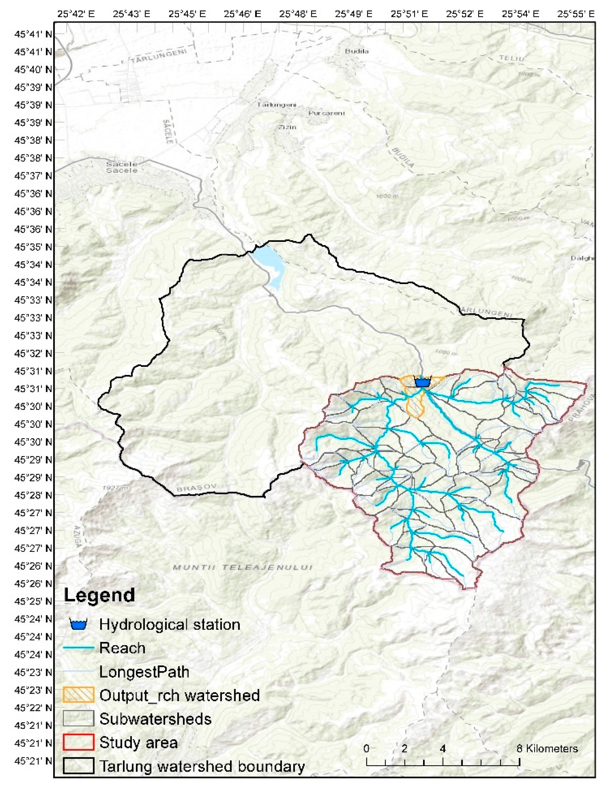
Figure 1. Upper Tarlung watershed.
Water 14 02860 g001
Figure 2. Land use (AGRL—Agricultural land; FRSD—Forest deciduous; FRSE—Forest evergreen; PAST—Mountain meadow; RNGB—Pasture with trees; RNGE—Meadows; SWRN—Rocky lands; URML—Built-up areas; UTRN—Roads; WATR—Water body) categories distribution within the Upper Tarlung watershed.
Water 14 02860 g002
Figure 3. Soil types (REND—Rendoll; EUTRT—Eutric cambisols typic; EUTRM—Eutric cambisols mollic; EUTRL—Eutric cambisols lithic; EUTRG—Eutric cambisols gleyc; EUTRS—Eutric cambisols stagnic; DYSTT—Dystric cambosols typic; DYSTU—Dystric cambosols umbric; DYSTL—Dystric cambosols lithic; HAPLL—Prepodzol lithic; HALPH—Prepodzol histic; UDORL—Litosol; DYSTRFL—Aluviosols dystric; DYSTRFLG—Aluviosols gleyic) distribution within the Upper Tarlung watershed.
Water 14 02860 g003
Figure 4. Flow chart of the methodology used in this study.
Water 14 02860 g004
Figure 5. Graphical result of the sensitivity analysis.
Water 14 02860 g005
Figure 6. Changes in temperature as percentual differences compared with baseline for: (a) short, (b) mid, and (c) long term.
Water 14 02860 g006
Figure 7. Changes in precipitation as percentual differences compared with baseline for: (a) short, (b) mid, and (c) long term.
Water 14 02860 g007
Figure 8. Seasonal surface runoff (%) projected for 2020–2039 in: (a) REMO4.5, (b) CLM4.5, (c) REMO8.5, and (d) CLM8.5.
Water 14 02860 g008
Figure 9. Seasonal surface runoff (%) projected for 2040–2069 in: (a) REMO4.5, (b) CLM4.5, (c) REMO8.5, and (d) CLM8.5.
Water 14 02860 g009
Figure 10. Seasonal surface runoff (%) projected for 2070–2100 in: (a) REMO4.5, (b) CLM4.5, (c) REMO8.5, and (d) CLM8.5.
Water 14 02860 g010
Table 1. Description of the scenarios used in the simulation.
Adopted ScenarioClimate ChangeCurrent Land UseLand Use Change
by 25%
Land Use Change
by 50%
Scenario 1
Scenario 2
Scenario 3
Table 2. Parameters used in the calibration.
ParameterDescriptionVariation IntervalFitted Value
MinimumMaximum
V__REVAPMN.gwThreshold depth of water in the shallow aquifer for revap or percolation0.000000500.000000134.500000
R__OV_N.hruManning’s “n” value for overland flow−0.2000000.000000−0.128600
R__HRU_SLP.hruAverage slope steepness0.0000001.0000000.613000
R__SOL_K(..).solSaturated hydraulic conductivity−0.8000000.800000−0.776000
R__SOL_AWC(..).solAvailable water capacity of the soil layer−0.2000000.100000−0.119900
V__GW_REVAP.gwGroundwater “revap” coefficient0.0200000.2000000.025580
R__SOL_BD(..).solMoist bulk density−0.5000000.6000000.312900
V__ESCO.hruSoil evaporation compensation factor0.0000001.0000000.699000
V__LAT_TTIME.hruLateral flow travel time0.000000180.0000005.940000
R__CN2.mgtSCS runoff curve number−0.2000000.200000−0.016400
V__ALPHA_BF.gwBaseflow alpha factor0.0000001.0000000.931000
V__GWQMN.gwThreshold depth of water in the shallow aquifer for return flow0.0000005000.00000075.000000
Table 3. Testing influence of climate change scenarios on surface runoff.
Climate ScenariosREMO4.5REMO8.5CLM4.5CLM8.5
Mean surface runoff
(thousand cm)
979 a930 ab933 a903 a
Significant differences are indicated by different letters, and insignificant differences are indicated by the same letters at p < 0.05.
Table 4. Testing influence of land use change scenarios on surface runoff.
Land Use ScenariosS1S2S3
Mean surface runoff
(thousand cm)
870 a932 ab1006 b
Significant differences are indicated by different letters, and insignificant differences are indicated by the same letters at p < 0.05.
Table 5. Testing influence of season on surface runoff.
SeasonWinter Spring SummerAutumn
Mean surface runoff
(thousand cm)
1178 a1197 b249 c319 c
Significant differences are indicated by different letters, and insignificant differences are indicated by the same letters at p < 0.05.
Publisher’s Note: MDPI stays neutral with regard to jurisdictional claims in published maps and institutional affiliations.