Article

The Use of GAMLSS Framework for a Non-Stationary Frequency Analysis of Annual Runoff Data over a Mediterranean Area

Dipartimento di Ingegneria, Università degli Studi di Palermo, 90128 Palermo, Italy
*
Author to whom correspondence should be addressed.
Water 2022, 14(18), 2848; https://doi.org/10.3390/w14182848
Submission received: 4 August 2022 / Revised: 2 September 2022 / Accepted: 8 September 2022 / Published: 13 September 2022
(This article belongs to the Section Hydrology)

Abstract

:
Climate change affects all the components of the hydrological cycle. Starting from precipitation distribution, climate alterations have direct effects on both surface water and groundwater in terms of their quantity and quality. These effects lead to modifications in water availability for agriculture, ecology and other social uses. Change in rainfall patterns also affects the runoff of natural rivers. For this reason, studying runoff data according to classical hydrological approaches, i.e., statistical inference methods that exploit stationary probability distributions, might result in missing important information relevant to climate change. From this point of view, a new approach has to be found in the study of this type of data that allows for non-stationary analysis. In this study, the statistical framework known as Generalized Additive Models for Location, Scale and Shape (GAMLSS), which can be used to carry out non-stationary statistical analyses, was applied in a non-stationary frequency analysis of runoff data collected by four gauges widely distributed across Sicily (Italy) in the period 1916–1998. A classical stationary frequency analysis of these runoff data was followed by a different non-stationary frequency analysis; while the first was made using annual rainfall as a covariate, with the aim of understanding how certain statistical parameters of runoff distribution vary with changes in rainfall, the second derived information about the temporal variability of runoff frequencies by considering time as a covariate. A comparison between stationary and non-stationary approaches was carried out using the Akaike information criterion as a performance metric. After analyzing four different probability distributions, the non-stationary model with annual rainfall as a covariate was found to be the best among all those examined, and the three-parameter lognormal the most frequently preferred distribution.

1. Introduction

Runoff frequency analysis is fundamental to the development of methods for the statistical estimation of quantiles based on observed data. Such methods are widely used in the development of specific rules concerning water resource management and in the generation of synthetic runoff time series for ungauged basins [1].
The scientific literature does not contain many studies on probability distributions for annual runoff. One of the first approaches has been provided by Markovic [2], who investigated the goodness of fit of probability distributions of annual runoff in Western USA and southwestern Canada using the chi-squared statistic. The results of the work showed that all five probability functions taken into account (normal, two-parameter lognormal, three-parameter lognormal, two-parameter gamma and three-parameter gamma) were applicable and that no distribution could be preferred to the others in fitting an observed single-station sample of annual river flow distributions. In particular, the differences in goodness of fit in ensemble analyses between the two-parameter lognormal and two-parameter gamma distributions can be considered, for practical purposes, negligible. Therefore, in the analysis of larger-scale distributions, these two functions are interchangeable.
Later, Vogel et al. [3] investigated probability distributions for annual maximum, mean and minimum streamflows at more than 1455 river basins in the USA, with record lengths ranging from 6 to 115 years and with an average of 45.5 years of records per site, using L-moment diagrams to measure the goodness of fit between the sample data and the selected probability distributions. The authors highlighted that, among all the two-parameter distributions taken into account (gamma and two-parameter lognormal), the gamma (GAM) distribution was the one that captured the observed relationships between the L-moments L-CV and L-Skew of average annual flows in the United States. However, the results also showed that the three-parameter Pearson (P3), three-parameter lognormal (LN3) and three-parameter log Pearson (LP3) distributions provided better approximations to the observed L-moment relationships for average annual flows than any two-parameter distribution considered. Given the theoretical justification provided for the gamma and P3 distributions, the authors recommended the use of either of these likelihood functions to model average annual flows in the USA.
In contrast, Cannarozzo et al. [1] performed a frequency analysis of annual runoff data recorded in Sicily (Italy) by identifying homogeneous regions and fitting, for each region, a single probability distribution function to the annual runoff data, scaled by the index runoff (the mean annual runoff). The authors used the chi-square test for goodness-of-fit testing. The advantage of using this procedure was that both the frequency growth curve and the runoff index could be estimated using morphological and climatic characteristics of the watersheds easily identified in a GIS environment, such as average annual rainfall, average elevation and average slope of the watershed.
Due to changes in climate and basin characteristics, the statistics of annual runoff series show complex and non-stationary changes. For this reason, the assumption that the distributions in a frequency analysis of hydrological variables will be in equilibrium around an underlying mean and that the variance will remain constant over time can be questioned.
The design of different hydraulic infrastructures and the management of water supply systems, irrigation systems and hydropower are usually based on conventional frequency analyses, which estimate the statistics for a time series of a certain hydrological variable by assuming the stationarity of the recorded series, i.e., they are “devoid of trends, shifts or periodicity (cyclicity)” [4]. Historically, in fact, statistical inference in hydrology has relied heavily on this assumption, such that the distribution of the variable of interest has been considered invariant with respect to time.
Generally, however, in a changing environment, combinations of multiple factors, such as precipitation, temperature, evapotranspiration and, for example, reservoir construction, can lead to variations in flow regimes by altering flow characteristics, i.e., the seasonality of runoff and the frequency and magnitude of floods [5]. In fact, stream runoff has shown significant changes globally due to the impact of climate change, mainly because of anthropogenic effects on climate and basin characteristics [6,7,8]. For this reason, methods that account for non-stationarity have been developed in order to replace long-established characteristic principles of estimation of distribution parameters and, consequently, water resource management and to shift to an evolutionary paradigm. Such a paradigm must recognize the dynamics of physical and socio-economic processes [9]. Several studies have, therefore, introduced the concept of hydrological non-stationarity in the analysis of various hydrological variables and, beyond this, have demonstrated that the stationary method is no longer reliable [10,11,12,13,14,15,16].
Although, today, many still debate whether stationarity is immortal [17], alive [18] or dead [19], it is well known that human activities and climate change have significant impacts on runoff and other hydrological processes [8,20,21,22,23,24]. The current literature on frequency analysis of non-stationary hydrological variables focuses mainly on two issues: (i) the development of the non-stationary method and (ii) the exploration of covariates that reflect changes in hydrological variables. Many studies [7,25,26] have presented the time-varying moment method, which assumes that the hydrological variable of interest follows a certain type of probability distribution, whose moments change over time [27].
The choice of probability distribution is also of paramount importance. Frequency analysis using distributions that poorly match the sample under examination can lead to errors in the evaluation and estimation of hydrological variables. The basic idea is, therefore, to assume that the type of distribution for the analyzed hydrological variable is unchanging, while its statistical parameters may change over time or with other covariates. In Villarini et al. [28], this method was presented using Generalized Additive Models for Location, Scale and Shape parameters (GAMLSS; [29]) as a flexible framework for evaluating non-stationary time series, using time as a covariate. The time-varying parameter method can be extended to the analysis of physical covariates, such as precipitation, by replacing time with any other physical time-dependent covariate [30,31,32,33]. The covariate approach incorporates covariates into the parameters of distributions because the dependence of model parameters on covariates is useful for representing the dependence of hydrological time series on slowly varying climate forcing.
For example, Li et al. [34] conducted a non-stationary runoff frequency analysis for future climate changes and studied the relevant uncertainties. The main purpose of this study was to analyze the non-stationarity of runoff frequencies adjusted for future climate change in the Luanhe River Basin, China. Non-stationary GAMLSS models were established for the analysis of the non-stationary frequency of runoff (1961–2010), using observed rainfall as a covariate, which is closely related to runoff and contributed significantly to its non-stationarity. The results showed that the sources of uncertainty in the statistical parameters of the non-stationary model arise mainly from fluctuations in the precipitation sequence. This result indicates the need to consider the precipitation sequence as a covariate in runoff frequency analysis in the future.
The objective of our study was, therefore, to investigate the non-stationarity of annual runoff through a non-stationary frequency analysis for some Sicilian rivers, considering the dependence of this variable on time and annual rainfall, which were here used as covariates. The GAMLSS method was applied for the analysis of stationary and non-stationary runoff frequencies. First, the stationary frequency analysis was performed, followed by the non-stationary frequency analysis and a comparison of the two methodologies. The non-stationary analysis was carried out by considering rain as a covariate, which, in turn, showed non-stationary characteristics. Secondly, through a non-stationary analysis with time used as a covariate, information on the temporal variability of the runoff distribution parameters was derived.
Through these approaches, different probability distributions commonly used in similar cases were taken into account in trying to identify the one that best fitted the relevant dataset. The annual runoff data studied were provided by four gauges managed by Autorità di Bacino of the Regione Siciliana (AdB).
The paper is structured as follows: following this introduction is a section on materials and methods; the third section describes and discusses the achieved results; and, finally, the last section presents the conclusions of the study.

2. Materials and Methods
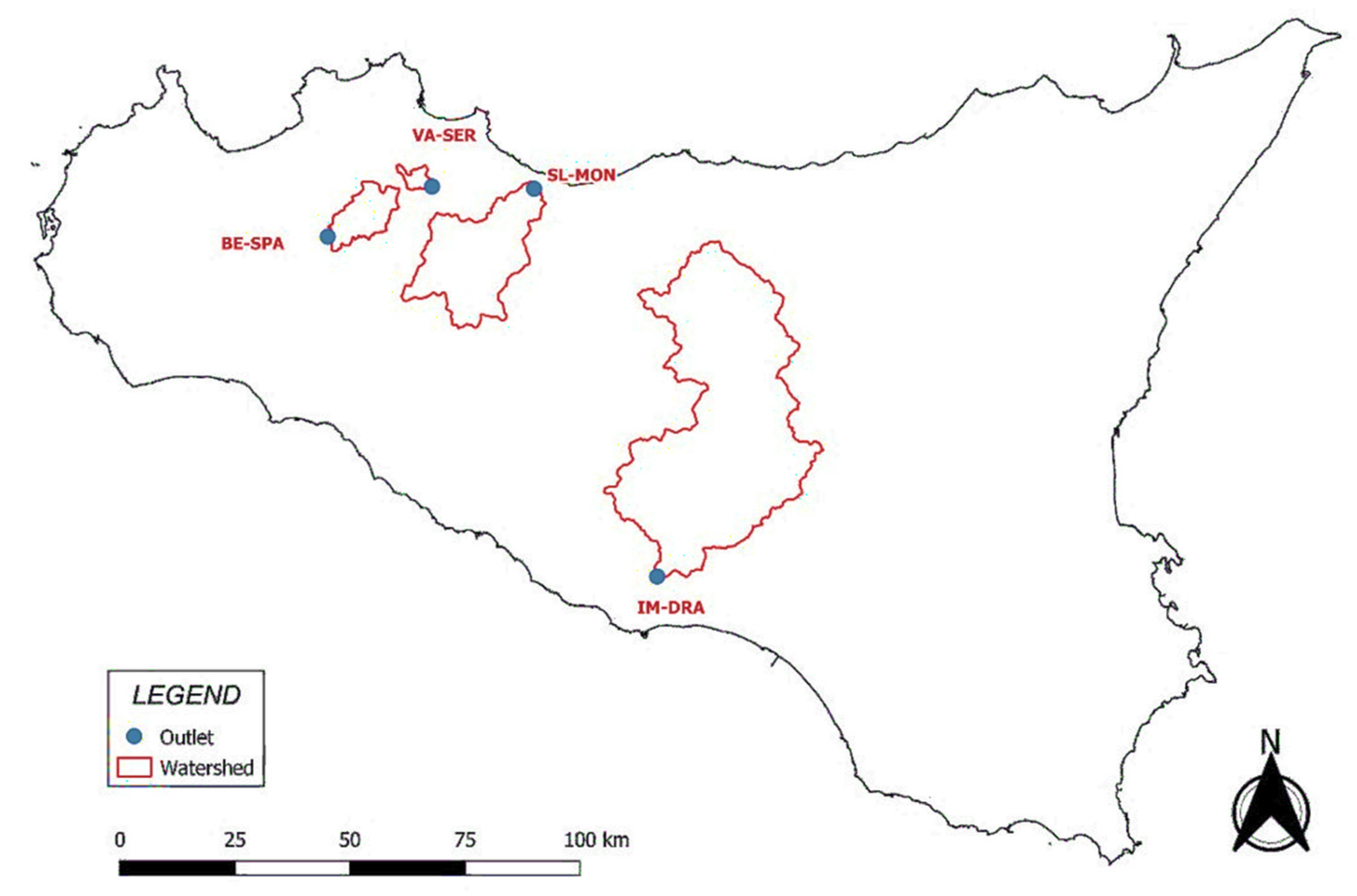
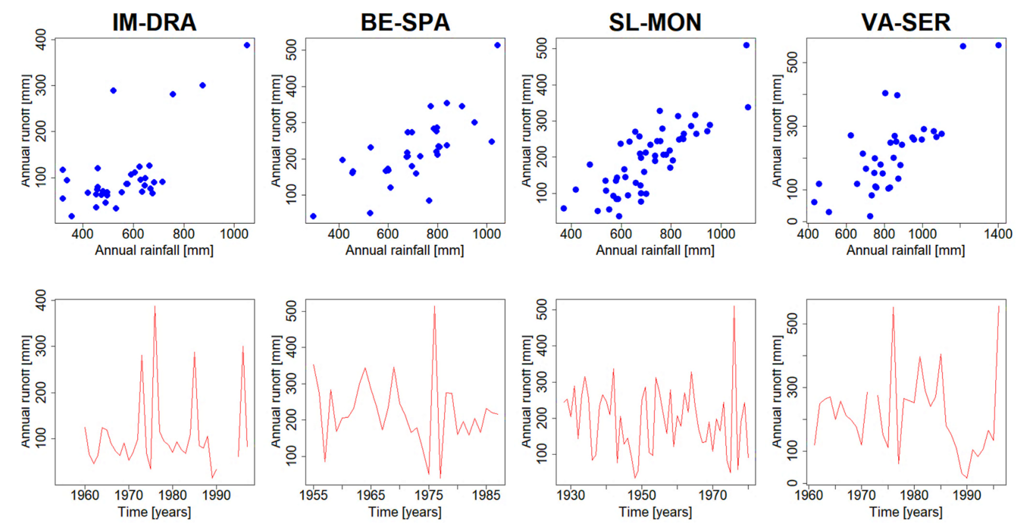
This section presents the data used in this study along with the adopted methodology. The GAMLSS framework is described, and the adopted statistical distributions are also presented. In addition, the Akaike information criterion (AIC), used for testing the goodness of fit of the various statistical distributions and models, is described. For the sake of clarity, Figure 1 displays a flow chart of the adopted methodology.

2.1. Data

The data used in this study were provided by the Autorità di Bacino of the Regione Siciliana. The gauge stations analyzed were those at the outlets of the watersheds “Belice river at Sparacia” (hereinafter named BE-SPA), “Imera river at Drasi” (IM-DRA), “San Leonardo river at Monumentale” (SL-MON) and “Valle dell’Acqua river at Serena” (VA-SER). For each station, annual rainfall and runoff time series (averaged over the watershed) were collected. These stations were chosen among different gauges used by Cannarozzo et al. [1] because they had the largest sample sizes. In addition, these gauge stations were selected because their runoff time series exhibited different behaviors. The use of various statistical tests highlighted the presence of a trend in BE-SPA, SL-MON and VA-SER annual runoff time series, while heteroscedastic behavior for annual runoff vs. time was found for IM-DRA and VA-SER. This suggested the use of a non-stationary statistical approach to deal with the annual runoff time series of these gauge stations.
The working periods of three measurement sites began in the late 1950s or early 1960s while that for SL-MON, which had the largest sample size, began in the late 1920s.
In particular, the sample sizes were equal to 33, 34, 53 and 35 values for BE-SPA, IM-DRA, SL-MON and VA-SER, respectively. The geographical locations of the considered stations, located at the outlets of the related catchments, are shown in Figure 2, while Figure 3 shows scatterplots of runoff (q) vs. rainfall (p) and vs. time (t) for each gauge.

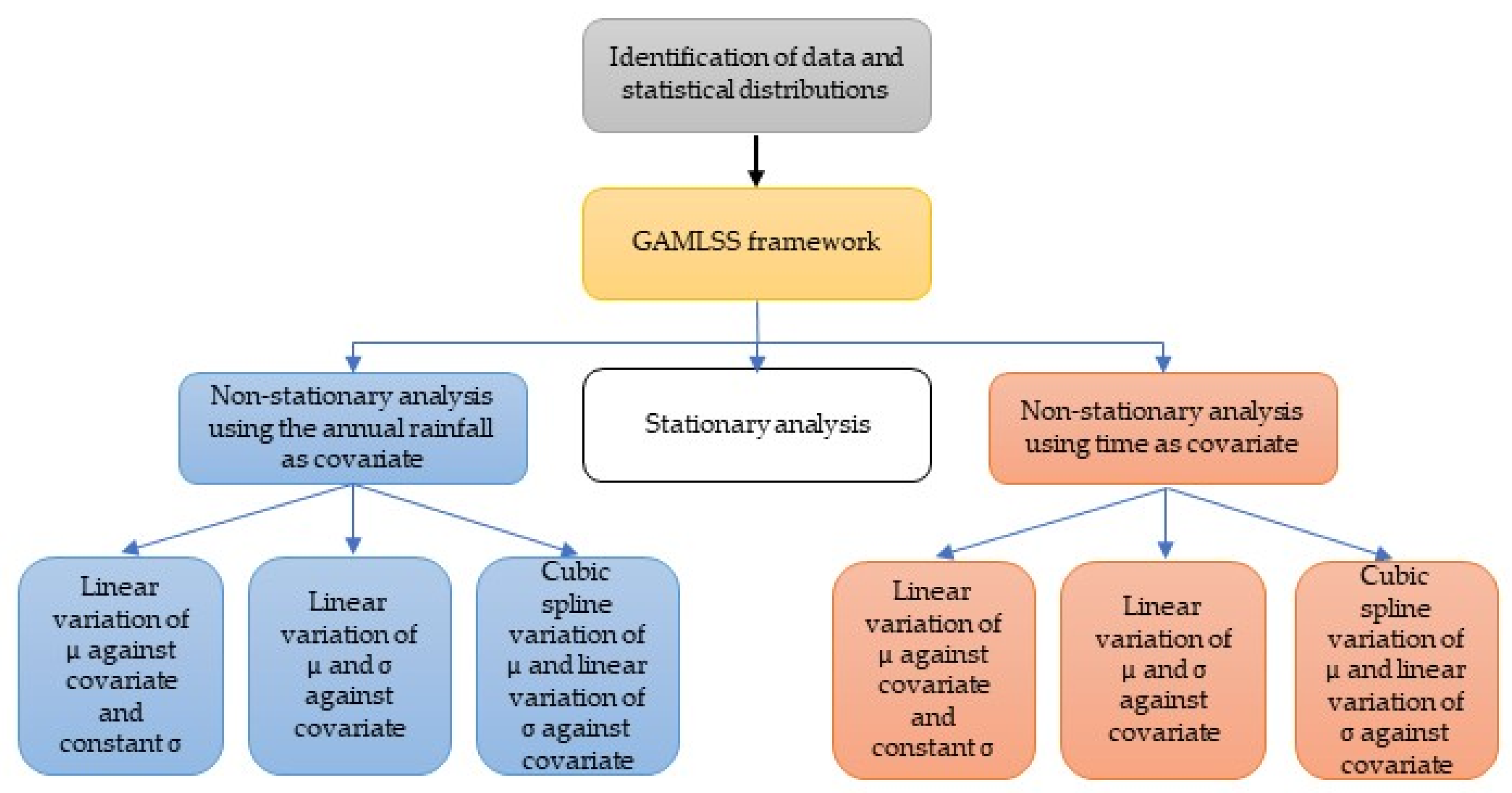
2.2. The Generalized Additive Models in Location, Scale and Shape (GAMLSS) Framework

In this study, a general class of regression models, widely known as Generalized Additive Models in Location, Scale and Shape (GAMLSS), was adopted to carry out the stationary and non-stationary runoff frequency analyses.
In GAMLSS, the exponential family distribution assumption for the response variable y is relaxed and replaced by a general distribution family, including highly skewed and/or kurtotic distributions. The systematic part of the model is extended to allow modeling not only of the mean but also of the other parameters of the distribution. This can be carried out by means of linear parametric and/or additive non-parametric functions of explanatory variables and/or random effects. Maximum likelihood estimation is used to fit the models.
GAMLSS can be defined as semi-parametric regression models. These models are “parametric”, since they require parametric distribution assumptions for the response variables, and “semi-” in the sense that modeling of the distribution parameters, as functions of the explanatory variables, may involve non-parametric smoothing functions.
A GAMLSS model assumes that a certain number of independent observations, yi, for i = 1, 2, …, n, are distributed according to a probability density function, f(yii), conditional on θi = (θ1i, θ2i, θ3i, θ4i) = (µi, σi, νi, τi), which represents the ensemble of four distribution parameters, each of which can be a function of the explanatory variables.
For this reason, hereafter, we refer to (µi, σi, νi, τi) as the distribution parameters. The first two of them, µi and σi, are usually mentioned as location and scale parameters, while the remaining parameter(s), if any, are characterized as shape parameters, e.g., skewness and kurtosis parameters.
In any case, the regression model may be applied more generally to the parameters of any population distribution and can be generalized to more than four distribution parameters. Rigby and Stasinopoulos [29] introduced the original formulation of a GAMLSS model. One can consider y′ = (y1, y2, …, yn) the n-length vector of the response variable and let gk(·) (for k = 1, 2, 3, 4) be the monotonic functions linking the distribution parameters to the explanatory variables:
g 1 ( μ ) =   η 1 = X 1 β 1 + j = 1 J 1 h j 1 ( x j 1 )
g 2 ( σ ) =   η 2 = X 2 β 2 + j = 1 J 2 h j 2 ( x j 2 )
g 3 ( ν ) =   η 3 = X 3 β 3 + j = 1 J 3 h j 3 ( x j 3 )
g 4 ( τ ) =   η 4 = X 4 β 4 + j = 1 J 4 h j 4 ( x j 4 )
where µ, σ, ν, τ and ηk and xjk, (for j = 1, 2, …, Jk) and k = 1, 2, 3, 4 are vectors of length n. In many practical situations, four distribution parameters are required at most. The function hjk is a non-parametric additive function of the explanatory variable Xjk evaluated at xjk. The explanatory vectors xjk are assumed to be fixed and known. In addition, Xk, for k = 1, 2, 3, 4, are fixed design matrices (fixed effects design matrices of explanatory variables, i.e., covariates) while βk are the vectors of the parameters of the distribution. Usually, in typical applications, a constant or other simple model is often suitable for each of the two shape parameters (ν and τ).
The above model is called the semi-parametric GAMLSS model and has been extended to allow random effect terms to be included in the model for µ, σ, ν and τ [29].
The parametric vectors βk and k = 1, 2, 3, 4 are estimated within the GAMLSS framework by maximizing a penalized likelihood function.
The GAMLSS framework implemented in the R package (used for the presented analyses) allows for the fast fitting of different models (i.e., linear or non-linear dependence of means with respect to covariates) to a dataset. The selection of the model that best suits the data can be performed by checking the significance of the fitting improvement, e.g., between stationary and non-stationary models, by means of deviance statistics.

2.3. Statistical Distributions in GAMLSS

According to the properties of the analyzed dataset, the theoretical distribution functions that best fitted the observed annual rainfall and runoff data had to reflect the following characteristics: (i) the function had to be continuous and defined for positive values of the variable, (ii) the lower tail had to be bound by zero or a positive value, (iii) the upper tail had to be unbounded, (iv) the density curve had to be asymptotic to the axis for large values of the analyzed variable, (v) the basic shape had to be a two-tailed bell curve with a wide variety of skewness, and, lastly, (vi) the number of parameters describing the theoretical functions had to be limited to three.
The choice of various probability distributions was based on the analysis of the types of best-fit probability functions for annual precipitation and runoff distributions reported by Markovic [2], in which the following distribution types were studied: normal distribution (NO), two parameter log-normal distribution (LOGNO), three-parameter log-normal distribution (LNO) and two-parameter gamma distribution (GA) [3]. The LNO distribution, as reported by Stasinopoulos et al. [35], is a two-parameter fit for µ and σ, while ν is fixed.
The equations for the chosen distributions with the related moments are shown below, in Table 1.

2.4. The AIC Criterion

The evaluation of the goodness of fit for the above-mentioned distributions to each runoff dataset was carried out using the Akaike information criterion [36], here referred to as AIC, which is a method for evaluating and comparing statistical models. It provides a measure of the estimation quality of a statistical model by taking into account both the goodness of fit and the complexity of the model. AIC is calculated from:
1.
The number of independent variables used to build the model;
2.
The maximum likelihood estimates of the model.
In the general case, the AIC is defined as:
AIC = 2 k 2   ln ( L )
where k is the number of parameters in the model and L is the maximum value of the likelihood function for the model. The default k is 2, so a model with one parameter will have a k of 2 + 1 = 3. In general, the model that best fits the data is the one with the lowest AIC. If a model is more than 2 AIC units lower than another, then it is considered significantly better than that model. In the analysis of time series, it is common to try some kind of transformation on the variable [37]. The decision about the choice of the transformation can be simply realized by using the likelihoods of the models. The effect of transforming the variable is represented by the product of the likelihood and the corresponding Jacobian, and thus by the addition of minus twice the logarithm of the Jacobian to the AIC. In the case of log {y(n)}, it is 2 ∑log {y(n)}, where the summation extends over n = 1, 2, …, N and N is the length of the data. The correct AICs are obtained after these corrections for the Jacobians.

3. Results and Discussion

This section presents the results obtained by applying GAMLSS to the rainfall–runoff data collected at the examined stations. Section 3.1 is devoted to the stationary frequency analysis, while the other two sections discuss the non-stationary frequency analysis considering rainfall (Section 3.2) and time (Section 3.3) as covariates. The non-stationary analysis for both covariates was performed following three different combinations: (i) linear dependence of μ with respect to the covariate under consideration and constant σ, (ii) linear dependence of μ and σ with respect to the covariate under consideration and (iii) fitting of a non-parametric smoothing model for μ and a linear σ dependence, again with respect to the same covariates.

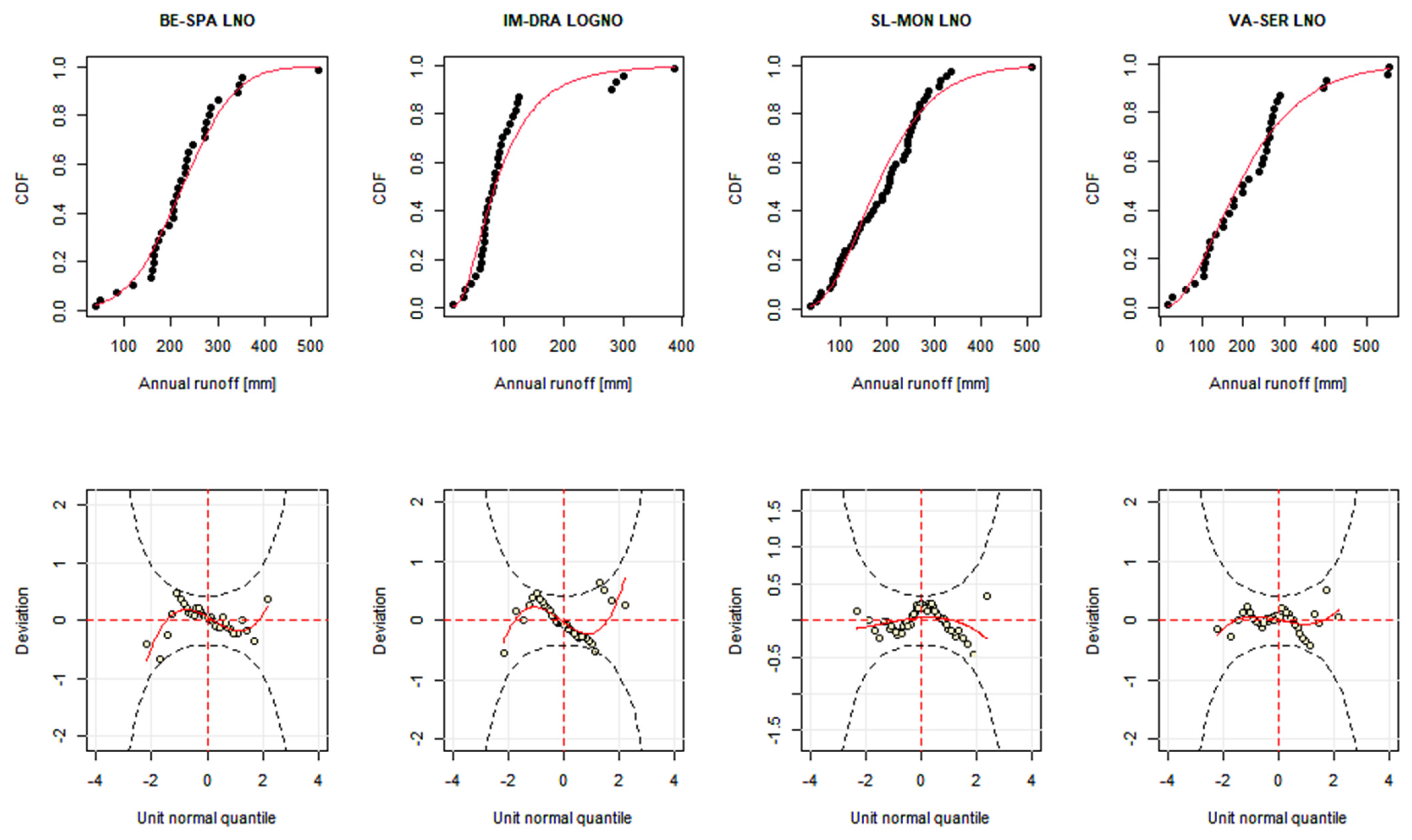
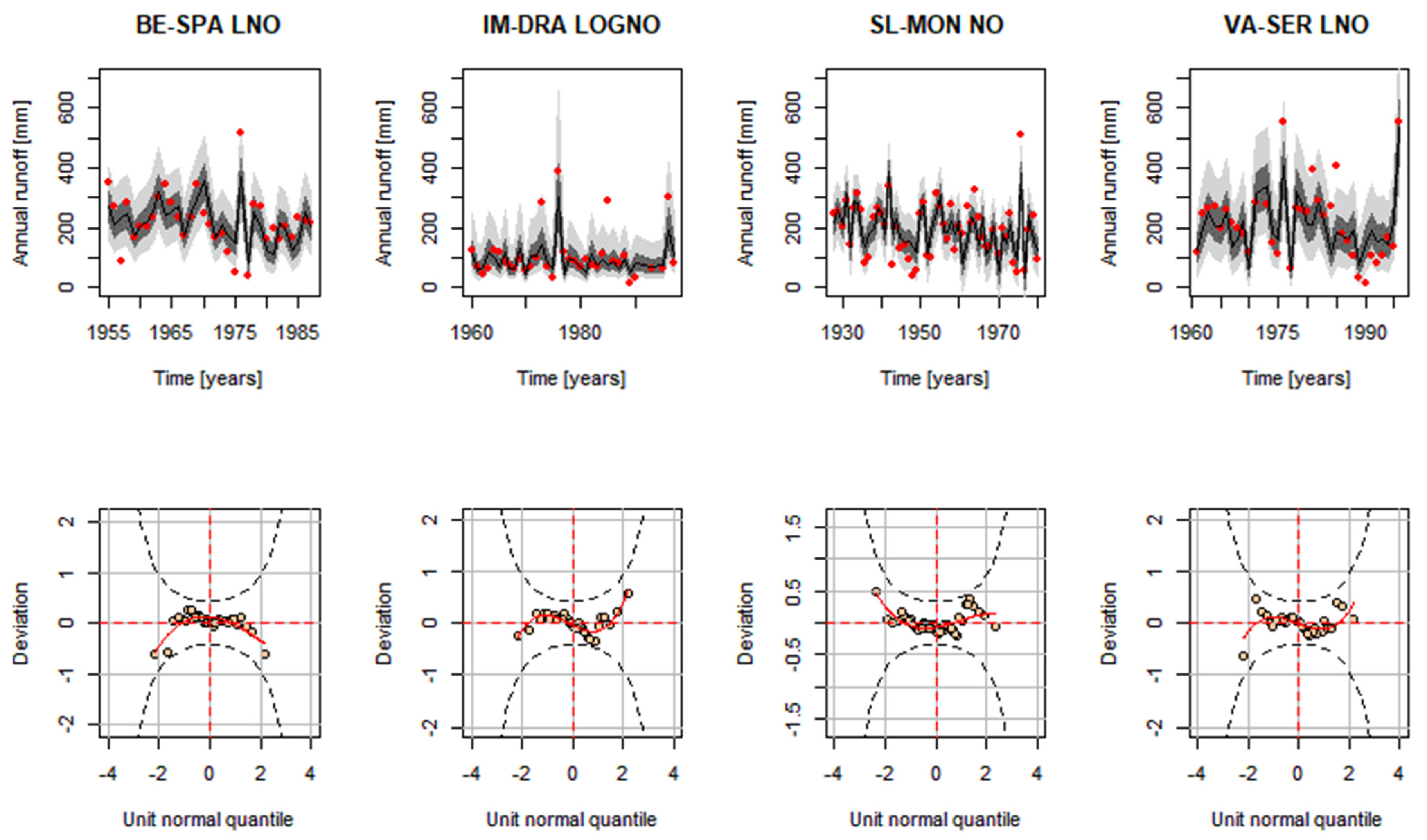
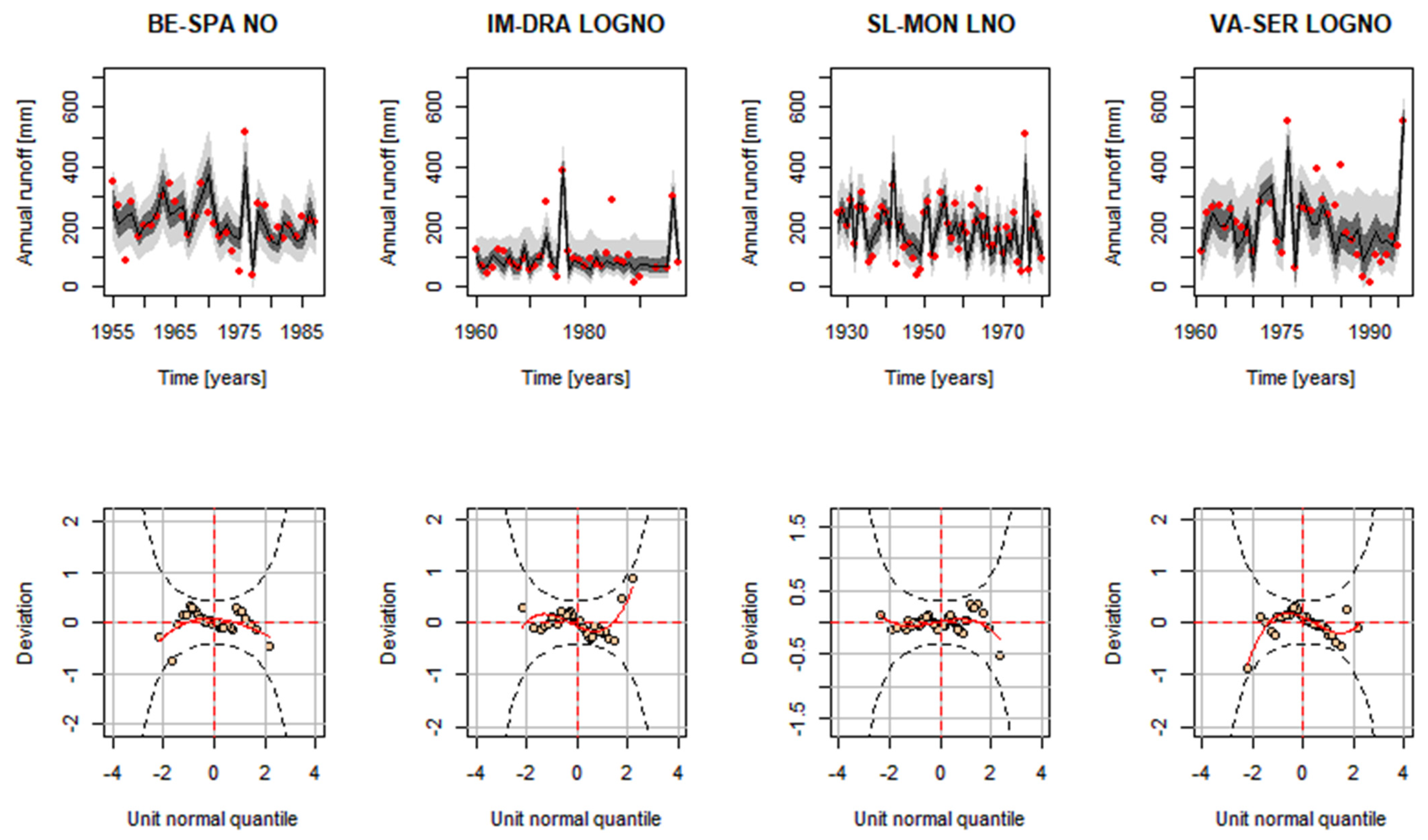
3.1. Stationary Analysis

Nelson [38] provided a statistical definition of stationarity, stating that it means that the statistical parameters of a data series computed from different samples do not change except due to sampling variations.
Shumway and Stoffer [39] distinguish between two orders of stationarity, making a distinction between strictly stationary and weakly stationary time series. A time series is said to be strictly stationary if its statistical properties do not vary over time. In other words, if a time series has a constant mean and variance, it is a stationary time series. A less strict type of stationarity, known as weak or second-order stationarity, is one in which first- and second-order moments depend only on temporal differences [40]. Essentially, the length that time series can be observed is limited, as in the case of hydrological time series. Therefore, weakly stationary time series are practically treated as stationary time series. A stationary time series cannot have any trend or periodic component. Conversely, if a series does not have a constant mean or variance, it is not stationary.
In order to study the classical approach to the stationary analysis of runoff data, the above-mentioned distributions (Table 1) were applied and then compared.
For data from all the gauges considered, the log transformation provided better AIC values. In particular, for IM-DRA, the best distribution was the LOGNO distribution, while for three gauge sites the best distribution, in terms of AIC, was LNO. Where the behavior of the runoff data was visibly far from that of a normal distribution, the optimal AIC value greatly differed from the AIC of the NO distribution (i.e., IM-DRA). The distributions that best fitted the samples under investigation are shown in Table 2, with the respective AIC values highlighted in bold, and in Figure 4.
In particular, the first row in Figure 4 represents the empirical (points) and theoretical (red line) cumulative distribution functions (cdfs) for the adopted distributions for the four gauge stations.
The second row shows the relatives worm plots of the best distributions provided by the AIC test. The worm plot [41] is a diagnostic tool for checking the residuals within different ranges of the explanatory variables, with elliptical curves indicating approximate 95% point-wise confidence bands. Ideally, the points in the worm plot should be close to the horizontal line in the middle with no systematic shape and 95% or more of the points inside the elliptical curve [42]. With worm plots, it is thus possible to visualize the differences between different distributions, conditioned on the values of a covariate. The quadratic and cubic shapes of the residuals in worm plots highlight that the empirical skewness and kurtosis have not been appropriately captured by the chosen distribution model, even if the models are characterized by low AIC values. Particularly for IM-DRA and SL-MON, not all points fell within the confidence band. A cubic trend for the residuals can be observed for BE-SPA, IM-DRA and VA-SER. For SL-MON, on the other hand, the trend of the residuals is characterized by a quadratic shape.

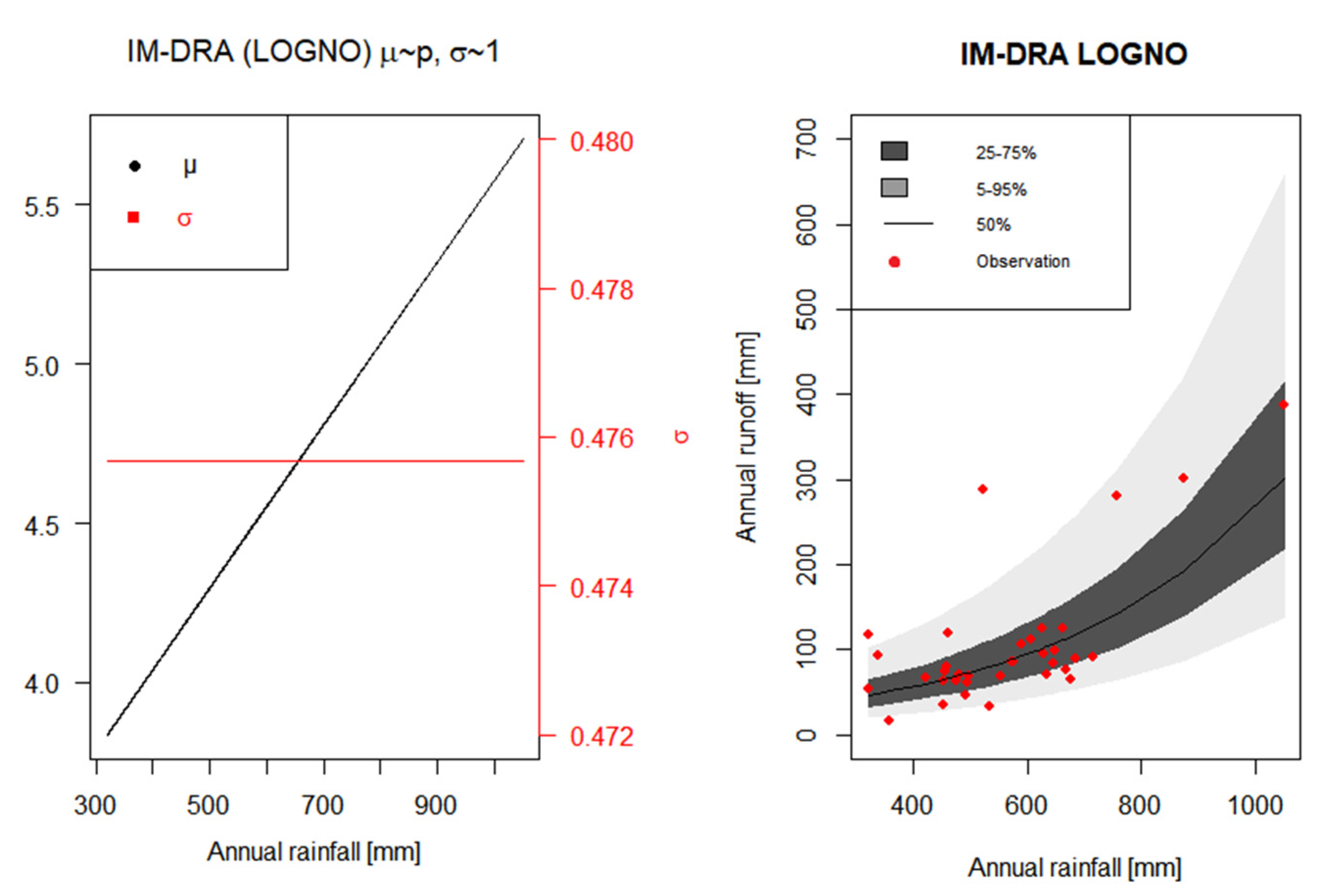
3.2. Non-Stationary Analysis with Rainfall as a Covariate

In this section, the application of a non-stationary analysis is presented. In the first step, a linear dependence of the location parameter µ with annual rainfall was imposed. The scale parameter σ was constant (µ~p, σ~c, where “~c” means that the µ/σ parameter was constant and “~p” means that the µ/σ parameter was modelled as a linear function of annual rainfall). Hereinafter, this is referred to as the P1 model. In the parameter estimation for the GAMLSS framework, the algorithm proposed by Rigby and Stasinopoulos [43] and Rigby and Stasinopoulos [44] was used to calculate the parameters of the optimal model, with the maximum penalized likelihood function as the objective function. Through this analysis, it was possible to derive plots which showed trends for μ and σ with respect to the covariate.
For example, considering the P1 model, the distribution best fitting the IM-DRA data was the LOGNO. In this case, imposing the linear variation of the µ parameter with rainfall and keeping the value of σ constant (so that it did not depend on annual rainfall) resulted in an increasing pattern of µ and a constant pattern for σ (left panel of Figure 5) with respect to rainfall. These patterns of µ and σ resulted in nonlinear behavior of the median and the variability of the distribution with rainfall, as in the centiles plot shown in the right panel of Figure 5. There, the black line represents the 50th percentile curves (i.e., median), the dark-gray regions represent the areas within the 25–75% centile curves, the light-gray regions represent the areas within the 5–95% centile curves and the red dots in the centiles plot represent the observed runoff data.
For the P1 model, the variation of the dependent variable (the runoff) was itself not automatically linear, since this actually depended on the type of distribution. Looking at the moments’ equations related to the LOGNO distribution in Table 1, the linear variation of µ reflects an exponential growth of both the first two moments (mean and variance). This, in turn, leads to a nonlinear increase in the location and shape of the distribution and, hence, to a progressively nonlinear widening of the centile curves as annual rainfall increases. Only in the case of the NO distribution will the trend of the median with rainfall and the variability of the distribution be linear.
For the P1 model, the best distributions, according to the AIC, were the LNO for the BE-SPA and VA-SER sites, the LOGNO for the IM-DRA site and the NO distribution for the SL-MON gauge site. Goodness of fit for the models was assessed using centile curve diagnostic plots and worm plots [41].
Figure 6 shows the centile curves and worm plots of the best distributions for each site. In the first row of Figure 6, the centiles plot highlights how, year by year, the probability distributions adopted change as a function of the rainfall covariate. The variability of the distribution, which does not always remain constant, changes according to the parameters of the distribution itself; in fact, the location parameter varies linearly with annual rainfall, while, as mentioned above, σ is kept constant for each value of the covariate.
Moreover, most of the red points are within the 5% and 95% curves for the optimal models, indicating that the models describe the variability of the observed data reasonably well. The percentage of the number of points outside the 5–95% centile band is always less than 10% of each station’s sample size and equal to 6%, 6%, 9% and 9% for BE-SPA, IM-DRA, SL-MON and VA-SER, respectively.
The panels in the second row of Figure 6 show that the points of the optimal models are all within the 95% confidence intervals, indicating that the residuals are approximately normally distributed. Just as with the stationary analysis, the distributions chosen through the AIC still show the residuals with quadratic and cubic shapes in the worm plots. In this case, an improvement in the goodness of results, shown through the worm plots, and a decrease in the AIC values as compared to the S-model make it clear that the modeling of the location parameter with an external covariate has a considerable impact on this type of non-stationary analysis.
Since a nonlinear pattern was noticed in the variability of the probability distributions, which in addition to the µ parameter is certainly related to the σ parameter, a further analysis was carried out by introducing, in addition to the linear variation of µ with rainfall, that of σ with annual rainfall as covariate (µ~p, σ~p—P2).
The introduction of a linear modeling of the σ parameter with rainfall improved the description of the runoff probability distributions for all four watersheds. In this case, the distributions with the lowest AIC values, which therefore minimized the likelihood functions, were the NO distribution for the BE-SPA site, the LOGNO distribution for the IM-DRA site and the LNO distribution for the SL-MON and VA-SER sites.
Thus, the best distributions in terms of AIC values did not remain unchanged for BE-SPA and SL-MON compared with the previous model. In Figure 7, it can be seen how the linear modeling of σ leads to a change in the shape of the centile curves with respect to the former analysis. In fact, this new modeling approach resulted in a thinning of the bands in the centiles plots, especially the 75th to 95th percentile bands suggesting that, compared with the previous model, the variability of the distributions for the highest centile values decreased. Even in this case, the behavior of the centile curves against annual rainfall (not shown in the plot) was no longer perfectly linear, as reported in Zhang et al. [45]. The NO distribution (the best-fitting distribution for the BE-SPA site), for which the second-order moment was governed by the square σ, also showed a nonlinear pattern compared with the previous model.
In this case, the P2 model is more suitable than the previous one for capturing changes in the variability of distributions with rainfall for all gauge sites, and this is also attested by a decrease in AIC values for all the four sites. For all the gauge sites, the trend of residuals within the 95% confidence interval of worm plots underwent considerable flattening (Figure 7), which is diagnostic of an improvement compared with the previous analysis.
As already reported, a decrease in AIC means an improvement in model performance. This was more evident for the P1 model than in the case (not shown in this paper) in which only σ was linearly modeled as a function of rainfall. For this reason, a more in-depth modeling of the µ parameter was explored. In particular, a further analysis was carried out with a higher degree of complexity, in which the location parameter, μ, was considered as a non-parametric smoothing cubic-spline function of the covariate rainfall with three effective degrees of freedom; the linear modeling of the parameter σ with the rainfall covariate was maintained (µ~cs(p), σ~p—P3). “~cs(p)” means that the µ/σ parameter was modelled as a cubic spline of annual rainfall.
At this stage, the best distributions remained unchanged when compared with the previous analysis, the only exception being the VA-SER site. Centile curves for all stations and the related worm plots are shown in Figure 8. What is interesting to point out is that there is a thinning of the 5–25% centile curve ranges, a widening of the 75–95% ones and a lowering of the black (median) line, particularly for the IM-DRA and VA-SER sites. The 25–75% bands, on the other hand, also tend to follow the points characterized by high runoff values in greater detail. In relation to this model, the worm plots always show good distributions of residuals, with all points within the 95% confidence interval, but also quadratic or cubic trend lines that are more evident than in the previous analyses. This is, indeed, reflected in a worsening, although not very pronounced, of AIC values, summarized in Table 3, for the different distributions under consideration and for each gauge site.
It is important to point out that the type of distribution that provided the best AIC values was always the same under the three different models for the IM-DRA station. For the BE-SPA and SL-MON sites, the best-fitting distribution changed only from P1 to P2, then remained unchanged in P3. Generally, the P2 model was the one that, considering both AIC values and worm plots, provided the best results. It is important to highlight that the use of observed annual rainfall as a covariate, which is closely related to runoff, contributed significantly to the non-stationarity of the runoff distribution.

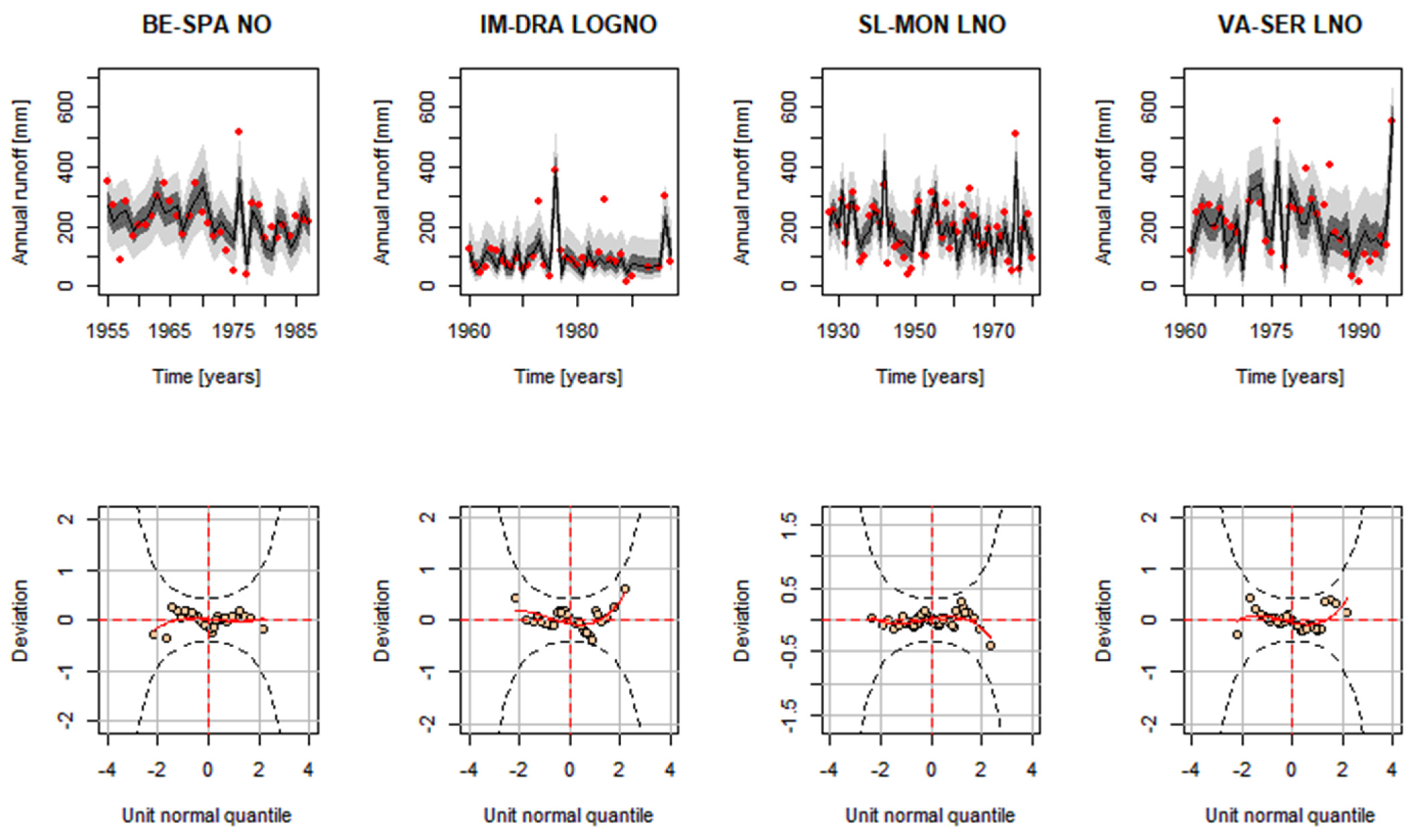
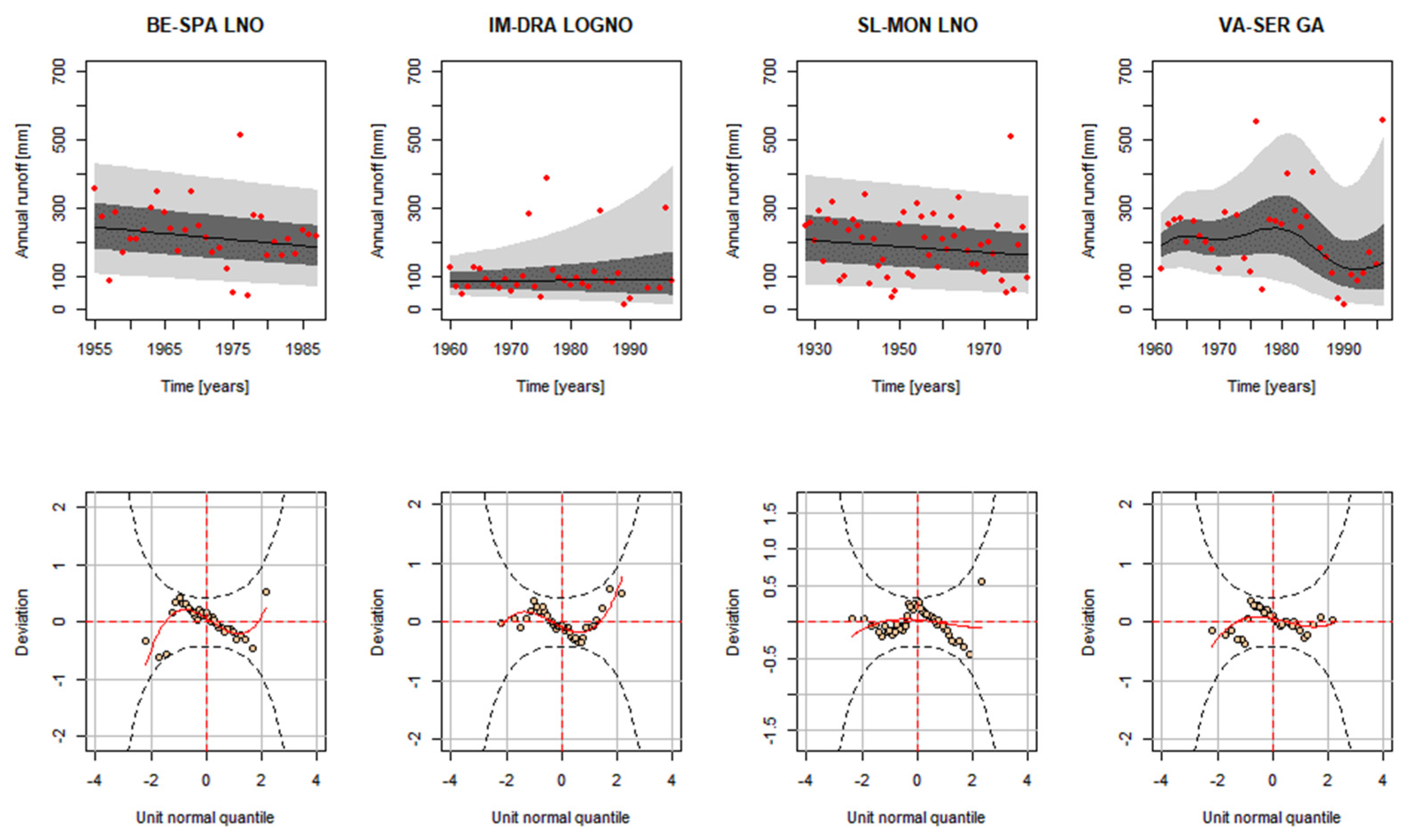
3.3. Non-Stationary Analysis with Time as a Covariate

A further GAMLSS analysis was carried out considering time as a covariate. Again, three non-stationary analyses (see Table 3) were carried out in which (T1) the location parameter μ was modeled as a linear function with respect to time and the scale parameter σ was a constant (µ~t, σ~c), (T2) the location parameter μ and σ were modeled as linear functions of time (µ~t, σ~t) and (T3) the parameter μ was modelled as a cubic spline of time and σ as a linear function of time (µ~cs(t), σ~t). “~c” means that the µ/σ parameter was constant, “~t” means that the µ/σ parameter was modelled as a linear function of time and “~cs(t) means that the µ/σ parameter was modelled as a cubic spline of time.
Figure 9 shows the centile plots and worm plots for the models that provided the lowest AIC values. These are the T1 models for the BE-SPA and SL-MON sites, considering the LNO distribution in the two cases. In contrast, the T2 model was to be preferred for the IM-DRA station, along with the LOGNO distribution. Regarding VA-SER, the T3 model was the best, using the GA distribution.
While the variability of the distributions over time remained almost constant for the BE-SPA and SL-MON sites, for VA-SER, the variability had a remarkable effect. In fact, the lowest AIC value was provided by the T3 model with cubic spline, which is the one that best captured the variability of this dataset. In this case, the trends of the curves in the centile plot are characterized by smooth functions that widen for higher values of the runoff variables. Just as with the IM-DRA values, centiles below 50% show a mainly decreasing trend, while the opposite can be recognized for centiles above 50%. Due to the higher runoff values, especially in the last years of the IM-DRA time series, the variability of the distribution with reference to the 75–95% range increases.
For the IM-DRA and VA-SER stations, the non-stationary analyses with time as covariate provided better AIC values than the stationary analyses.
For the other gauge sites, however, small differences in AIC values were obtained compared to the stationary analysis, which showed slightly better performance. This was unlike the case where rainfall was used as a covariate. In fact, there was no clearly marked trend in the distribution parameters associated with time, and this led to a deterioration in the predictive capabilities of the model compared with the cases which used precipitation as a covariate.
Furthermore, in Figure 9, all points can be seen to be within the 95% confidence band in the worm plots, but the trend lines show cubic/quadratic behavior, except for the SL-MON and VA-SER sites. In any case, these trend lines are more pronounced than those obtained using rainfall as covariate, indicating a worsening of the time-based models.
In Table 4, the AIC values for the three different types of non-stationary models are compared with those for the stationary analysis. As one can see from the AIC values, considering time as covariate did not improve the performance of these models with respect to the S model; the non-stationary models had worse performances, except for the VA-SER site.

4. Conclusions

One of the basic assumptions made in hydrological studies has been that the parameters of the distributions of hydrological variables of interest are constant over time. The use of a stationary probability distribution, therefore, may be ineffective when the examined variable is characterized by change in the mean and/or in variability due to the presence of hydrological change (change in land use or climatic change). In fact, the classical approach to stationary distributions does not take into account the natural variability of certain hydrological processes, such as runoff. It also does not consider changes that may occur in related variables, such as precipitation and temperature, where changes related to climate change may occur.
For these reasons, a GAMLSS model was applied to four Sicilian annual runoff time series to compare classical stationary frequency analysis with different non-stationary frequency analyses, in which, first, annual rainfall and then time were considered as covariates; the distributions investigated were the normal, gamma, two-parameter lognormal, and three-parameter lognormal distributions.
Three different models were developed for the non-stationary analyses. While the first assumed a linear relationship between the location parameter of the distributions and mean annual rainfall, used as covariate, the second exploited a linear relationship between location and shape parameter and the covariate, and the third modeled the relationship between location parameter and the covariate as a cubic spline, maintaining the linear dependence of the shape parameter. The goodness of fit of the models was evaluated by the AIC method, and worm plots were derived to find which distributions best fitted the dependence between rainfall and runoff and between time and runoff. It was also found that, in moving from parametric (i.e., linear) to non-parametric (i.e., cubic-spline) models, on average, the goodness of fit of the distributions provided by AIC remained constant for the different analyzed cases. In general, the best model was characterized by a linear variation of scale and shape parameters as functions of precipitation, while the most frequently preferred distribution, as determined by AIC testing, was the three-parameter lognormal distribution.
While, at present, many studies use temporal variables as covariates in non-stationary hydrological frequency analyses, in this work the introduction of time as a covariate did not improve the performance metrics because of the absence of statistically significant temporal trends in the response variables.
In general, the comparison of different types of models indicates that non-stationary models with observed annual rainfall series as covariates capture the variability of observed data better than stationary models and non-stationary models with time as a covariate. These results confirm that it is necessary but also effective to include physical covariates in the non-stationary frequency analysis of runoff series.
Ultimately, the versatility of these models lies in being able to update the probability distribution of the response variable as a function of time (if a marked trend is present or if there are changes in the source variables, as was the case here). The resulting distributions then allow one to consider an increase/decrease in variability and changes in the mean and variance of the distributions used as a function of future changes in precipitation (or even temperature, for example).
A future development of this study could consist of the derivation of rainfall forecasts from seasonal models or climate models after opportune downscaling, obtaining forecasts of runoff distribution as outputs. Another possibility is to improve the various models by using other covariates, such as temperature, this being one of the main climate variables used to capture climate-change signals. In this perspective, it is possible to expand the dataset of watersheds in order to carry out a regionalization of the non-stationary distribution by introducing basin stationary parameters (e.g., curve numbers, impermeable percentage areas of watersheds, population data, etc.).

Author Contributions

Conceptualization, L.V.N.; methodology, P.S.; software, P.S. and D.T.; validation, L.V.N. and G.C.; formal analysis, P.S.; investigation, P.S., G.C. and L.V.N.; resources, L.V.N.; data curation, P.S., D.T. and G.C.; writing—original draft preparation, P.S., D.T. and G.C.; writing—review and editing, P.S., G.C., D.T. and L.V.N.; visualization, P.S., G.C., D.T. and L.V.N.; supervision, L.V.N.; project administration, L.V.N.; funding acquisition, L.V.N. All authors have read and agreed to the published version of the manuscript.

Funding

This research received no external funding.

Data Availability Statement

Conflicts of Interest

The authors declare no conflict of interest.

References

  1. Cannarozzo, M.; Noto, L.; Viola, F.; la Loggia, G. Annual Runoff Regional Frequency Analysis in Sicily. Phys. Chem. Earth Parts A/B/C 2009, 34, 679–687. [Google Scholar] [CrossRef]
  2. Markovic, R.D. Probability Functions of the Best Fit to Distributions of Annual Precipitation and Runoff Hydrology. Doctoral Dissertation, Colorado State University, Fort Collins, CO, USA, 1965. Paper No. 8. [Google Scholar]
  3. Vogel, R.M.; Wilson, I. Probability distribution of annual maximum, mean, and minimum streamflows in the united states. J. Hydrol. Eng. 1996, 1, 69–76. [Google Scholar] [CrossRef]
  4. Salas, J.D. Analysis and Modeling of Hydrological Time Series. Handb. Hydrol. 1993, 19, 11–72. [Google Scholar]
  5. Liu, L.; Xu, H.; Wang, Y.; Jiang, T. Impacts of 1.5 and 2 °C global warming on water availability and extreme hydrological events in Yiluo and Beijiang River catchments in China. Clim. Change 2017, 145, 145–158. [Google Scholar] [CrossRef]
  6. Donnelly, C.; Andersson, J.C.M.; Arheimer, B. Using flow signatures and catchment similarities to evaluate the E-HYPE multi-basin model across Europe. Hydrol. Sci. J. 2016, 61, 255–273. [Google Scholar] [CrossRef]
  7. Li, S.; Qin, Y. Frequency Analysis of the Nonstationary Annual Runoff Series Using the Mechanism-Based Reconstruction Method. Water 2022, 14, 76. [Google Scholar] [CrossRef]
  8. Sadri, S.; Kam, J.; Sheffield, J. Nonstationarity of low flows and their timing in the eastern United States. Hydrol. Earth Syst. Sci. 2016, 20, 633–649. [Google Scholar] [CrossRef]
  9. Debele, S.E.; Bogdanowicz, E.; Strupczewski, W.G. Around and about an application of the GAMLSS package to non-stationary flood frequency analysis. Acta Geophys. 2017, 65, 885–892. [Google Scholar] [CrossRef]
  10. Jiang, C.; Xiong, L.; Xu, C.Y.; Guo, S. Bivariate frequency analysis of nonstationary low-flow series based on the time-varying copula. Hydrol. Processes 2015, 29, 1521–1534. [Google Scholar] [CrossRef]
  11. Kang, L.; Jiang, S.; Hu, X.; Li, C. Evaluation of return period and risk in bivariate non-stationary flood frequency analysis. Water 2019, 11, 79. [Google Scholar] [CrossRef]
  12. Nasri, B.R.; Bouezmarni, T.; St-Hilaire, A.; Ouarda, T. Non-Stationary Hydrologic Frequency Analysis using B-Spline Quantile Regression. J. Hydrol. 2017, 554, 532–544. [Google Scholar] [CrossRef] [Green Version]
  13. Nogaj, M.; Parey, S.; Dacunha-Castelle, D. Non-stationary extreme models and a climatic application. Nonlinear Processes Geophys. 2007, 14, 305–316. [Google Scholar] [CrossRef]
  14. Villarini, G.; Smith, J.A.; Napolitano, F. Nonstationary modeling of a long record of rainfall and temperature over Rome. Adv. Water Resour. 2010, 33, 1256–1267. [Google Scholar] [CrossRef]
  15. Xiong, L.; Jiang, C.; Du, T. Statistical attribution analysis of the nonstationarity of the annual runoff series of the Weihe River. Water Sci. Technol. 2014, 70, 939–946. [Google Scholar] [CrossRef] [PubMed]
  16. Yang, L.; Smith, J.A.; Wright, D.B.; Baeck, M.L.; Villarini, G.; Tian, F.; Hu, H. Urbanization and climate change: An examination of nonstationarities in urban flooding. J. Hydrometeorol. 2013, 14, 1791–1809. [Google Scholar] [CrossRef]
  17. Koutsoyiannis, D.; Montanari, A. Risks from dismissing stationarity. In Proceedings of the AGU Fall Meeting Abstracts, San Francisco, CA, USA, 15–19 December 2014; p. H54F-01. [Google Scholar]
  18. Matalas, N.C. Comment on the announced death of stationarity. J. Water Resour. Plan. Manag. 2012, 138, 311–312. [Google Scholar] [CrossRef]
  19. Milly, P.C.; Betancourt, J.; Falkenmark, M.; Hirsch, R.M.; Kundzewicz, Z.W.; Lettenmaier, D.P.; Stouffer, R.J. Stationarity is dead: Whither water management? Science 2008, 319, 573–574. [Google Scholar] [CrossRef]
  20. Caracciolo, D.; Noto, L.V.; Istanbulluoglu, E.; Fatichi, S.; Zhou, X. Climate change and Ecotone boundaries: Insights from a cellular automata ecohydrology model in a Mediterranean catchment with topography controlled vegetation patterns. Adv. Water Resour. 2014, 73, 159–175. [Google Scholar] [CrossRef]
  21. Francipane, A.; Fatichi, S.; Ivanov, V.Y.; Noto, L.V. Stochastic assessment of climate impacts on hydrology and geomorphology of semiarid headwater basins using a physically based model. J. Geophys.Res. Earth Surf. 2015, 120, 507–533. [Google Scholar] [CrossRef]
  22. Giuntoli, I.; Renard, B.; Vidal, J.-P.; Bard, A. Low flows in France and their relationship to large-scale climate indices. J. Hydrol. 2013, 482, 105–118. [Google Scholar] [CrossRef]
  23. Giuntoli, I.; Villarini, G.; Prudhomme, C.; Hannah, D.M. Uncertainties in projected runoff over the conterminous United States. Clim. Change 2018, 150, 149–162. [Google Scholar] [CrossRef] [Green Version]
  24. Kormos, P.R.; Luce, C.H.; Wenger, S.J.; Berghuijs, W.R. Trends and sensitivities of low streamflow extremes to discharge timing and magnitude in Pacific Northwest mountain streams. Water Resour. Res. 2016, 52, 4990–5007. [Google Scholar] [CrossRef]
  25. Jiang, C.; Xiong, L.; Yan, L.; Dong, J.; Xu, C.-Y. Multivariate hydrologic design methods under nonstationary conditions and application to engineering practice. Hydrol. Earth Syst. Sci. 2019, 23, 1683–1704. [Google Scholar] [CrossRef]
  26. Li, Y.; Chang, J.; Luo, L.; Wang, Y.; Guo, A.; Ma, F.; Fan, J. Spatiotemporal impacts of land use land cover changes on hydrology from the mechanism perspective using SWAT model with time-varying parameters. Hydrol. Res. 2019, 50, 244–261. [Google Scholar] [CrossRef]
  27. Katz, R.W.; Parlange, M.B.; Naveau, P. Statistics of extremes in hydrology. Adv. Water Resour. 2002, 25, 1287–1304. [Google Scholar] [CrossRef]
  28. Villarini, G.; Smith, J.A.; Serinaldi, F.; Bales, J.; Bates, P.D.; Krajewski, W.F. Flood frequency analysis for nonstationary annual peak records in an urban drainage basin. Adv. Water Resour. 2009, 32, 1255–1266. [Google Scholar] [CrossRef]
  29. Rigby, R.A.; Stasinopoulos, D.M. Generalized additive models for location, scale and shape. J. R. Stat.Soc. Ser. C (Appl.Stat.) 2005, 54, 507–554. [Google Scholar] [CrossRef]
  30. Jiang, C.; Xiong, L.; Wang, D.; Liu, P.; Guo, S.; Xu, C.-Y. Separating the impacts of climate change and human activities on runoff using the Budyko-type equations with time-varying parameters. J. Hydrol. 2015, 522, 326–338. [Google Scholar] [CrossRef]
  31. Li, J.; Tan, S. Nonstationary flood frequency analysis for annual flood peak series, adopting climate indices and check dam index as covariates. Water Resour. Manag. 2015, 29, 5533–5550. [Google Scholar] [CrossRef]
  32. López, J.; Francés, F. Non-stationary flood frequency analysis in continental Spanish rivers, using climate and reservoir indices as external covariates. Hydrol. Earth Syst. Sci. 2013, 17, 3189–3203. [Google Scholar] [CrossRef]
  33. Villarini, G.; Strong, A. Roles of climate and agricultural practices in discharge changes in an agricultural watershed in Iowa. Agric. Ecosyst. Environ. 2014, 188, 204–211. [Google Scholar] [CrossRef]
  34. Li, J.; Gao, Z.; Guo, Y.; Zhang, T.; Ren, P.; Feng, P. Water supply risk analysis of Panjiakou reservoir in Luanhe River basin of China and drought impacts under environmental change. Theor. Appl. Climatol. 2019, 137, 2393–2408. [Google Scholar] [CrossRef]
  35. Stasinopoulos, M.; Rigby, B.; Akantziliotou, C. Instructions on how to use the gamlss package in R Second Edition. 2008. Available online: http://gamlss.com/wp-content/uploads/2013/01/gamlss-manual.pdf (accessed on 1 August 2022).
  36. Akaike, H. A new look at the statistical model identification. IEEE Trans. Autom. Control. 1974, 19, 716–723. [Google Scholar] [CrossRef]
  37. Akaike, H. On the likelihood of a time series model. J. R. Stat.Soc. Ser. D (Stat.) 1978, 27, 217–235. [Google Scholar] [CrossRef]
  38. Nelson, D.B. Stationarity and persistence in the GARCH (1, 1) model. Econom. Theory 1990, 6, 318–334. [Google Scholar] [CrossRef]
  39. Shumway, R.; Stoffer, D. Time Series Analysis and Its Applications with R Examples; Springer: New York, NY, USA, 2011; Volume 9. [Google Scholar]
  40. Chen, H.-L.; Rao, A.R. Testing hydrologic time series for stationarity. J. Hydrol. Eng. 2002, 7, 129–136. [Google Scholar] [CrossRef]
  41. Buuren, S.v.; Fredriks, M. Worm plot: A simple diagnostic device for modelling growth reference curves. Stat. Med. 2001, 20, 1259–1277. [Google Scholar] [CrossRef]
  42. Stasinopoulos, M.D.; Rigby, R.A.; Bastiani, F.D. GAMLSS: A distributional regression approach. Stat. Model. 2018, 18, 248–273. [Google Scholar] [CrossRef]
  43. Rigby, R.A.; Stasinopoulos, D.M. A semi-parametric additive model for variance heterogeneity. Stat. Comput. 1996, 6, 57–65. [Google Scholar] [CrossRef]
  44. Rigby, R.A.; Stasinopoulos, M.D. Mean and Dispersion Additive Models. In Statistical Theory and Computational Aspects of Smoothing; Physica-Verlag HD: Heidelberg, Germany, 1996; pp. 215–230. [Google Scholar]
  45. Zhang, T.; Wang, Y.; Wang, B.; Tan, S.; Feng, P. Nonstationary Flood Frequency Analysis Using Univariate and Bivariate Time-Varying Models Based on GAMLSS. Water 2018, 10, 819. [Google Scholar] [CrossRef] [Green Version]
Figure 1. Flow chart of the employed methodology.
Water 14 02848 g001
Figure 2. Locations of the gauges considered in this study and the related catchments overlaid on the perimeter of Sicily.
Water 14 02848 g002
Figure 3. Scatterplots of annual runoff vs. rainfall (first row) and annual runoff vs. time (second row) for IM-DRA, BE-SPA, SL-MON and VA-SER.
Water 14 02848 g003
Figure 4. Empirical and theoretical cumulative distribution functions (cdfs) and worm plots for the distributions with the lowest AIC values for all the stations.
Water 14 02848 g004
Figure 5. Variation of µ and σ parameters with annual rainfall for the IM-DRA LOGNO distribution (left panel) and the centiles plot (right panel) for the same station, along with the plot for annual runoff vs. annual rainfall.
Water 14 02848 g005
Figure 6. Summary of results for the P1 model for all the stations with generalized additive models in location, scale and shape parameters and the corresponding worm plots for runoff series. The legend for the (first line) is the same as in Figure 5.
Water 14 02848 g006
Figure 7. Best suitable distribution centile curves (first row) and the corresponding worm plots (second row) for the P2 model. The legend for the first line is the same as in Figure 5.
Water 14 02848 g007
Figure 8. Best suitable distribution centile curves (first row) and the corresponding worm plots (second row) for the µ~cs(p), σ~p model. The legend for the first line is the same as in Figure 5.
Water 14 02848 g008
Figure 9. Centiles plots (first row) of the best model for the four considered stations. In the (second row) the corresponding worm plots are displayed. The legend for the first line is the same as in Figure 5.
Water 14 02848 g009
Table 1. Probability density functions with related distribution moments.
DistributionsProbability Density FunctionDistribution Moments
Normal (NO) f ( x ) = 1 σ 2 π e 1 2 ( x μ σ ) 2 E [ x ] =   μ   ;
Var [ x ] =   σ 2   ;
Gamma (GA) f ( x ) = 1 σ μ Γ ( μ ) x μ 1 e x σ E [ x ] =   μ   ;
Var [ x ] =   σ 2   μ 2
Log-normal 2 parameters (LOGNO) f ( x ) = e ( ln ( x )   μ ) 2 2 σ 2   x 2 π   σ E [ x ] = φ 1 2   e μ   ;
Var [ x ] =   φ   ( φ 1 )   e 2   μ ;
where φ = e σ 2
Log-normal 3 parameters (LNO) f ( x ) = 1 2 π ν ( x μ ) e 1 2 ( log ( x μ ) σ ν ) 2 E [ x ] =   μ + e σ + ν 2 2 ;
Var [ x ] = ( e ν 2 1 )   e 2   σ +   ν 2   ;
E 3 [ x ] = ( e ν 2 + 2 ) e ν 2 1 ;
Table 2. AIC values for all the considered distributions of the stationary analysis. In bold are shown the lowest AIC values among the analyzed distributions for each station.
AIC Values
DistributionsBE-SPAIM-DRASL-MONVA-SER
Normal (NO)394.90410.29632.50440.18
Gamma (GA)396.54386.01630.31435.31
Log-normal 2 parameters (LOGNO)402.17380.99635.66441.47
Log-normal 3 parameters (LNO)394.64390.44629.31434.29
Table 3. Comparison of the best stationary and non-stationary models with rainfall as covariate. In bold are shown the distributions that provided the lowest AIC values between the analyzed distributions for each station.
AIC Values
ModelsBE-SPAIM-DRASL-MONVA-SER
S—StationaryLNO
394.64
LOGNO
380.79
LNO
629.31
LNO
434.29
P1—µ~p, σ~cLNO
373.41
LOGNO
365.33
NO
581.02
LNO
409.10
P2—µ~p, σ~pNO
373.36
LOGNO
361.12
LNO
580.46
LNO 407.57
P3—µ~cs(p), σ~pNO
374.66
LOGNO
362.94
LNO
584.36
LOGNO
405.71
Table 4. Comparison of the stationary and non-stationary best models with time as covariate. In bold are shown those models which provided the lowest AIC values among the non-stationary models.
AIC Values
ModelsBE-SPAIM-DRASL-MONVA-SER
S—StationaryLNO
394.64
LOGNO
380.79
LNO
629.31
LNO
434.29
T1—µ~t, σ~cLNO
395.48
LOGNO
382.98
LNO
630.21
LNO
434.96
T2—µ~t, σ~tLNO
397.42
LOGNO
380.87
LNO
630.99
GA
429.06
T3—µ~cs(t), σ~tLNO
400.30
LOGNO
383.96
LNO
631.10
GA
428.69
Publisher’s Note: MDPI stays neutral with regard to jurisdictional claims in published maps and institutional affiliations.

