
Simulation of Heat Flow in a Synthetic Watershed: Lags and Dampening across Multiple Pathways under a Climate-Forcing Scenario


Abstract
:1. Introduction and Objectives
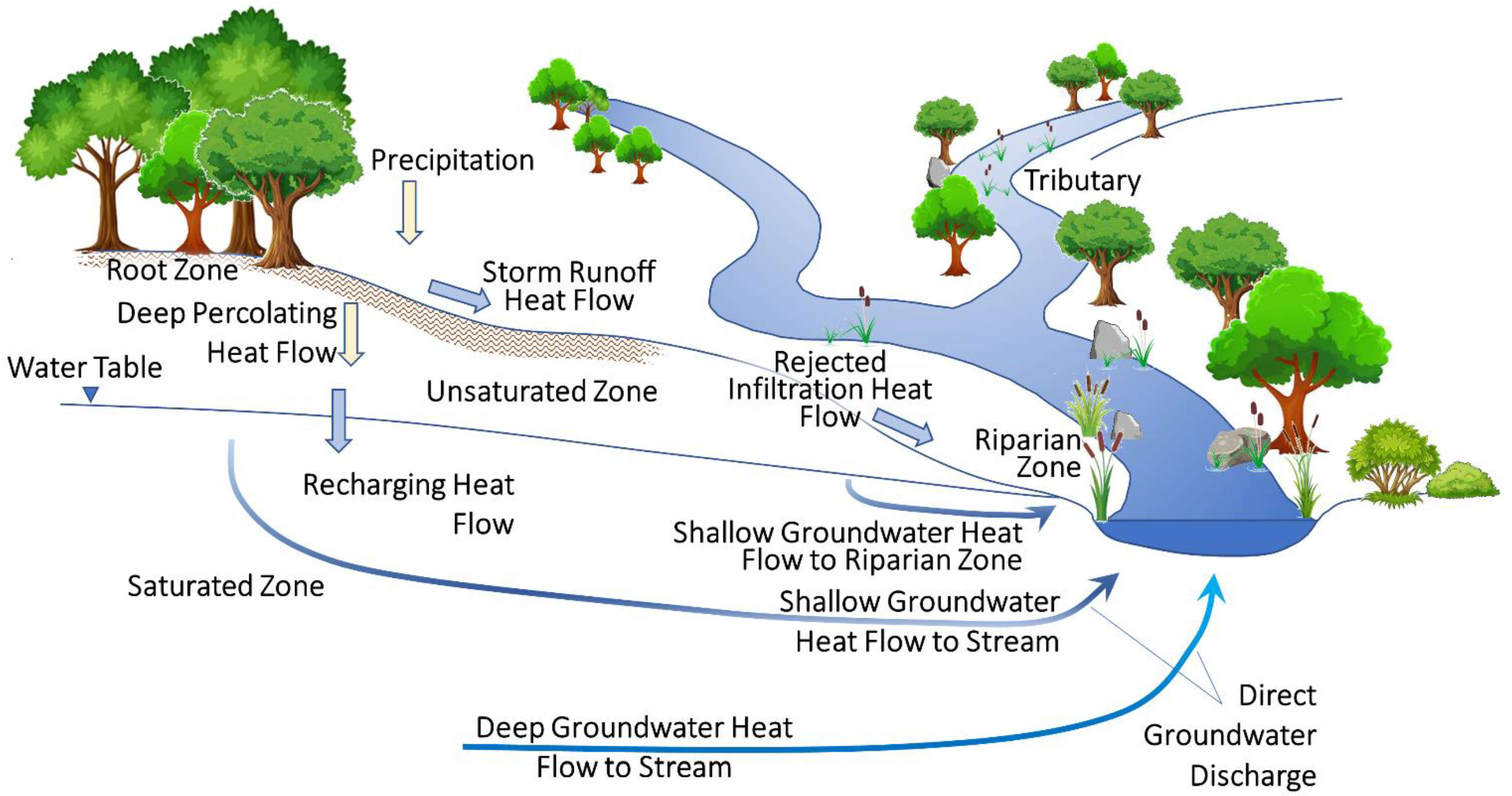
- Heat transport at monthly intervals is explicitly tracked at the watershed scale (1) between the top of the UZ and the water table, (2) between the water table and groundwater discharge zones, and (3) from upstream to downstream in the surface-water network fed by groundwater. The quantification of the heat-flow across various boundaries within a watershed, for example, the water table, enables a more detailed evaluation of the thermal response of a watershed to a changing climate, and in particular to warming infiltration. This type of analysis will be increasingly important as the thermal impacts of a changing climate affect, for example, cold-water fisheries.
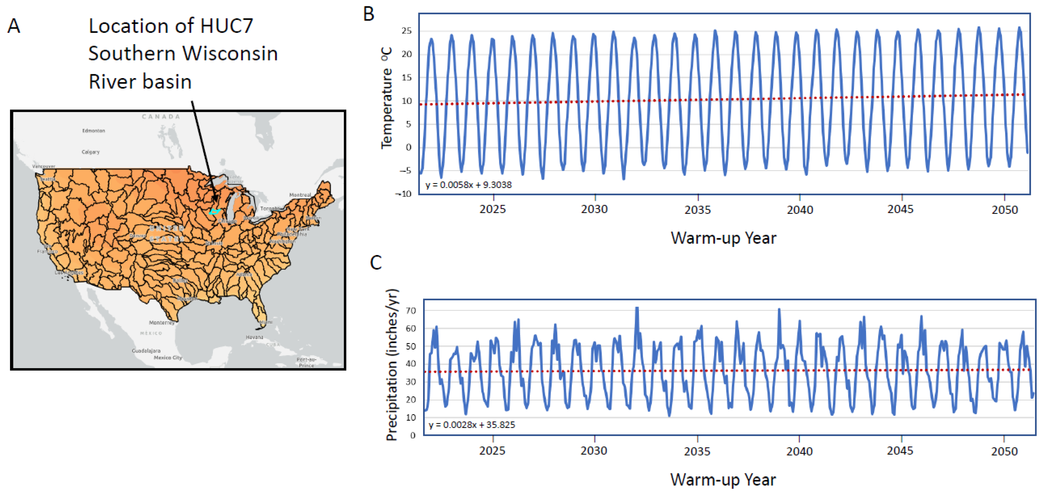
- Whereas Morway et al. [2] employed a heuristic synthetic heat inflow time series to isolate distinct warming effects, this study uses a climate forcing function based on the “mean model” Global Climate Model (GCM) high-emission scenarios [16]. The forcing combines the effects of, first, monthly temperature changes and, second, monthly changes in precipitation that are carried into changes in the infiltration rate through the root zone to the top of the UZ. Application of a specific climate scenario permits a more realistic lag [17] and dampening assessment, which in turn facilitates an extension of these methods to real-world decision support settings.
- In most watersheds, stream flow is a combination of surface (e.g., overland runoff) and subsurface flows. The transfer of heat to the stream network is therefore dependent on both pathways. Variation and extremes observed in stream temperatures tend to be much greater than what is observed in ambient groundwater temperatures-even in baseflow-dominated systems [18,19]. The difference is attributable in large measure to the influence of quick-flowpath additions of storm runoff during warm, wet months that overprint slower/steadier rates of groundwater thermal discharge. Therefore, this analysis expands upon Morway et al. [2] by simulating and analyzing the heat load returned to the surface-water network from storm runoff in addition to the heat load returned by the groundwater system.
2. Methods
- Groundwater runoff is defined as the sum of groundwater discharge to land surface and rejected infiltration from the land surface under conditions of Hortonian or Dunnian flow.
- Baseflow is defined as the sum of direct groundwater discharge to surface water plus groundwater runoff.
- Total streamflow is defined as the sum of baseflow and storm runoff.
- From a watershed flow system perspective, the following partitioning occurs:
- Precipitation is partitioned into infiltration, storm runoff and evapotranspiration (ET) from the root zone.
- Infiltration is partitioned into rejected infiltration, recharge and storage changes in the UZ (no ET is simulated from the UZ since the infiltration is considered to be what percolates below the root zone).
- Recharge is partitioned into storage changes in the groundwater system, direct discharge to surface water and discharge to land surface.
2.1. Construction of Spin-Up and Climate Change Forcing Function
2.2. Model Construction
- spin-up specification of temporally varying infiltration rates and temperatures that, when multiplied, result in a single time-dependent heat infiltration rate that represents a warming climate signal;
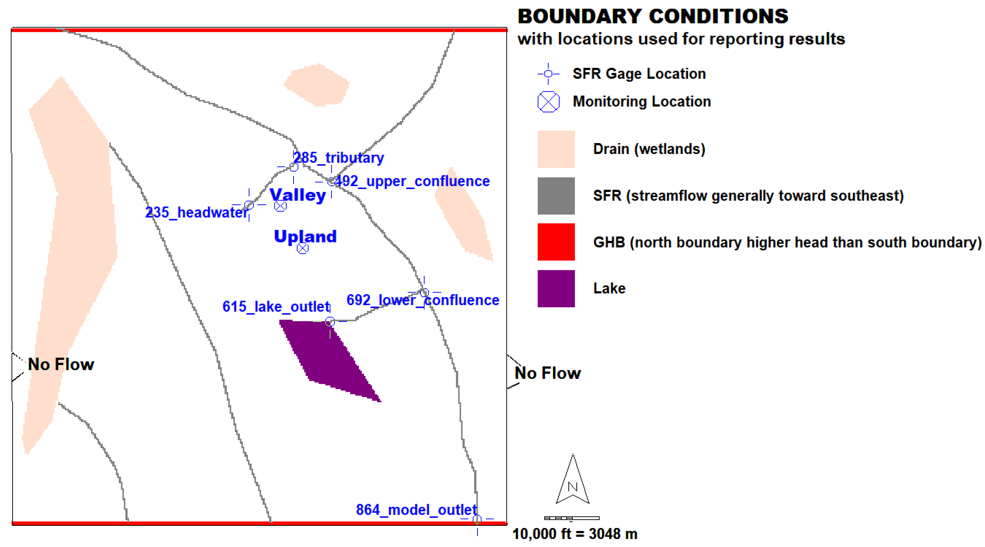
- the climate forcing described in (1) is applied in a spatially uniform manner to the entire model domain; that is, infiltration rates and temperatures are temporally variable but spatially uniform;
- aquifer/flow and transport parameters [e.g., the hydraulic conductivity (flow) and porosity (transport)], are spatially uniform across the model domain.
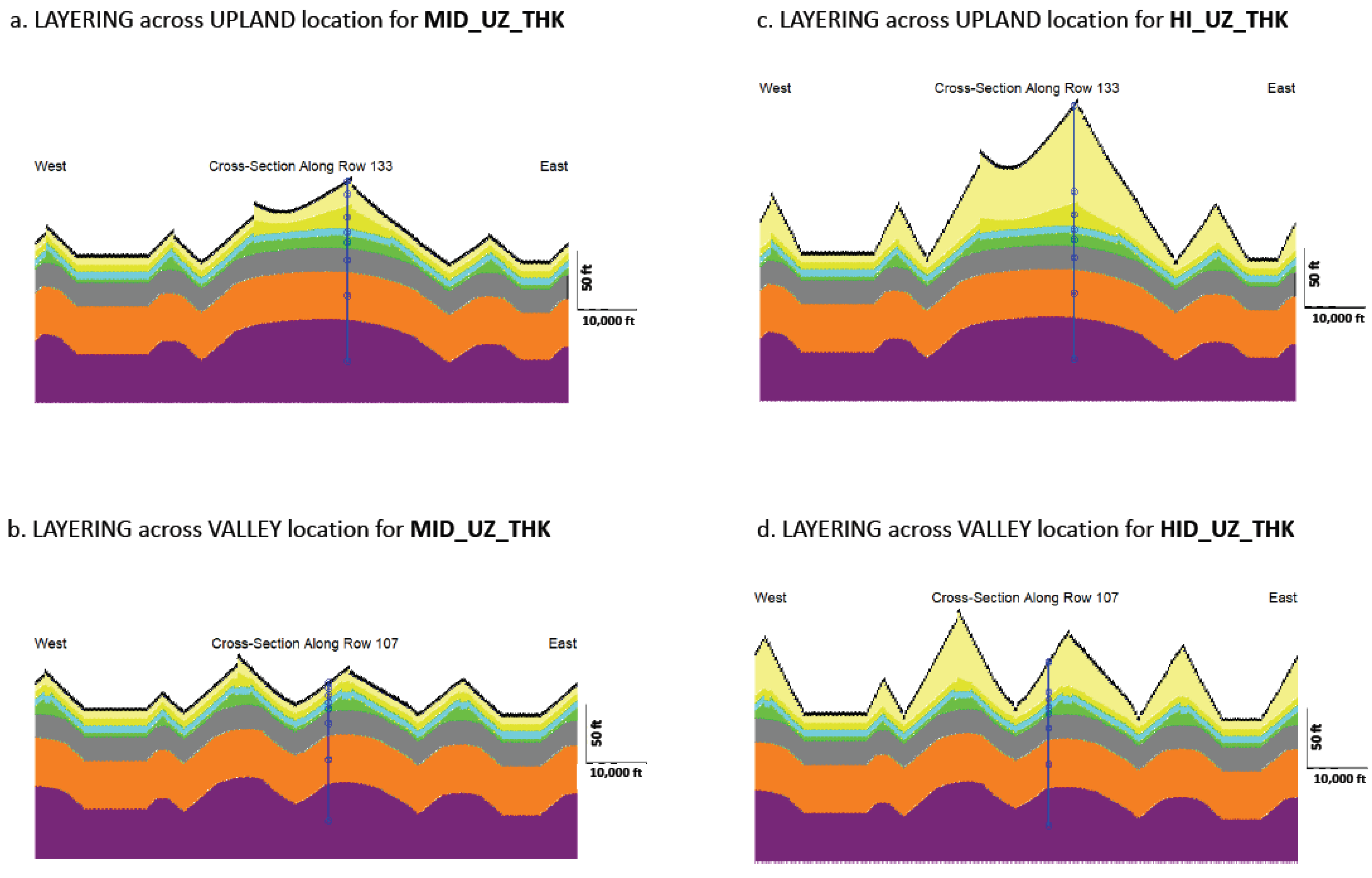
- MID_TRENDED model (Figure 4a,b): This version is designed to produce, on average, a moderate water table depth (i.e., moderate UZ thickness) that varies from 0 m in riparian areas (approximately 20% of the model domain) to about 15 m below land surface in the upland areas.
- HI_TRENDED model (Figure 4c,d): using steeper topography, this version simulates a thicker UZ compared to the MID_TRENDED model. The water table depth varies from 0 m in riparian areas (approximately 4% of the model domain) to more than 30 m in the upland areas.
3. Results and Discussion
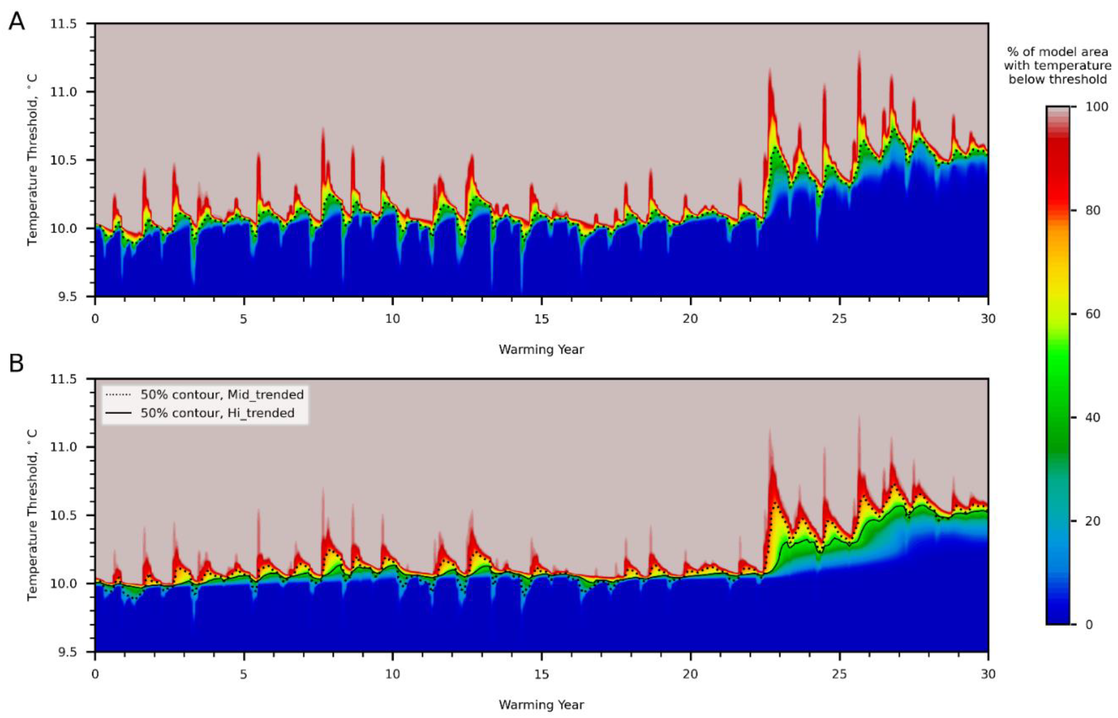
3.1. Temperature Trends along Pathways
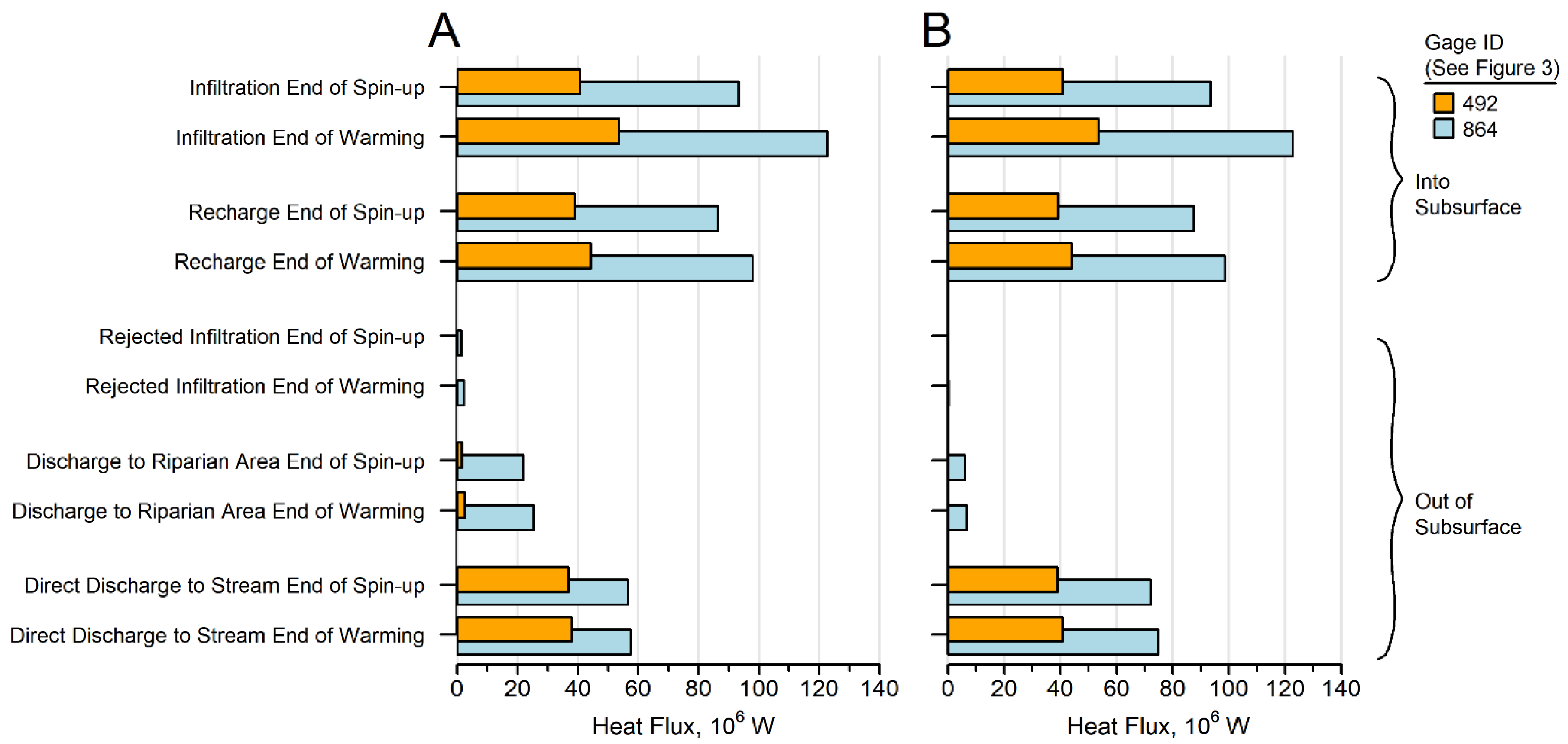
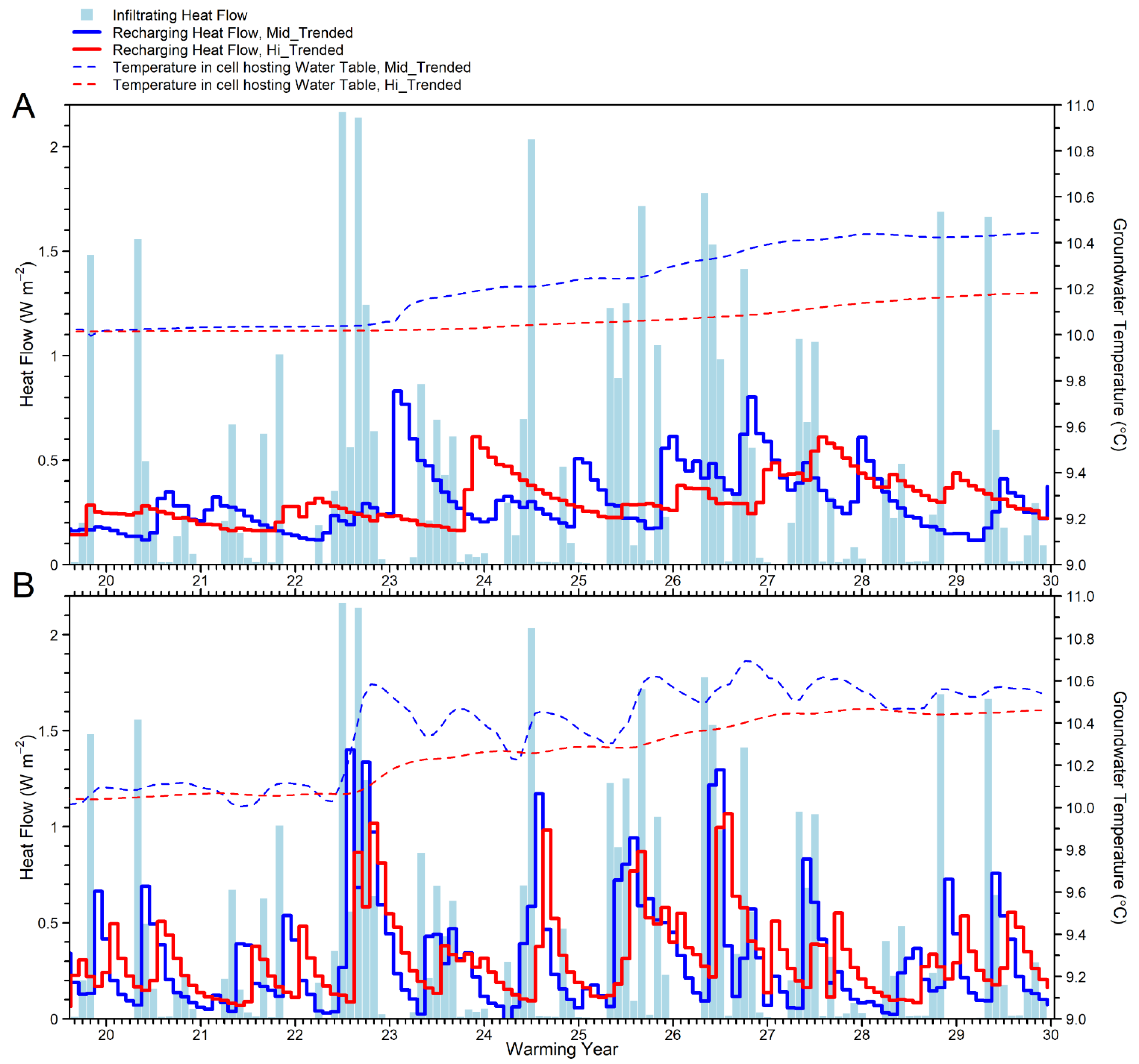
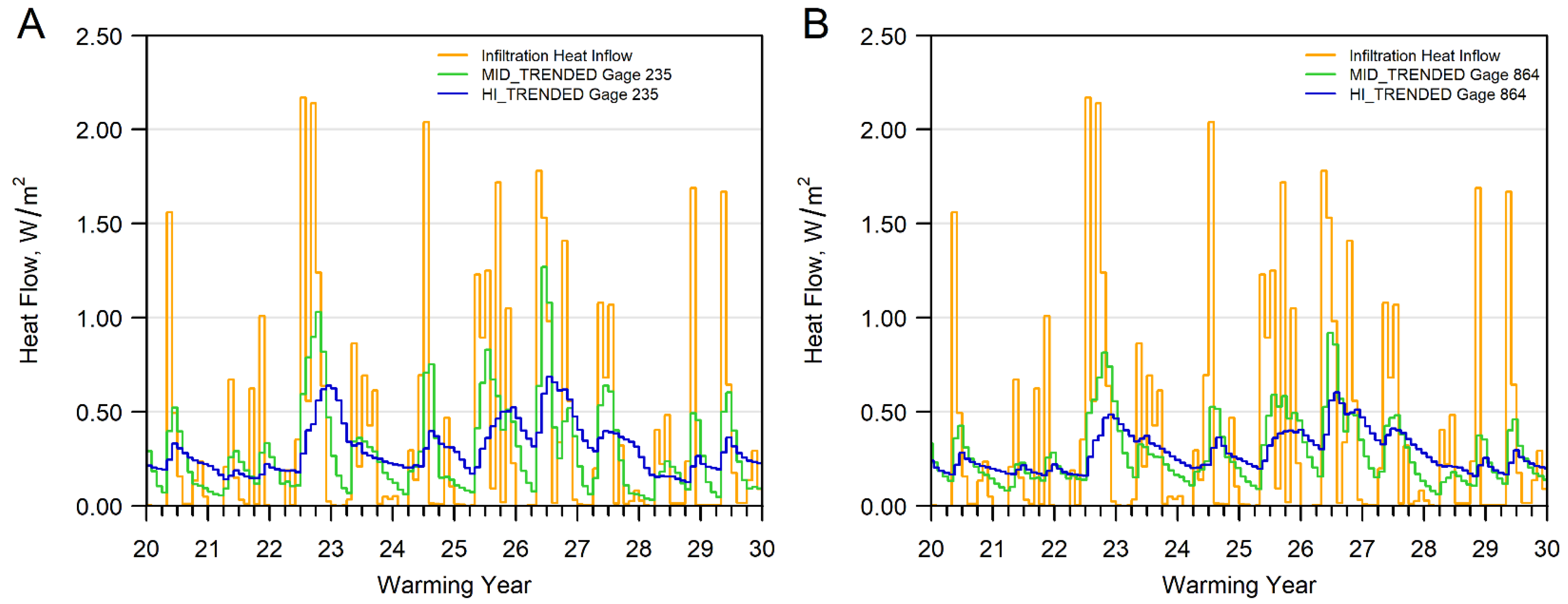
3.2. Heat Fluxes and Heat Flows
- -
- In this study the thermal infiltration is equated with the heat movement downward from the bottom of the root zone which occurs after runoff and evapotranspiration have rerouted some of the water and heat along the land surface or to the atmosphere. This net infiltrating heat flow is imposed as a purely downward convective process into the top of the UZ. For our purposes, the combined effect of heat conduction and dispersion at the root zone/UZ interface, either upward or downward, is considered to be unimportant in comparison to the surface and root zone processes that determine the average monthly rate of infiltrating heat flux.
- -
- Our analysis of the relative weight of simulated heat transport components out of the UZ show that for the humid temperate conditions of the synthetic model, the convective heat flow dominates the conductive and dispersive flow at the water-table interface. This relation persists over time at the scale of individual model locations (Supplementary Material Section S3 Figure S3-10) and when averaged over the entire model domain (Figure 8). For the MID_TRENDED simulation, the absolute value of the conductive heat flows at the water table average about 11% of the convective heat flow, whereas the dispersive heat flow is only 0.05% of the convective heat flow. For the HI_TRENDED simulation, incorporating a generally thicker UZ, the corresponding ratios are 7% and 0.03%. It is worth noting that thermal dispersion is a negligible heat flow component owing to the relatively small longitudinal dispersivity specified (0.9 m) relative to the lateral grid spacing [91 m (300 ft)], a choice consistent with a homogeneous synthetic aquifer. These findings suggest that there is in general only minor loss of accuracy if the heat flow across the interface at the top of the groundwater system is approximated by considering the convective heat flux alone.
- -
- The temperature gradient across the streambed between the stream water in the channel and the ambient groundwater could be incorporated in equations that yield convective and dispersive components of heat flow. Thermal conduction would occur whether the temperature gradient is in the same direction as baseflow or in the opposite direction away from the stream; dispersion would occur only when the gradient is in the same direction as the flow through the streambed. However, the MT3D-USGS code neglects these theoretical components of heat flux and only calculates the convective component, either as a function of groundwater temperature in the presence of baseflow or as a function streamflow temperature in the presence of stream.
3.3. Lags and Dampening of Heat Signal
3.4. Implications for Modeling Watershed Heat Transport
3.5. Limitations and Suggestions for Future Work
- The climate scenarios, appropriately downscaled, are a promising basis for forecasting effects of climate change on watersheds. For the synthetic model, we imposed a linear temperature rise in line with the high-emissions scenario for an area in the Upper Midwest, USA. No effort was made here to partition the expected heat inflow increase among the seasons or months–but this kind of refinement over and above simple linear infiltration trends might be warranted in a real-world application based on different statistical moments of the GCM results for the region under study.
- Similarly, the present study imposed a linear trend on future precipitation and infiltration: expected changes in precipitation intensity and seasonal distribution patterns were neglected but may be important for applications to real-world watersheds.
- A key expansion of the method presented in the companion paper [2] is the inclusion of storm runoff as part of the watershed flow and heat budgets. However, certain thermal mechanisms are still omitted, such as the effect of heat-bearing precipitation and solar radiation on streams as well as the latent heat effects due to evaporation from surface water bodies. Future developments could add these processes to the MT3D-USGS code if sufficiently important for calibration and forecasting.
- This study presents a lagging and dampening analysis of heat flows performed strictly in terms of the convective component. In a real-world application, this approximation, justified for the synthetic model, might not always prove adequate because of the particular importance of conductive and/or dispersive components at watershed interfaces. In such cases, it might be necessary to expand the heat-flow analysis to include all heat transport components, including possibly conduction and dispersion across streambeds. However, it is worth noting that the lagging and dampening analysis in terms of simulated temperature is not an approximation but reflects all heat transport components.
- In this study, the temperature of infiltration at the bottom of the root zone is set equal to the time series of the atmospheric temperature. The assumption may have its validity reduced with time steps shorter than a month or for seasons subject to high rates of evapotranspiration. Additional studies may be needed to determine if and at what time scale temperatures at the top of the UZ can be reliably equated with atmospheric conditions.
- The specific findings presented here regarding lags and dampening correspond to assumed uniform sandy subsurface conditions. In a heterogeneous setting with finer deposits and preferential flow, the phase and amplitude patterns might appreciably change (consider, for example, the effect of confining beds in the unsaturated and/or saturated systems).
- For the synthetic model under study, it was not necessary to impose a calibration period between spin-up and warming periods: only two periods, in this case both set to 30 years, were sufficient for demonstration purposes. However, a real-world application would likely include calibration to historical observations of heads, flows and temperatures. The length of the calibration period would depend on the available data but would need to be long enough to represent properly the transition from the dynamic equilibrium of the pre-calibration spin-up period to the more variable forcing during the calibration and prediction phases.
- If the model setup were modified to extend the warming trends incorporated in the heat inflow forcing function beyond 30 years, the amplitude of the energy and temperature effects over time would of course be magnified. Any applications of the method to real-world settings would likely simulate forecasts into the second half of the 21st century. Given the large degree of uncertainty around future thermal forcing, it is reasonable for applications of the proposed method to real-world watersheds that a range of GCM emission scenarios be considered (as is done in Hunt et al. [18,19]) to treat simulated heat flow findings in a more statistical fashion.
- Monthly time steps may not be sufficiently refined for some forecasts arising from climate warming (for example, fish vulnerability to short-term stream temperature fluctuations). In such cases, simulations with time discretization finer than a month might be warranted, though practitioners may consider restricting temporal refinement of the model to only those stress periods where it is needed.
- The surface-water network in the synthetic model is baseflow-dominated. Losing streams might be more common in a given real-world watershed, but both the MODFLOW and MT3D-USGS codes can handle any combination of gaining and losing conditions with respect to both water and heat flow.
- There are other simplifications adopted in this hypothetical approach that might require more attention in a real-world application. We assumed a no-flow boundary between an unconfined aquifer and underlying bedrock–in real-world settings, the possibility of water and heat loss below an unconfined aquifer might require explicit modeling of deeper units. We equated groundwater contributing area to stretches of stream completely within their topographic basins (Supplementary Material Figure S2-6)–in a real-world study the researcher might want to use the model to delineate groundwater divides more precisely based on the simulated flow system. We also assumed a small dispersivity value of about 0.91 m (3 ft) relative to a grid spacing of 91 m (300 ft). Higher values of dispersivity or identification of preferential pathways could have a strong influence on convection processes. Finally, an important limitation arises from the primitive lake physics in current versions of MODFLOW and MT3D-USGS, where mechanisms such as lake stratification, ice formation, and latent heat transfers during evaporation from surface water are neglected. Such lake processes continue to be subjects of active research that could lead to more sophisticated treatment of water bodies within the watershed thermal regime.
4. Conclusions
- (a)
- to forge a robust approach for applying numerical models to study the hydrologic effects of long-term climate change at the full watershed scale and at a monthly time interval, as deemed appropriate for taking account of how a warming trend imposed on background seasonal and random variability propagates through space from the top of the unsaturated zone downward;
- (b)
- to use a synthetic model of a temperate watershed to not only develop the method but also to draw tentative conclusions about the degree of lagging and damping that a future climate forcing would undergo along distinct surface and subsurface pathways, resulting in predictable changes to the warming signal at unsaturated/saturated and groundwater/surface-water interfaces.
Supplementary Materials
Author Contributions
Funding
Institutional Review Board Statement
Informed Consent Statement
Data Availability Statement
Acknowledgments
Conflicts of Interest
References
- Morway, E.D.; Feinstein, D.T.; Hunt, R.J.; Healy, R.W. New capabilities in MT3D-USGS for Simulating Unsaturated-Zone Heat Transport. Groundwater, 2022; in press. [Google Scholar]
- Morway, E.D.; Feinstein, D.T.; Hunt, R.J. Simulation of heat flow in a synthetic watershed: The role of the unsaturated zone. Water, 2022; in press. [Google Scholar]
- Hunt, R.J.; Prudic, D.E.; Walker, J.F.; Anderson, M.P. Importance of unsaturated zone flow for simulating recharge in a humid climate. Groundwater 2008, 46, 551–560. [Google Scholar] [CrossRef] [PubMed]
- Marçais, J.; Derry, L.A.; Guillaumot, L.; Aquilina, L.; de Dreuzy, J.R. Dynamic contributions of stratified groundwater to streams controls seasonal variations of streamwater transit times. Water Resour. Res. 2022, 58, e2021WR029659. [Google Scholar] [CrossRef]
- Hunt, R.J.; Wilcox, D.A. Ecohydrology—Why hydrologists should care. Groundwater 2003, 41, 289–290. [Google Scholar] [CrossRef] [PubMed]
- Cogswell, C.; Heiss, J.W. Climate and Seasonal Temperature Controls on Biogeochemical Transformations in Unconfined Coastal Aquifers. J. Geophys. Res. Biogeosci. 2021, 126, e2021JG006605. [Google Scholar] [CrossRef]
- Burns, E.R.; Zhu, Y.; Zhan, H.; Manga, M.; Williams, C.F.; Ingebritsen, S.E.; Dunham, J.B. Thermal effect of climate change on groundwater-fed ecosystems. Water Resour. Res. 2017, 53, 3341–3351. [Google Scholar] [CrossRef]
- Suzuki, H.; Nakatsugawa, M.; Ishiyama, N. Climate Change Impacts on Stream Water Temperatures in a Snowy Cold Region According to Geological Conditions. Water 2022, 14, 2166. [Google Scholar] [CrossRef]
- Yao, Y.; Tian, H.; Kalin, L.; Pan, S.; Friedrichs, M.A.; Wang, J.; Li, Y. Contrasting stream water temperature responses to global change in the Mid-Atlantic Region of the United States: A process-based modeling study. J. Hydrol. 2021, 601, 126633. [Google Scholar] [CrossRef]
- Mancewicz, L.K.; Davisson, L.; Wheelock, S.J.; Burns, E.; Poulson, S.R.; Tyler, S.W. Impacts of Climate Change on Groundwater Availability and Spring Flows: Observations from the Highly Productive Medicine Lake Highlands/Fall River Springs Aquifer System. J. Am. Water Resour. Assoc. 2021, 57, 1021–1036. [Google Scholar] [CrossRef]
- Caldwell, T.G.; Wolaver, B.D.; Bongiovanni, T.; Pierre, J.P.; Robertson, S.; Abolt, C.; Scanlon, B.R. Spring discharge and thermal regime of a groundwater dependent ecosystem in an arid karst environment. J. Hydrol. 2020, 587, 124947. [Google Scholar] [CrossRef]
- Hemmerle, H.; Bayer, P. Climate change yields groundwater warming in Bavaria, Germany. Front. Earth Sci. 2020, 8, 523. [Google Scholar] [CrossRef]
- Benz, S.A.; Bayer, P.; Winkler, G.; Blum, P. Recent trends of groundwater temperatures in Austria. Hydrol. Earth Syst. Sci. 2018, 22, 3143–3154. [Google Scholar] [CrossRef]
- Cartwright, J.; Johnson, H.M. Springs as hydrologic refugia in a changing climate? A remote-sensing approach. Ecosphere 2018, 9, e02155. [Google Scholar] [CrossRef]
- Blum, P.; Menberg, K.; Koch, F.; Benz, S.A.; Tissen, C.; Hemmerle, H.; Bayer, P. Is thermal use of groundwater a pollution? J. Contam. Hydrol. 2021, 239, 103791. [Google Scholar] [CrossRef] [PubMed]
- IPCC (Ed.) Climate Change 2022: Impacts, Adaptation, and Vulnerability, Technical Summary; Cambridge University Press: Cambridge, UK, 2022. [Google Scholar]
- Markle, J.M.; Schincariol, R.A. Thermal plume transport from sand and gravel pits–Potential thermal impacts on cool water streams. J. Hydrol. 2007, 338, 174–195. [Google Scholar] [CrossRef]
- Hunt, R.J.; Walker, J.F.; Selbig, W.R.; Westenbroek, S.M.; Regan, R.S. Simulation of Climate-change Effects on Streamflow, Lake Water Budgets, and Stream Temperature using GSFLOW and SNTEMP, Trout Lake Watershed, Wisconsin; U.S. Geological Survey Scientific Investigations Report 2013-5159; U.S. Geological Survey: Reston, VA, USA, 2013; 118p. [CrossRef]
- Hunt, R.J.; Westenbroek, S.M.; Walker, J.F.; Selbig, W.R.; Regan, R.S.; Leaf, A.T.; Saad, D.A. Simulation of Climate Change Effects on Streamflow, Groundwater, and Stream Temperature Using GSFLOW and SNTEMP in the Black Earth Creek Watershed, Wisconsin; 2328-0328; U.S. Geological Survey, Scientific Investigations Report 2016-5091; U.S. Geological Survey: Reston, VA, USA, 2016; pp. 1–117. [CrossRef]
- Niswonger, R.G.; Panday, S.; Ibaraki, M. MODFLOW-NWT, a Newton Formulation for MODFLOW-2005; U.S. Geological Survey: Reston, VA, USA, 2011; p. 44. [CrossRef]
- Bedekar, V.; Morway, E.D.; Langevin, C.D.; Tonkin, M.J. MT3D-USGS Version 1: A U.S. Geological Survey Release of MT3DMS Updated with New and Expanded Transport Capabilities for Use with MODFLOW; 2328-7055; U.S. Geological Survey: Reston, VA, USA, 2016. [CrossRef]
- Gunawardhana, L.N.; Kazama, S.J.J.O.H. Using subsurface temperatures to derive the spatial extent of the land use change effect. J. Hydrol. 2012, 460, 40–51. [Google Scholar] [CrossRef]
- Loinaz, M.C.; Davidsen, H.K.; Butts, M.; Bauer-Gottwein, P. Integrated flow and temperature modeling at the catchment scale. J. Hydrol. 2013, 495, 238–251. [Google Scholar] [CrossRef]
- Loinaz, M.C.; Gross, D.; Unnasch, R.; Butts, M.; Bauer-Gottwein, P. Modeling ecohydrological impacts of land management and water use in the Silver Creek basin, Idaho. J. Geophys. Res. Biogeosci. 2014, 119, 487–507. [Google Scholar] [CrossRef]
- Feinstein, D.T.; Hunt, R.J.; Morway, E.D. Supplementary Material to accompany present article: Simulation of heat flow in a synthetic watershed: Lags and dampening across multiple pathways under a climate-forcing scenario. Water, 2022; in press. [Google Scholar]
- Beven, K. Interflow. In Unsaturated Flow in Hydrologic Modeling; Morel-Seytoux, H.J., Ed.; NATO ASI Series; Springer: Dordrecht, The Netherlands, 1989; Volume 275, pp. 191–219. ISBN 978-94-009-2352-2. [Google Scholar] [CrossRef]
- Anderson, M.P.; Woessner, W.W.; Hunt, R.J. Applied Groundwater Modeling: Simulation of Flow and Advective Transport; 0080916384; Academic Press: London, UK, 2015. [Google Scholar] [CrossRef]
- Niswonger, R.G.; Prudic, D.E.; Regan, R.S. Documentation of the Unsaturated-Zone Flow (UZF1) Package for Modeling Unsaturated Flow between the Land Surface and the Water Table with MODFLOW-2005; U.S. Geological Survey Techniques and Methods Report 6-A19; U.S. Geological Survey: Reston, VA, USA, 2006; 62p. [CrossRef]
- USGS. National Climate Change Viewer. Available online: https://www2.usgs.gov/landresources/lcs/nccv/maca2/maca2_watersheds.html (accessed on 31 January 2022).
- Niswonger, R.G.; Prudic, D.E. Documentation of the Streamflow-Routing (SFR2) Package to Include Unsaturated Flow Beneath Streams-A Modification to SFR1; U.S. Geological Survey Techniques and Methods Report 6-A13; U.S. Geological Survey: Reston, VA, USA, 2005; 51p. [CrossRef]
- Zheng, C.; Hill, M.C.; Hsieh, P.A. MODFLOW-2000, the US Geological Survey Modular Ground-Water Model: User Guide to the LMT6 Package, the Linkage with MT3DMS for Multi-Species Mass Transport Modeling; U.S. Geological Survey Open-File Report 2001-82; U.S. Geological Survey: Reston, VA, USA, 2001. [CrossRef]
- Morway, E.D.; Niswonger, R.G.; Langevin, C.D.; Bailey, R.T.; Healy, R.W. Modeling variably saturated subsurface solute transport with MODFLOW-UZF and MT3DMS. Groundwater 2013, 51, 237–251. [Google Scholar] [CrossRef]
- Morway, E.D.; Feinstein, D.T.; Hunt, R.J. MODFLOW-NWT and MT3D-USGS Models for Evaluating Heat Flows, Lags, and Dampening under High Emission Climate Forcing for Unsaturated/Saturated Transport in a Synthetic Watershed. U.S. Geol. Surv. Model Arch. 2022; in press. [Google Scholar] [CrossRef]


| Stream Gage Number | Gage Description | Upstream Topographic Area | |
|---|---|---|---|
| (equated with Gage Recharge, Baseflow and Runoff Areas) | |||
| mile2 | km2 | ||
| 235 | Headwater | 2.07 | 5.35 |
| 285 | Tributary | 12.06 | 31.23 |
| 492 | Upper Confluence | 58.62 | 151.82 |
| 615 | Lake Outlet | 30.34 | 78.59 |
| 692 | Lower Confluence | 107.22 | 277.69 |
| 864 | Model Outlet | 134.38 | 348.04 |
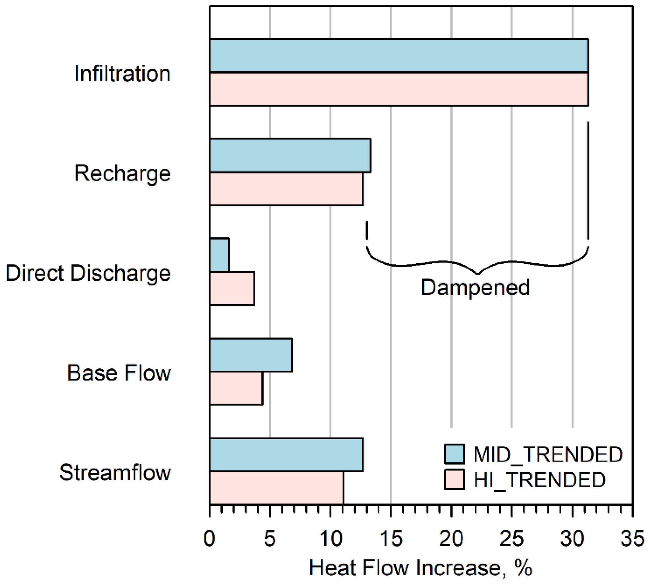
| Heat Flow Pathway | Unit | Location | Model Version | Amplitude Percent Increase Due to Warming 1 |
|---|---|---|---|---|
| Infiltration | Heat flow (Watts/m2) | Uniform across watershed | MID_Trended and HI_Trended | 31.3% |
| Recharge to Water Table | Heat flow (Watts/m2) | Contributing Basin for Model Outlet (864) | MID_Trended HI_Trended | 13.3% 12.7% |
| Direct Discharge to Streams | Heat flow (Watts/m2) | Contributing Basin for Model Outlet (864) | MID_Trended HI_Trended | 1.6% 3.7% |
| Baseflow to Streams | Heat flow (Watts/m2) | Contributing Basin for Model Outlet (864) | MID_Trended HI_Trended | 6.8% 4.4% |
| Total Streamflow | Heat flow (Watts/m2) | Contributing Basin for Model Outlet (864) | MID_Trended HI_Trended | 12.7% 11.1% |
| Heat Flow Pathway | Unit | Location | Model Version | Amplitude Percent Increase Due to Warming 1 |
| Infiltration | Flux-weighted temperature (°C) | Uniform across watershed | MID_Trended and HI_Trended | 22.7% |
| Direct Discharge to Streams | Flux-weighted temperature (°C) | Contributing Basin for Model Outlet (864) | MID_Trended HI_Trended | 1.3% 1.3% |
| Total Streamflow | Flux-weighted temperature (°C) | Contributing Basin for Model Outlet (864) | MID_Trended HI_Trended | 5.6% 5.4% |
Publisher’s Note: MDPI stays neutral with regard to jurisdictional claims in published maps and institutional affiliations. |
© 2022 by the authors. Licensee MDPI, Basel, Switzerland. This article is an open access article distributed under the terms and conditions of the Creative Commons Attribution (CC BY) license (https://creativecommons.org/licenses/by/4.0/).
Share and Cite
Feinstein, D.T.; Hunt, R.J.; Morway, E.D. Simulation of Heat Flow in a Synthetic Watershed: Lags and Dampening across Multiple Pathways under a Climate-Forcing Scenario. Water 2022, 14, 2810. https://doi.org/10.3390/w14182810
Feinstein DT, Hunt RJ, Morway ED. Simulation of Heat Flow in a Synthetic Watershed: Lags and Dampening across Multiple Pathways under a Climate-Forcing Scenario. Water. 2022; 14(18):2810. https://doi.org/10.3390/w14182810
Chicago/Turabian StyleFeinstein, Daniel T., Randall J. Hunt, and Eric D. Morway. 2022. "Simulation of Heat Flow in a Synthetic Watershed: Lags and Dampening across Multiple Pathways under a Climate-Forcing Scenario" Water 14, no. 18: 2810. https://doi.org/10.3390/w14182810
APA StyleFeinstein, D. T., Hunt, R. J., & Morway, E. D. (2022). Simulation of Heat Flow in a Synthetic Watershed: Lags and Dampening across Multiple Pathways under a Climate-Forcing Scenario. Water, 14(18), 2810. https://doi.org/10.3390/w14182810