Article

Designing Efficient and Sustainable Predictions of Water Quality Indexes at the Regional Scale Using Machine Learning Algorithms

by
Abdessamed Derdour
1,*,
Antonio Jodar-Abellan
2,3,
Miguel Ángel Pardo
4,
Sherif S. M. Ghoneim
5,* and
Enas E. Hussein
6
1
Laboratory for the Sustainable Management of Natural Resources in Arid and Semi-Arid Zones, University Center Salhi Ahmed Naama (Ctr Univ Naama), P.O. Box 66, Naama 45000, Algeria
2
Soil and Water Conservation Group, Spanish Research Council, Centro de Edafología y Biología Aplicada del Segura (CEBAS-CSIC), P.O. Box 164, 30100 Murcia, Spain
3
University Institute of Water and Environmental Sciences, University of Alicante, 03690 Alicante, Spain
4
Department of Civil Engineering, University of Alicante, 03690 Alicante, Spain
5
Department of Electrical Engineering, College of Engineering, Taif University, P.O. Box 11099, Taif 21944, Saudi Arabia
6
National Water Research Center, Shubra El-Kheima 13411, Egypt
*
Authors to whom correspondence should be addressed.
Water 2022, 14(18), 2801; https://doi.org/10.3390/w14182801
Submission received: 30 July 2022 / Revised: 23 August 2022 / Accepted: 6 September 2022 / Published: 9 September 2022

Abstract

:
Water quality and scarcity are key topics considered by the Sustainable Development Goals (SDGs), institutions, policymakers and stakeholders to guarantee human safety, but also vital to protect natural ecosystems. However, conventional approaches to deciding the suitability of water for drinking purposes are often costly because multiple characteristics are required, notably in low-income countries. As a result, building right and trustworthy models is mandatory to correctly manage available groundwater resources. In this research, we propose to check multiple classification techniques such as Decision Trees (DT), K-Nearest Neighbors (KNN), Discriminants Analysis (DA), Support Vector Machine (SVM), and Ensemble Trees (ET) to design the best strategy allowing the forecast a Water Quality Index (WQI). To achieve this goal, an extended dataset characterized by water samples collected in a total of twelve municipalities of the Wilaya of Naâma in Algeria was considered. Among them, 151 samples were examined as training samples, and 18 were used to test and confirm the prediction model. Later, data samples were classified based on the WQI into four states: excellent water quality, good water quality, poor water quality, and very poor or unsafe water. The main results revealed that the SVM classifier obtained the highest forecast accuracy, with 95.4% of prediction accuracy when the data are standardized and 88.9% for the accuracy of the test samples. The results confirmed that the use of machine learning models are powerful tools for forecasting drinking water as larger scales to promote the design of efficient and sustainable water quality control and support decision-plans.

1. Introduction

High-quality water resources are vital in the supply of necessary drinking water for humans and natural ecosystems, but also to guarantee human activities and development [1,2]. Nowadays, it is well-studied that several factors interacting in complex systems among them such as population growth, intensive agriculture, urbanization, and industrial activity, increase the water need, especially facing an uncertain context of climate change [3]. According to a recent United Nations (UN) report, 1.5 million people die each year because of diseases caused by contaminated water because water contamination causes 80% of health problems in low-income countries [4]. In fact, five million fatalities and 2.5 billion illnesses were accounted for during the time of this report. Therefore, the assessment and prediction of water quality are required to set up whether water is suitable for a certain use and, if not, to find relevant remedies or precautions; however, water quality is determined by many measures that quantify dissolved substances. Due to this, assessing all interacting factors in a groundwater bodies (and/or in a water surface lagoon) is insufficient in low-income countries because the process is expensive and exhausting [5]. As a result, minimizing the subjectivity and the cost-effectiveness of water quality assessment is a major challenge and several tools are being developed to determine its cleanliness and purity [6,7].
The design of an accurate and adapted Water Quality Index (WQI) is a well-accepted indicator used by several international and national organizations to classify water quality at a certain location and time. Some researchers proposed modifications when calculating this indicator (WQI), for instance, Uddin, Nash [8] presented twenty-one WQI models for assessing drinking water quality, such as the Horton index, the National Sanitation Foundation (NSF-WQI), and the Bascaron index (BWQI), among others. In order to calculate it, physicochemical parameters must be gathered. As a result, an indicator is achieved that allows the general public to know the water quality in aquifers [9]. It can also evaluate water characteristics about human health and natural quality effects [10] or even to decipher its impact on water poverty risk [11].
Indicators such as the WQI often are calculated in a complex and time-consuming process. So, many methodologies are proposed to easily and accurately predict these indicators considering its application for larger scales instead of a specific municipality or small catchment. These models make it possible to expect compliance (and noncompliance) with quality requirements in the short and long terms [12]. Water quality monitoring and forecasting are carried out using a variety of methods such as computational intelligence techniques (such as genetic algorithms, artificial neural networks, and others), which have received increasing attention in environmental time-series prediction research, as they allow for modeling nonlinear systems and are robust to noise data, leading to more right results [13,14,15]. Thus, the machine learning helps to reduce the consumption time to compute the WQI for each sample. However, using equations to determine the WQI for 100 samples will consume more time, while using the machine learning (classification learner) will significantly save the consumed time [12,13,14,15].
Recently, traditional Machine Learning models such as the Decision Tree, which has been frequently used in many fields and applications [16,17] has been applied for water quality assessments. The Ensemble Trees (ET), which is considered a more accurate predictor than any of the individual learning algorithms has been tested [18,19]. Discriminant analysis (DA) was also utilized in several kinds of research around the world to predict water quality by generating discriminant functions (DFs) for grouping nonoverlapping data based on scores on one or more quantitative predictor variables [20,21]. Other researchers even used K-nearest neighbors (KNNs) to classify and predict the water quality [22,23].
Likewise, several new studies have been published assessing the behavior of the WQI by using machine learning algorithms in many regions over the world [24,25]. For instance, Support Vector Machines (SVM) can be offered as a robust technique for water quality prediction in a free-form wetland environment because of many variables influencing water quality [26]. Some approaches adopted SVM to predict sediment load concentration in an arid watershed as in India Samantaray, Sahoo [27], or to predict the boundaries of water quality limits, for example, in the Kelantan River in Indonesia by Kurniawan, Hayder [28]. Koranga, Pant [29] proposed a machine learning model to predict the water quality of Nainital Lake in India. Tan, Yan [30] used a square support vector machine to predict water quality time series data from China. Mohammadpour, Shaharuddin [13] forecasted the WQI in freely constructed wetlands using a support vector machine in Malaysia. Other studies have also been undertaken in Algeria to test the effectiveness of SVM [31,32,33,34] and confirmed that SVM provides accurate results in less time-consuming and can run with fewer data than other algorithms. However, there is a lack of studies that offer decision-makers effective tools for predicting water quality index to improve water resource planning and to be used at larger scales in arid areas.
Therefore, in this research, classification techniques were used to predict the WQI for several water samples collected from an arid area, in particular, the Naama province in Algeria which depicts clear signals of water pollution and scarcity. To accomplish this objective, the MATLAB tool was considered because it contains a set of classification learner methods, such as the SVM among others [35]. The main goals of this study can be summarized as follows: (i) assess the physicochemical properties of different water points (samples) on a large scale (12 municipalities); (ii) determine the water quality of the study area, depending on the WQI; (iii) apply the learner technique to develop a classification model for dry areas estimating the model’s accuracy about WQI values. These data were divided into classes such as excellent, good, poor, and very poor or unsafe water in order to facilitate its consideration; (iv) predict the WQI by using the best classifier, which develops the based prediction accuracy, and (v) offer decision-makers with effective tools for predicting water quality index to improve water resource planning and management in arid areas. We hypothesize that the proposed prediction model will reduce the time to determine the water quality state based on conventional equations.

2. Materials and Methods

2.1. Description of the Study Area and Data Collection

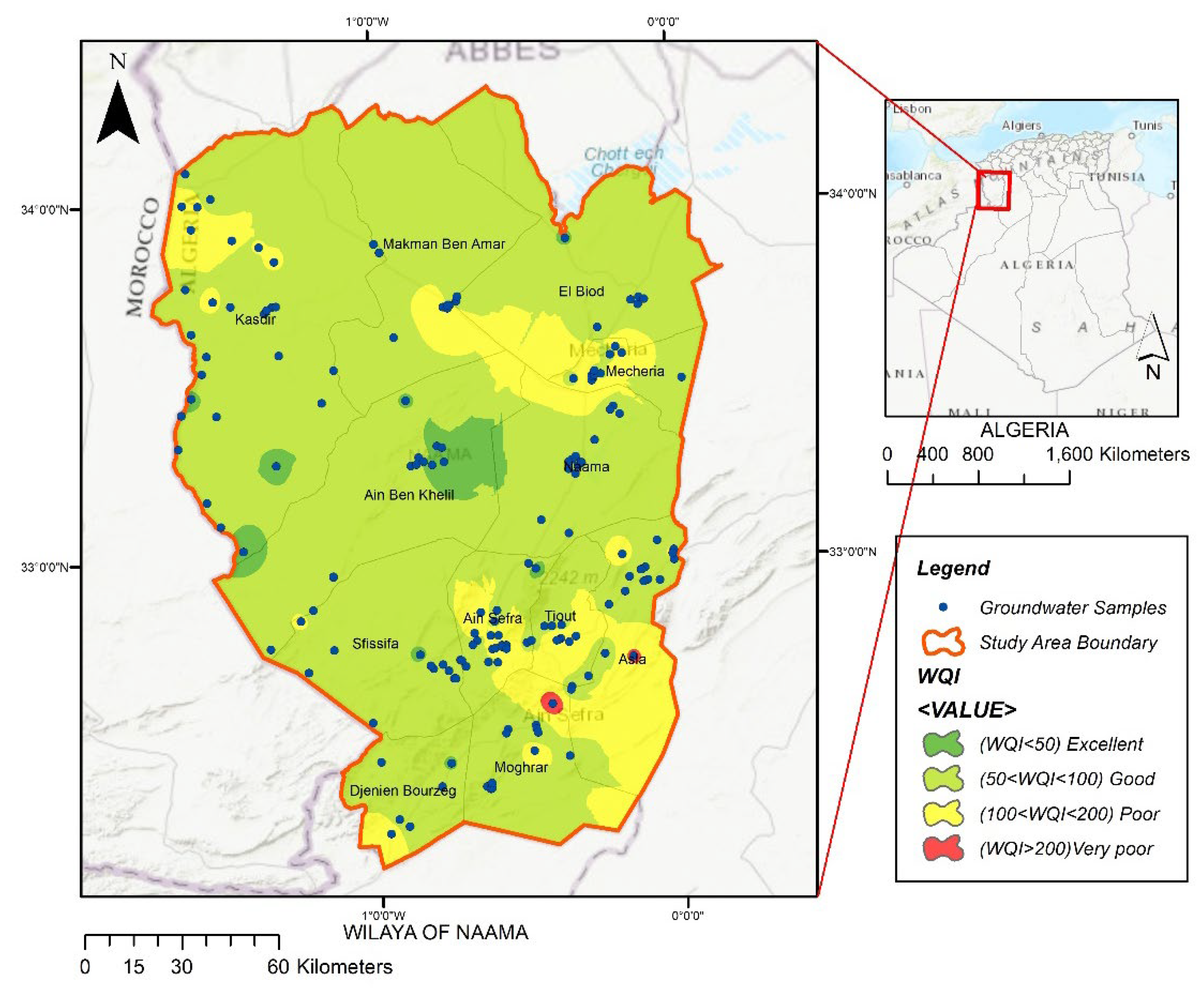
This research was carried out in the region of Naâma (Figure 1), which is located in the southwestern part of Algeria (from 32°9.284′ N to 34°19.492′ N; and from 1°39.568′ W to 0°1.781′ E). It is part of the high plains of southern Oran, a region affected by desertification processes [36], and specifically, the case study area is situated between the Tell Atlas and the Saharan Atlas in the western part of Algeria.
The north region of the Naâma is characterized by pastoral activities, particularly in hilly areas. In contrast, in the south region, agricultural fields with olive orchards, cereals, vegetables, and livestock can be found [37]. Naâma receives most of its rainfall from the north direction, with an estimated average of 287 mm [38]. The evaporation can reach 2000 mm, which affects the groundwater quality. The average temperatures range from 7.22 to 30.03 degrees Celsius. Summer temperatures can reach 48 °C, while in winter, they can drop below 0 °C [39].
The case study area depicts about 29,825 Km2 (i.e., three times the area of Lebanon). Rangelands occupy about 74% of the total area (22,070.50 Km2) and the southern pre-Saharan zone extends over the remaining 14% (4175.50 Km2) [40]. Elevation ranges from 768 to 2239 m.a.s.l. Geologically, Naâma is composed from the Triassic to the Quaternary formations [41]. The vegetation is characterized by a steppe except in the mountains, where remains of Aleppo pine forests (Pinus halepensis Mill.) are identified [42].
The main water resources refer to groundwater used for irrigation and drinking in the region. From a hydrogeological perspective, the Wilaya of Naâma has four main groundwater aquifer systems: the Jurassic sandstone aquifer, the lower cretaceous sandstones aquifer, the tertiary limestones aquifer, and the quaternary alluvial aquifer [43]. Those aquifers offer water supplies to 208,136 people living and there are supplies to 1,792,076 animals grazing in this area. These resources irrigate 43,688 ha of agricultural area. Because of the population growth and several activities developed throughout the study area, it is necessary to assess the water demand and the supply of resources. The dataset in this research was gathered from twelve different communes in the Naâma Province.

2.2. Data Collection, Analysis, Sampling, Preprocessing and Water Quality Index Calculation

A total number of 169 samples were collected to analyze eleven elements. Electric Conductivity (EC), Mineralization, and Hydrogen Power (pH) were measured in situ using a portable HANNA type multiparameter (HI98194) during the sampling procedure in the laboratory at the University Center of Naâma. Then, in the Algerian Water Unit of Naâma (ADE) laboratory, a flame photometer was used to measure Sodium (Na) and Potassium (K). The UV-Vis spectrophotometer recognized Sulphate (SO4) and Nitrate (NO3), and the complex metric titration method was used to identify Calcium (Ca), Magnesium (Mg), Chloride (Cl), Bicarbonate (HCO3). These values were then used to rank the water samples according to many terms that affect water quality [44,45].
This study considers the collected dataset to test the proposed model, and eleven significant water quality parameters are included. WQI has been calculated using the following Formula (1):
W Q I = i = 1 N q i   w i   i N w i
where W Q I , is the water quality index; N represents the total number of parameters used to calculate the WQI.   q i means the rating scale of each parameter, which is determined using Equation (2), where Si denotes the drinking water standards, and Ci denotes the concentration of each chemical parameter (Table 1). Detail information of these equations can be found in [8,9].
q i = C i / S i × 100
Table 1 depicts the relative weight of each physicochemical parameter. In particular, weights were attributed to each of the study’s 11 physicochemical parameters, according to their relative significance on the total quality of drinking water. Thus, nitrates received a maximum weight of 5, due to their high impact on groundwater quality, while magnesium was assigned the minimum value of 1, due to its low influence on the water quality of drinking. Weights between 2 and 4 were attributed to other physicochemical parameters.
The values of WQI were classified into four classes as below [46]: Class I: excellent water class and WQI < 50; Class II: good water class and 50 < WQI < 100; Class III: poor water class and 100 < WQI < 200; and, Class IV: very poor water class and WQI > 200.

2.3. Data Classification

The results obtained from the data samples were divided into training and testing ones (151 and 18 samples, respectively). The limitation of the samples number imposed on us to reduce the number of test samples. A total number of 151 samples were used for training to be efficient and to get a robust classifier model. Although the number of test data is small, it contains all classes. On the other hand, the accuracy of the model will be calculated based on the correct number of predicted samples to the total number of test samples. Thus, the number of samples for each class of the sample data is selected to be sufficient for determining the prediction accuracy. The number of test samples for each WQI class is shown in Table 2.

2.4. Data Standardization

In this study, the original classifiers were applied to the raw data without normalization, and the forecast model was built up. The data standardization was accomplished to study the transformation process of the data on the prediction accuracy of the classification process. It is not easy to compare data from different sources, such as analyses and tests. Therefore, data standardization is an important task to analyze, process, and compare more accurately and efficiently. Each variable value as X is subtracted from the sample’s mean (μ) and divided by the standard deviation (σ). The mean and standard deviation of each data sample of each variable will be zero and 1, respectively. The new standard magnitude of each variable in each sample can be determined as in Equation (3):
X n = X c μ σ
where μ and σ are the mean and standard deviation of each variable for all samples in the training process, respectively.

2.5. Classification Techniques

2.5.1. Decision Tree

The decision tree (DT) is a prediction tool or a classification tool, which uses machine learning [33,45]. The decision tree is a binary tree that means for every parent, there are at most two offspring. Each node in the tree refers to a variable and also a separation point for that variable. Each leaf of the tree represents the result (output) that was used to predict. To build the prediction DT model, the following procedures must be followed: (i) the variables from the data that will build the model should be selected, (ii) choose the values by which separate each variable based on the rules that have been built; and, (iii) tree construction ends upon arrival with a certain stop condition (for example, the lowest number of instances of tree leaves were identified).

2.5.2. Ensemble Tree

A combination of several DTs to get the highest predictive performance than only one DT is referred to ensemble method. It is based on combining the weak learners to compose a strong learner. There are two techniques used in ensemble decision trees, the first one is bagging and the other is boosting [47,48]. The bagging (Bootstrap Assembly) is used when it is necessary to reduce the variance in the DT. The bagging technique basis consists on create several datasets from the randomly selected and replaced training sample. Then, each subset of data is used to train the decision trees. The mean of all predictions is used for various trees and is stronger than a single decision tree. The other ensemble technique is boosting used to create an aggregation of predictors. The learners act consecutively: the first learners adapt simple models to the data, and then the errors are analyzed. It means that consecutive trees (random samples) were adjusted to resolve the net error of the previous tree.

2.5.3. K Nearest Neighbors (KNN)

It is a supervised machine learning classification algorithm and the simplest and most frequently used classifier. In KNN, a new data point is categorized based on similarity in a particular group of neighboring data points. For a given data point in the set, the KNN identifies the distances between this point and all other K points in the dataset close to the initial point and then, votes for the class which is the most common. Usually, the Euclidian distance is taken as a distance measurement. Thus, the resulting final model is just the labeled data placed into space. KNN is used in different applications such as genetics, forecasting, etc. [49].

2.5.4. Discrimination Analysis (DA) Classifier

Discrimination analysis (DA) proposes that various classes produce data based on various Gaussian distributions. For training a DA classifier, the fitting function assesses the parameters of a Gaussian distribution for each class. For predicting the classes of new data, the trained classifier finds the class with the lowest cost of misclassification [50].

2.5.5. Support Vector Machine (SVM)

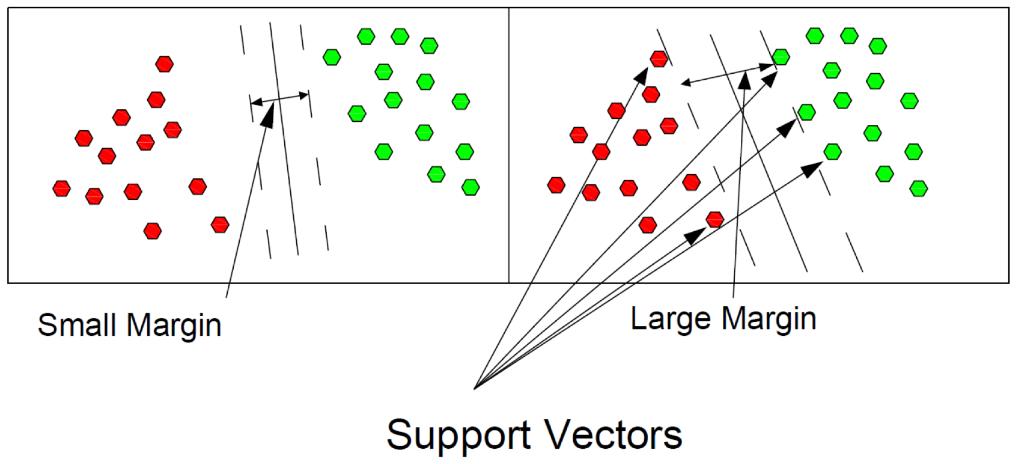
The SVM classification technique gave the highest classification and prediction accuracy of the WQI in the current study. It is a machine learning tool that separates the data into two-class data via a hyperplane [51]. This hyperplane must achieve the greatest distance between the points of each class; then, accurate classifying can occur. If any point lies outside the hyperplane margin, it belongs to a different class. Greater features lead it more difficult to separate among different classes. Figure 2 illustrates the margin condition of SVM. A good classification can occur when a large margin exists [52,53].
Hyperplanes can separate all samples in each WQI class in SVM in multidimensional space. The hyperplanes distinguish between every two WQI classes (Yi and Yj) of WQI of two different input vectors (Xi and Xj) [54]. The hyperplane with the greatest margin must be found among these hyperplanes. An orthogonal vector ω to the hyperplane can be defined as in Equation (4):
ω = ω 1 , ω 2 , , ω k
The hyperplane function, h, can be identified as mentioned in Equation (5) [54]:
h X i = w T .   X i + ω 0 = ω 0 + i = 1 k ω i . x i
where ω 0 is the bias term to determine the separating hyperplane position (i.e., h (X) = 0). One by one learning strategy is chosen, where Xi is the class 1 when h (Xi) ≥ 0 and is −1 elsewhere. If Xi and Xj are the two closest points on each side of the hyperplane (i.e., different classes), the hyperplanes h (Xi) and h (Xj) are:
h X i = w T ·   X i + ω 0 = 1
h X j = w T ·   X j + ω 0 = 1
Differencing these equations and dividing both sides by the magnitude of the ω, we obtain:
X i - X j = 2 ω
where XiXj is the distance between the two hyperplanes.
The maximization of the margin of Equation (8) implies the minimization of the weight vector ω defining the hyperplane. In addition, a soft-margin SVM is utilized for nonlinear classes to allow the model to misclassify some data points by minimizing the number of such samples [55].

3. Results

3.1. Description of the Physicochemical Analysis of the Sampling Points

The results of eleven (11) physicochemical parameters obtained from 169 samples of groundwater in the Wilaya of Naâma are shown in Table 3.

3.2. Water Quality Index Assessment

The results obtained to evaluate the groundwater quality through the Wilaya of Naâma using the WQI method are presented in Table 4, and in Figure 3.

3.3. Results with Raw Data

The procedures to predict the WQI via the classifiers will be illustrated. The data (169 samples) is classified based on the WQI in Excellent, good, poor, and very poor classes (Table 2). A total number of 151 samples were used for training and the remain (18 samples) were used for testing the model. The training and testing samples were selected to include all classes. The 151 samples were trained with all classifiers to investigate which one is the best (achieves high prediction accuracy). This process was accomplished by feeding the classification learner tool in MATLAB with the input data of each sample and its output (WQI). So, the classifiers learn the relation between the inputs and outputs (extraction the features). Each class will contain the samples that have similar features. After learning the classifier, the constructed weighted matrix (identifying the features of each class) was exported to the worksheet in MATLAB and then the test data were applied without its output and then the prediction results will be developed based on the feature in weighted matrix for each class. Then the accuracy of the constructed classifier will be computed dividing the number of the correct prediction to the total number of test data (18 Samples).
The samples’ raw data was first considered by comparing its results with the standardization data. When all classification techniques are applied to the raw data, Linear SVM presents the highest accuracy of the classification process in the training stage (94.7%), as shown in Table 5. The results of training the classifiers on the raw data illustrate that the SVM classifier developed the highest accuracy rather than the other classifiers. It develops notable correctness with less computation power and is preferable in classification problems. It is also used when an understandable margin of dissociation between classes is observed. Likewise, it is suitable for high dimension spaces and considers memory systematic.
Other techniques obtained similar results, 93.4% for the quadratic SVM, and the cubic SVM and linear discrimination classifiers provide lower values, such as 90.7 and 88.7%.
The cross-validation method is used in classifier learners to investigate the constructed prediction model’s robustness and to verify the model’s prediction accuracy. In this method, the data samples divide into two partitions for the training and testing processes. Division of the data samples was carried out randomly into k equal size subsamples. A single subsample is kept as validation data. The remaining k-1 subsamples are used in training the model and repeated k times. The accuracy of the test data is average to develop the final model accuracy. So, all data samples are used for training and validation processes [57]. The stratified k-fold cross-validation is used in the classification learner to solve the classification problem so that the folds are selected. Each selected fold randomly includes the same features as each categorized class.
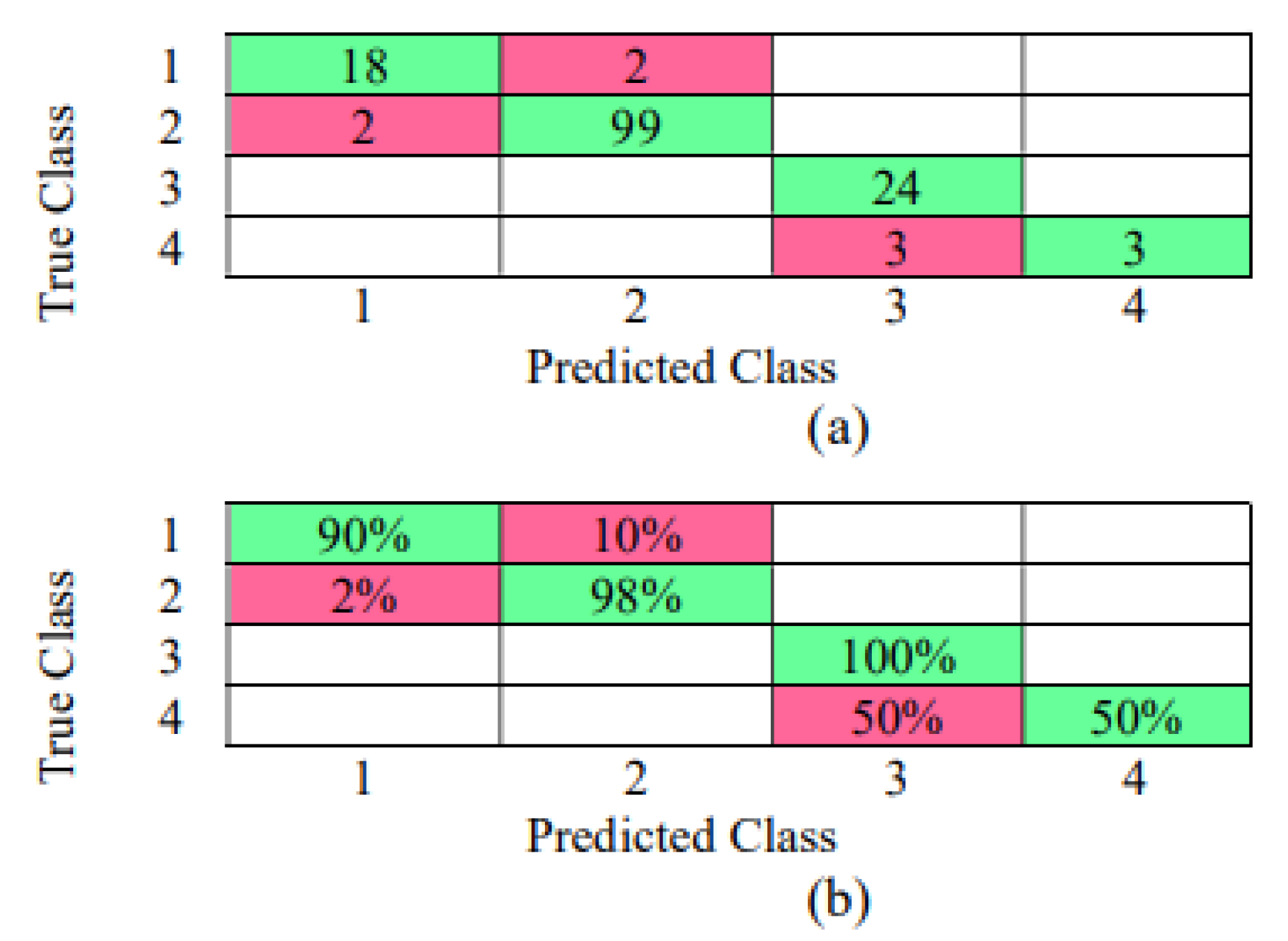
Figure 4 shows the linear SVM confusion matrix achieved with the classification technique. Figure 4a shows the corrected prediction samples for each class. The “excellent” WQI (class 1) was correctly classified in 17 out of 20 samples; in class 2, 99 out of 101 samples were correctly predicted. Figure 4b explained the prediction accuracy of each class, where the correct prediction of class 1 (Excellent state) was 85% (17/20), and the wrong prediction was 15% (3/20). For the very poor state, the correct and wrong predictions were 50% (3/6) and 50% (3/6), respectively.
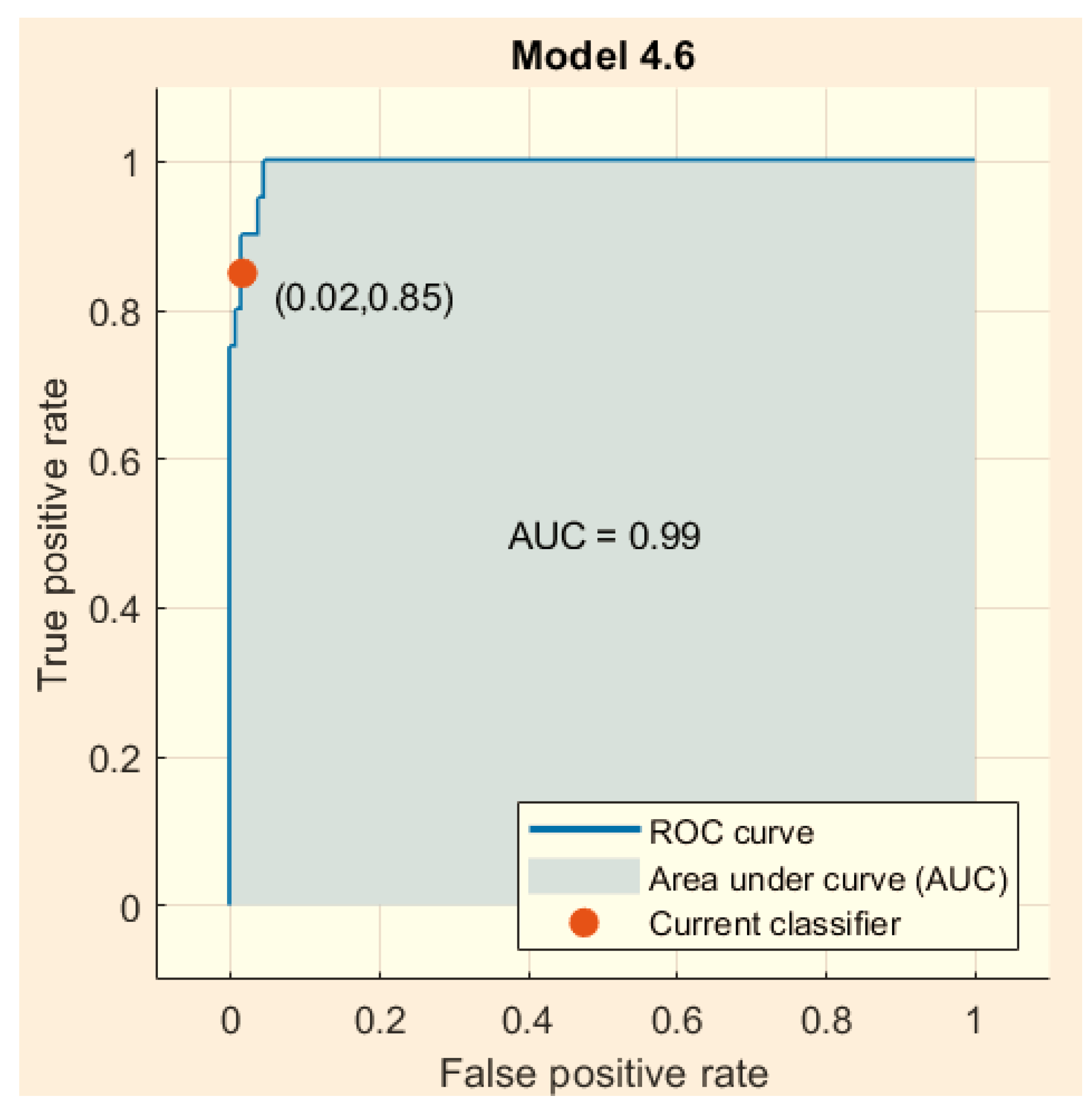
Figure 5 shows that the predicted class 1, referring to the excellent class, appeared 19 times; 17/19 is a correct prediction class (89%), and 11% (2/19) occurred with class 2 (good state). The receiver operating characteristic (ROC) is illustrated for class 1 in Figure 6. The marker on ROC presents the current classifier performance where the false positive rate (FPR) is on the x-axis, and the true positive rate (TPR) is on the y-axis.
Figure 6 explained that the FPR is 0.02, i.e., 2% of the data samples were assigned incorrectly to the positive class. The TPR refers to 0.85, which explains that the classifier correctly assigns 88% of the samples to the positive class. Right angle for ROC refers to perfect classifying results. When the angle is 45°, it shows a poor classification result. The area under the curve (AUC) showed the overall accuracy of the classifier for the class. Larger AUC values refer to better classifier performance. Figure 6 explains that the AUC is 99%, which refers to better classifying.
Table 6 shows 18 samples (randomly selected) where the chemical values gathered are shown in the left rows. The water quality index (WQI) and the quality achieved for the samples are shown in the following columns and finally, the SVM model prediction is depicted in the right column. The classification accuracy is 88.9% (16/18) due to two of the samples being wrong diagnosed (Sample 1 and sample 17).

3.4. Results with Standardization of the Data [(X − μ)/σ] Linear SVM

The standardization process of the data has been carried out following Equation (3). Again, linear SVM is obtained as the best classification tool, with a prediction accuracy of 95.4%. Figure 7 indicates that standardization of the raw data only enhanced the prediction accuracy of the excellent state (18/20; 90% accuracy). On the other hand, all other states are equal to those obtained with raw data. Therefore, the prediction accuracy of the test data samples was the same as that of the raw data.
The k-fold cross-validation was used to check the robustness of the constructed model for developing high accuracy classification. Tenfold cross-validation is used, which divides the data into two groups (80% of the data samples for training, and the remaining 20% is for the testing process). These processes were repeated ten times with a random collection of the samples. Then the average of the classification accuracy was determined. Standardizing the data samples slightly enhanced the training classification accuracy to 95.4% compared with 94.7% using the raw data. The testing results’ classification accuracy shows that the constructed classification model is so beneficial to reduce the time needed to compute the WQI for each sample. The data of new samples are used as input data, and the WQI is directly identified.

4. Discussion

Table 3 shows that concentrations of Calcium experienced varied considerably from 12.0 to 832.0 mg/L (average value 137.69 mg/L). These values are much higher than the standards in Europe for Calcium in drinking water ranging from 75–200 mg/L [56]. Moreover, concentrations of Magnesium also varied considerably from 3.0 to 560.0 mg/L (average value of 76.03 mg/L). These values are much higher than other reference values found in literature as 78–155 mg/L (Calcium) and 28–54 mg/L (Magnesium) found in Slovakia [58] and also in Egypt, as 8–197 mg/L (Calcium) and 1.6–110 mg/L (Magnesium) [59].
Moreover, Table 3 also depicts strong variations in sodium levels of groundwater samples. The values ranged from 5.0 mg/L to 2967.0 mg/L (186.4 mg/L as average value) and an extremally variable coefficient of variation of 169.17%. Similar values (22.15–2769.5 mg/L) were found in Ghana [60] or south Africa (48–6971 mg/L) [61]. In the present study, the potassium concentration observed ranged between 1.00 to 59.0 mg/L, being these values lower than the identified in some studies carried out in Ghana (0.21–126 mg/L) [62]. The chloride concentration variation was 10–443 mg/L, while values higher to 21–110 mg/L were observed in Tunisia [63]. Sulfates concentration ranges between 38–2370 mg/L (average 376.78 mg/L) and nitrates also vary considerably from 1.0 to 390.0 mg/L (with a mean value of 26.82 mg/L) being aware that limits for drinking water are 10 mg/L in the United States and 50 mg/L according to World Health Organization [56].
The bicarbonates values in the water sampling points in our study area are between 20 and 529 mg/L, and electrical conductivity and mineralization varied considerably from 290 (µδ/cm) to 8660 (µδ/cm) and 186 mg/L to 5493 mg/L, respectively.
At different water quality levels, pH levels varied considerably from 6.58 to 10.60, spanning one order of magnitude with a mean value of 7.71 and a coefficient of variation of 6.64%. These values are not in agreement with the permissible limits (6.5–8.5 mg/L) for drinking water proposed by the World Health Organization [56].
The result shown in Table 4 revealed that 14.8% of samples fell into the excellent category (Class I; with values ranging from 33.32 to 49.48), 62.7% were classed as good (Class II; values varied from 50.9 to 99.26), 17.2% in the poor category (Class III, 100.15 to 183.82), and 5.3% are unsafe for drinking (Class IV values varied from 202.9 to 365.7). Being aware that 75% of water comes from groundwater [64] and considering the huge amount of data required to calculate WQI. Authors have found better values for predicting WQI using the SVM model than other approaches in Malaysia with the coefficient of determination (R2) equal to 0.8796 [64], or R2 = 0.9 also in Malaysia [65] using LSSVM (Least square SVM), and R2 = 0.87 in Iran [66]. However, other better results were found in Poland, where authors obtained R2 = 0.99 using neural networks [67]. Similar trustworthy results were achieved in Ethiopia, Vietnam and Brazil among others [68,69,70,71].

5. Conclusions

In order to maintain the availability of resources for drinkable water and to monitor pollution, the prediction of water quality indexes is extremely important. Thus, planning and managing water resources can greatly benefit from precise groundwater level predictions. As a result, an effort is made in this work to create a forecasting model that is effective for predicting groundwater quality by using the water quality index (WQI) in the Wilaya of Naama, placed in the southwestern region of Algeria. Based on many characteristics and indexes, conventional approaches evaluate water suitability for drinking and domestic purposes. Although these techniques are reliable tools, they can be costly and time-consuming. Therefore, this study proposes an alternative machine learning method for predicting water quality using only a few simple water quality criteria. The data used to conduct the study were collected from 169 samples of groundwater from 12 municipalities in the Wilaya of Naâma. A set of representative supervised machine learning algorithms has been used to estimate the WQI indicator. Based on WQI results, four classes were fixed: excellent, good, poor, and very poor or unsafe water. A relevant percentage (62.7%) of the considered physicochemical parameters depicted good water quality results. Related to prediction tools, main results showed that Support Vector Machine (SVM) algorithms classify groundwater quality with high accuracy (95.4%) with standardized data and lower accuracy (88.88%) for raw data. Therefore, a great correlation between observed and predicted water quality data was obtained in the present manuscript. These results offer a useful performance assessment tool for decision-makers, and further investigation can be undertaken by integrating the findings of this research on a large scale in arid areas. In conclusion, the SVM model is a simple and effective empirical model to simulate water quality, and the method presented in this work is sufficiently general to be applied to a wide range of arid areas.

Author Contributions

Conceptualization, A.D.; data curation, A.D.; formal analysis, A.D., A.J.-A., S.S.M.G. and E.E.H.; funding acquisition, A.J.-A., M.Á.P. and S.S.M.G.; investigation, A.D., A.J.-A., M.Á.P. and S.S.M.G.; methodology, A.D., A.J.-A., M.Á.P., S.S.M.G. and E.E.H.; project administration, A.D., A.J.-A., M.Á.P., S.S.M.G. and E.E.H.; resources, A.D.; software, A.D. and S.S.M.G.; supervision, A.D., A.J.-A., M.Á.P., S.S.M.G. and E.E.H.; validation, S.S.M.G.; visualization, A.D., A.J.-A., M.Á.P. and E.E.H.; writing—original draft, A.D., A.J.-A., M.Á.P., S.S.M.G. and E.E.H.; writing—review and editing, A.D., A.J.-A., M.Á.P., S.S.M.G. and E.E.H. All authors have read and agreed to the published version of the manuscript.

Funding

This research received funding from Taif University Researchers Supporting Project TURSP 2020/34, Taif University, Taif, Saudi Arabia.

Institutional Review Board Statement

Not applicable.

Informed Consent Statement

Not applicable.

Data Availability Statement

Not applicable.

Acknowledgments

This work is part of PRFU project N° E04N01CU450120220001. The authors gratefully acknowledge the support of the General Directorate of Scientific Research and Technological Development (DGRSDT) and to Taif University Researchers Supporting Project TURSP 2020/34, Taif University, Taif, Saudi Arabia.

Conflicts of Interest

The authors declare no conflict of interest.

References

  1. Keesstra, S.D.; Geissen, V.; Mosse, K.; Piiranen, S.; Scudiero, E.; Leistra, M.; van Schaik, L. Soil as a filter for groundwater quality. J. Curr. Opin. Environ. Sustain. 2012, 4, 507–516. [Google Scholar] [CrossRef]
  2. Pulido, M.; Barrena-González, J.; Alfonso-Torreño, A.; Robina-Ramírez, R.; Keesstra, S. The problem of water use in rural areas of Southwestern Spain: A local perspective. Water 2019, 11, 1311. [Google Scholar] [CrossRef]
  3. Zubaidi, S.L.; Ortega-Martorell, S.; Al-Bugharbee, H.; Olier, I.; Hashim, K.S.; Gharghan, S.K.; Kot, P.; Al-Khaddar, R. Urban water demand prediction for a city that suffers from climate change and population growth: Gauteng province case study. Water 2020, 12, 1885. [Google Scholar] [CrossRef]
  4. WHO. UN-Water Global Analysis and Assessment of Sanitation and Drinking-Water (GLAAS) 2014 in Report: Investing in Water and Sanitation: Increasing Access, Reducing Inequalities; World Health Organization: Geneva, Switzerland, 2014.
  5. Sorenson, S.B.; Morssink, C.; Campos, P.A. Safe access to safe water in low income countries: Water fetching in current times. Soc. Sci. Med. 2011, 72, 1522–1526. [Google Scholar] [CrossRef] [PubMed]
  6. Downing, J.A.; Polasky, S.; Olmstead, S.M.; Newbold, S.C. Protecting local water quality has global benefits. Nat. Commun. 2021, 12, 2709. [Google Scholar] [CrossRef] [PubMed]
  7. Luvhimbi, N.; Tshitangano, T.G.; Mabunda, J.T.; Olaniyi, F.C.; Edokpayi, J.N. Water quality assessment and evaluation of human health risk of drinking water from source to point of use at Thulamela municipality, Limpopo Province. Sci. Rep. 2022, 12, 6059. [Google Scholar] [CrossRef]
  8. Uddin, G.; Nash, S.; Olbert, A.I. A review of water quality index models and their use for assessing surface water quality. Ecol. Indic. 2020, 122, 107218. [Google Scholar] [CrossRef]
  9. Lumb, A.; Sharma, T.C.; Bibeault, J.-F. A review of genesis and evolution of water quality index (WQI) and some future directions. Water Qual. Expo. Health 2011, 3, 11–24. [Google Scholar] [CrossRef]
  10. Zhang, Q.; Xu, P.; Qian, H. Groundwater quality assessment using improved water quality index (WQI) and human health risk (HHR) evaluation in a semi-arid region of northwest China. Expo. Health 2020, 12, 487–500. [Google Scholar] [CrossRef]
  11. Akter, T.; Jhohura, F.T.; Akter, F.; Chowdhury, T.R.; Mistry, S.K.; Dey, D.; Barua, M.K.; Islam, A.; Rahman, M. Water Quality Index for measuring drinking water quality in rural Bangladesh: A cross-sectional study. J. Health Popul. Nutr. 2016, 35, 4. [Google Scholar] [CrossRef] [Green Version]
  12. Abba, S.I.; Pham, Q.B.; Saini, G.; Linh, N.T.T.; Ahmed, A.N.; Mohajane, M.; Khaledian, M.; Abdulkadir, R.A.; Bach, Q.-V. Implementation of data intelligence models coupled with ensemble machine learning for prediction of water quality index. Environ. Sci. Pollut. Res. 2020, 27, 41524–41539. [Google Scholar] [CrossRef]
  13. Mohammadpour, R.; Shaharuddin, S.; Chang, C.K.; Zakaria, N.A.; Ab Ghani, A.; Chan, N.W. Prediction of water quality index in constructed wetlands using support vector machine. Environ. Sci. Pollut. Res. 2014, 22, 6208–6219. [Google Scholar] [CrossRef]
  14. Singh, K.P.; Basant, N.; Gupta, S. Support vector machines in water quality management. Anal. Chim. Acta 2011, 703, 152–162. [Google Scholar] [CrossRef]
  15. Safavi, H.R.; Esmikhani, M. Conjunctive use of surface water and groundwater: Application of support vector machines (SVMs) and genetic algorithms. Water Resour. Manag. 2013, 27, 2623–2644. [Google Scholar] [CrossRef]
  16. Gakii, C.; Jepkoech, J. A classification model for water quality analysis using decision tree. Eur. J. Comput. Sci. Inf. Technol. 2019, 7, 1–8. [Google Scholar]
  17. Jeihouni, M.; Toomanian, A.; Mansourian, A. Decision tree-based data mining and rule induction for identifying high quality groundwater zones to water supply management: A novel hybrid use of data mining and GIS. Water Resour. Manag. 2019, 34, 139–154. [Google Scholar] [CrossRef]
  18. Chen, K.; Chen, H.; Zhou, C.; Huang, Y.; Qi, X.; Shen, R.; Liu, F.; Zuo, M.; Zou, X.; Wang, J.; et al. Comparative analysis of surface water quality prediction performance and identification of key water parameters using different machine learning models based on big data. Water Res. 2019, 171, 115454. [Google Scholar] [CrossRef]
  19. Zhang, C.; Ma, Y. Ensemble Machine Learning: Methods and Applications; Springer: Berlin/Heidelberg, Germany, 2012. [Google Scholar]
  20. Xin, X.; Lu, W.-X.; Gong, L. Discriminant analysis method application in water quality assessment: Take Yinma River as example. In Proceedings of the 2010 4th International Conference on Bioinformatics and Biomedical Engineering, Chengdu, China, 18–20 June 2010. [Google Scholar]
  21. Lei, L. Assessment of Water Quality Using Multivariate Statistical Techniques in the Ying River Basin, China. Master Thesis, University of Michigan, Ann Arbor, MI, USA, April 2014. Available online: https://deepblue.lib.umich.edu/bitstream/handle/2027.42/106539/final%20draft_Lei%20Lei.pdf?sequence= (accessed on 29 July 2022).
  22. Al-Adhaileh, M.H.; Alsaade, F.W. Modelling and prediction of water quality by using artificial intelligence. Sustainability 2021, 13, 4259. [Google Scholar] [CrossRef]
  23. Li, Y.; Khan, M.Y.A.; Jiang, Y.; Tian, F.; Liao, W.; Fu, S.; He, C. CART and PSO+KNN algorithms to estimate the impact of water level change on water quality in Poyang Lake, China. Arab. J. Geosci. 2019, 12, 287. [Google Scholar] [CrossRef]
  24. Egbueri, J.C.; Agbasi, J.C. Data-driven soft computing modeling of groundwater quality parameters in southeast Nigeria: Comparing the performances of different algorithms. Environ. Sci. Pollut. Res. 2022, 29, 38346–38373. [Google Scholar] [CrossRef]
  25. Pham, T.L.; Tran, T.H.Y.; Tran, T.T.; Ngo, X.Q.; Nguyen, X.D. Assessment of surface water quality in a drinking water supply reservoir in Vietnam: A combination of different indicators. Rend. Lincei. Sci. Fis. E Nat. 2022, 1–10. Available online: https://link.springer.com/article/10.1007/s12210-022-01086-5 (accessed on 29 July 2022). [CrossRef]
  26. He, B.; Shi, Y.; Wan, Q.; Zhao, X. Prediction of customer attrition of commercial banks based on SVM model. Procedia Comput. Sci. 2014, 31, 423–430. [Google Scholar] [CrossRef]
  27. Samantaray, S.; Sahoo, A.; Ghose, D.K. Assessment of sediment load concentration using SVM, SVM-FFA and PSR-SVM-FFA in arid watershed, India: A Case Study. KSCE J. Civ. Eng. 2020, 24, 1944–1957. [Google Scholar] [CrossRef]
  28. Kurniawan, I.; Hayder, G.; Mustafa, H.M. Predicting water quality parameters in a complex river system. J. Ecol. Eng. 2021, 22, 250–257. [Google Scholar] [CrossRef]
  29. Koranga, M.; Pant, P.; Pant, D.; Bhatt, A.K.; Pant, R.P.; Ram, M.; Kumar, T. SVM Model to Predict the Water Quality Based on Physicochemical Parameters. Int. J. Math. Eng. Manag. Sci. 2021, 6, 645–659. [Google Scholar] [CrossRef]
  30. Tan, G.; Yan, J.; Gao, C.; Yang, S. Prediction of water quality time series data based on least squares support vector machine. Procedia Eng. 2012, 31, 1194–1199. [Google Scholar] [CrossRef]
  31. Ladjal, M.; Bouamar, M.; Djerioui, M.; Brik, Y. Performance evaluation of ANN and SVM multiclass models for intelligent water quality classification using Dempster-Shafer Theory. In Proceedings of the 2016 International Conference on Electrical and Information Technologies (ICEIT), Tangiers, Morocco, 4–7 May 2016. [Google Scholar]
  32. Kouadri, S.; Elbeltagi, A.; Islam, A.R.M.T.; Kateb, S. Performance of machine learning methods in predicting water quality index based on irregular data set: Application on Illizi region (Algerian southeast). Appl. Water Sci. 2021, 11, 190. [Google Scholar] [CrossRef]
  33. Boudibi, S.; Sakaa, B.; Benguega, Z.; Fadlaoui, H.; Othman, T.; Bouzidi, N. Spatial prediction and modeling of soil salinity using simple cokriging, artificial neural networks, and support vector machines in El Outaya plain, Biskra, southeastern Algeria. Acta Geochim. 2021, 40, 390–408. [Google Scholar] [CrossRef]
  34. Dilmi, S.; Ladjal, M. A novel approach for water quality classification based on the integration of deep learning and feature extraction techniques. Chemom. Intell. Lab. Syst. 2021, 214, 104329. [Google Scholar] [CrossRef]
  35. Ghoneim, S. Determination of Transformers’ Insulating Paper State Based on Classification Techniques. Processes 2021, 9, 427. [Google Scholar] [CrossRef]
  36. Bouarfa, S.; Bellal, S.A. Assessment of the Aeolian sand dynamics in the region of Ain Sefra (Western Algeria), using wind data and satellite imagery. Arab. J. Geosci. 2018, 11, 56. [Google Scholar] [CrossRef]
  37. Hadjadj, K.; Guerine, L.; Derdour, A. Flore des populations de frêne dimorphe (fraxinus dimorpha coss. & durieu) dans l’Atlas Saharien (Monts des Ksours, Algérie). J. Lejeunia Rev. De Bot. 2021. [Google Scholar] [CrossRef]
  38. Derdour, A.; Guerine, l.; Allali, M. Assessment of drinking and irrigation water quality using WQI and SAR method in Maâder sub-basin, Ksour Mountains, Algeria. J. Sustain. Water Resour. Manag. 2021, 7, 8. [Google Scholar] [CrossRef]
  39. Derdour, A.; Ali, M.M.M.; Sari, S.M.C. Evaluation of the quality of groundwater for its appropriateness for drinking purposes in the watershed of Naama, SW of Algeria, by using water quality index (WQI). SN Appl. Sci. 2020, 2, 1951. [Google Scholar] [CrossRef]
  40. Benaradj, A.; Boucherit, H.; Merzougui, T. Water Resources, State of Play, and Development Prospects in the Steppe Region of Naâma (Western Algeria), in Water Resources in Algeria-Part II; Springer: Berlin/Heidelberg, Germany, 2020; pp. 253–283. [Google Scholar]
  41. Derdour, A.; Bouanani, A. Coupling HEC-RAS and HEC-HMS in rainfall–runoff modeling and evaluating floodplain inundation maps in arid environments: Case study of Ain Sefra city, Ksour Mountain. SW of Algeria. Environ. Earth Sci. 2019, 78, 586. [Google Scholar]
  42. Guerine, L.; Belgourari, M.; Guerinik, H. Cartography and diachronic study of the naama sabkha (Southwestern Algeria) remotely sensed vegetation index and soil properties. J. Rangel. Sci. 2020, 10, 172–187. [Google Scholar]
  43. Rahmani, A.; Bouanani, A.; Kacemi, A.; Hamed, K.B. Contribution of GIS for the survey and the management of water resources in the basin “Benhandjir–Tirkount” (Ain Sefra)–mounts of Ksour-Saharian Atlas–Algeria. J. Fundam. Appl. Sci. 2017, 9, 829–846. [Google Scholar] [CrossRef]
  44. Varol, S.; Davraz, A. Evaluation of the groundwater quality with WQI (Water Quality Index) and multivariate analysis: A case study of the Tefenni plain (Burdur/Turkey). Environ. Earth Sci. 2014, 73, 1725–1744. [Google Scholar] [CrossRef]
  45. Bora, M.; Goswami, D.C. Water quality assessment in terms of water quality index (WQI): Case study of the Kolong River, Assam, India. Appl. Water Sci. 2016, 7, 3125–3135. [Google Scholar] [CrossRef]
  46. Ramakrishnaiah, C.R.; Sadashivaiah, C.; Ranganna, G. Assessment of water quality index for the groundwater In Tumkur Taluk, Karnataka State, India. E J. Chem. 2009, 6, 523–530. [Google Scholar] [CrossRef]
  47. Hassan, A.N.; El-Hag, A. Two-layer ensemble-based soft voting classifier for transformer oil interfacial tension prediction. Energies 2020, 13, 1735. [Google Scholar] [CrossRef]
  48. Liu, Y.; Li, J.; Qiao, L.; Chen, S.; Liu, S.; Liu, J. Fault diagnosis of power transformer based on tree ensemble model. IOP Conf. Ser. Mater. Sci. Eng. 2020, 715, 012032. [Google Scholar] [CrossRef]
  49. Kherif, O.; Benmahamed, Y.; Teguar, M.; Boubakeur, A.; Ghoneim, S.S.M. accuracy improvement of power transformer faults diagnostic using KNN classifier with decision tree principle. IEEE Access 2021, 9, 81693–81701. [Google Scholar] [CrossRef]
  50. Silva, A.; Stam, A. Discriminant Analysis; Reading and understanding multivariate statistics; Grimm, L.G., Yarnold, P.R., Eds.; APA Books: Washington, DC, USA, 1995; pp. 277–318. [Google Scholar]
  51. Yazdani-Asrami, M.; Taghipour-Gorjikolaie, M.; Song, W.; Zhang, M.; Yuan, W. Prediction of nonsinusoidal AC loss of superconducting tapes using artificial intelligence-based models. IEEE Access 2020, 8, 207287–207297. [Google Scholar] [CrossRef]
  52. Benmahamed, Y.; Kherif, O.; Teguar, M.; Boubakeur, A.; Ghoneim, S. Accuracy improvement of transformer faults diagnostic based on DGA data using SVM-BA classifier. Energies 2021, 14, 2970. [Google Scholar] [CrossRef]
  53. Zhang, Y.; Li, J.; Fan, X.; Liu, J.; Zhang, H. Moisture prediction of transformer oil-immersed polymer insulation by applying a support vector machine combined with a genetic algorithm. Polymers 2020, 12, 1579. [Google Scholar] [CrossRef] [PubMed]
  54. Liu, T.; Zhu, X.; Pedrycz, W.; Li, Z. A design of information granule-based under-sampling method in imbalanced data classification. Soft Comput. 2020, 24, 17333–17347. [Google Scholar] [CrossRef]
  55. Tharwat, A.; Hassanien, A.E.; Elnaghi, B.E. A BA-based algorithm for parameter optimization of Support Vector Machine. Pattern Recognit. Lett. 2017, 93, 13–22. [Google Scholar] [CrossRef]
  56. WHO (World Health Organization). Guidelines for Drinking-Water Quality: First Addendum to the Fourth Edition; World Health Organization: Geneva, Switzerland, 2017.
  57. Taha, I.B.; Mansour, D.-E.A.; Ghoneim, S.S.; Elkalashy, N.I. Conditional probability-based interpretation of dissolved gas analysis for transformer incipient faults. IET Gener. Transm. Distrib. 2017, 11, 943–951. [Google Scholar] [CrossRef]
  58. Rapant, S.; Cvečková, V.; Fajčíková, K.; Sedláková, D.; Stehlíková, B. Impact of calcium and magnesium in groundwater and drinking water on the health of inhabitants of the Slovak Republic. Int. J. Environ. Res. Public Health 2017, 14, 278. [Google Scholar] [CrossRef]
  59. Ismail, E.; Abdelhalim, A.; Heleika, M.A. Hydrochemical characteristics and quality assessment of groundwater aquifers northwest of Assiut District, Egypt. J. Afr. Earth Sci. 2021, 181, 104260. [Google Scholar] [CrossRef]
  60. Ganyaglo, S.Y.; Gibrilla, A.; Teye, E.M.; Owusu-Ansah, E.D.-G.J.; Tettey, S.; Diabene, P.Y.; Asimah, S. Groundwater fluoride contamination and probabilistic health risk assessment in fluoride endemic areas of the Upper East Region, Ghana. Chemosphere 2019, 233, 862–872. [Google Scholar] [CrossRef]
  61. Ntanganedzeni, B.; Elumalai, V.; Rajmohan, N. Coastal aquifer contamination and geochemical processes evaluation in tugela catchment, South Africa—Geochemical and statistical approaches. Water 2018, 10, 687. [Google Scholar] [CrossRef] [Green Version]
  62. Osiakwan, G.M.; Appiah-Adjei, E.K.; Kabo-Bah, A.T.; Gibrilla, A.; Anornu, G. Assessment of groundwater quality and the controlling factors in coastal aquifers of Ghana: An integrated statistical, geostatistical and hydrogeochemical approach. J. Afr. Earth Sci. 2021, 184, 104371. [Google Scholar] [CrossRef]
  63. Dassi, L. Use of chloride mass balance and tritium data for estimation of groundwater recharge and renewal rate in an unconfined aquifer from North Africa: A case study from Tunisia. Environ. Earth Sci. 2010, 60, 861–871. [Google Scholar] [CrossRef]
  64. Leong, W.C.; Bahadori, A.; Zhang, J.; Ahmad, Z. Prediction of water quality index (WQI) using support vector machine (SVM) and least square-support vector machine (LS-SVM). Int. J. River Basin Manag. 2019, 19, 149–156. [Google Scholar] [CrossRef]
  65. Chia, S.L.; Chia, M.Y.; Koo, C.H.; Huang, Y.F. Integration of advanced optimization algorithms into least-square support vector machine (LSSVM) for water quality index prediction. Water Supply 2021, 22, 1951–1963. [Google Scholar] [CrossRef]
  66. Kamyab-Talesh, F.; Mousavi, S.-F.; Khaledian, M.; Yousefi-Falakdehi, O.; Norouzi-Masir, M. Prediction of water quality index by support vector machine: A case study in the Sefidrud Basin, Northern Iran. Water Resour. 2019, 46, 112–116. [Google Scholar] [CrossRef]
  67. Kulisz, M.; Kujawska, J.; Przysucha, B.; Cel, W. Forecasting water quality index in groundwater using artificial neural network. Energies 2021, 14, 5875. [Google Scholar] [CrossRef]
  68. Abera, K.A.; Gebreyohannes, T.; Abrha, B.; Hagos, M.; Berhane, G.; Hussien, A.; Belay, A.S.; Van Camp, M.; Walraevens, K. Vulnerability Mapping of Groundwater Resources of Mekelle City and Surroundings, Tigray Region, Ethiopia. Water 2022, 14, 2577. [Google Scholar] [CrossRef]
  69. Giao, N.T.; Dan, T.H.; Van Ni, D.; Anh, P.K.; Nhien, H.T.H. Spatiotemporal Variations in Physicochemical and Biological Properties of Surface Water Using Statistical Analyses in Vinh Long Province, Vietnam. Water 2022, 14, 2200. [Google Scholar] [CrossRef]
  70. Abuzaid, A.S.; Jahin, H.S. Combinations of multivariate statistical analysis and analytical hierarchical process for indexing surface water quality under arid conditions. J. Contam. Hydrol. 2022, 248, 104005. [Google Scholar] [CrossRef] [PubMed]
  71. Braga, F.H.R.; Dutra, M.L.S.; Lima, N.S.; Silva, G.M.; Miranda, R.C.M.; Firmo, W.C.A.; Moura, A.R.L.; Monteiro, A.S.; Silva, L.C.N.; Silva, D.F.; et al. Study of the Influence of Physicochemical Parameters on the Water Quality Index (WQI) in the Maranhão Amazon, Brazil. Water 2022, 14, 1546. [Google Scholar] [CrossRef]
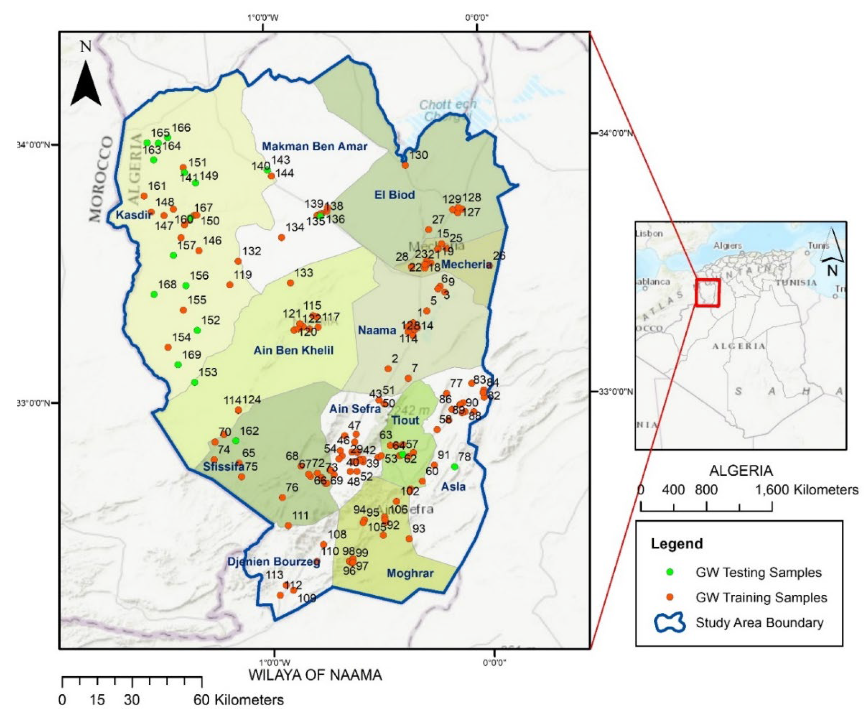
Figure 1. Localization of the study area and sampling points.
Water 14 02801 g001
Figure 2. SVM algorithm indicates the margin separating two classes.
Water 14 02801 g002
Figure 3. Spatial distribution of WQI in the study area.
Water 14 02801 g003
Figure 4. Confusion matrix of linear SVM that was applied to the raw data, (Green refers to True Positive, red refers to False negative) (a) corrected prediction samples for each class (b) prediction accuracy of each class.
Water 14 02801 g004
Figure 5. Positive–negative predictive values of linear SVM confusion matrix of Raw data, (Green refers to True Positive, red refers to False negative).
Water 14 02801 g005
Figure 6. The ROC result of the ensemble bagged tree.
Water 14 02801 g006
Figure 7. Confusion matrix of linear SVM that was applied to the standardization data (Green refers to True Positive, red refers to False negative) (a) corrected prediction samples for each class (b) prediction accuracy of each class.
Water 14 02801 g007
Table 1. The weighting of each physicochemical parameter.
PC-ParametersUnitsPermissible LimitsWeight (Wi)Relative Weight (Wi)
pH 8.540.118
Electrical Conductivityµδ/cm280040.118
Mineralizationmg/L200040.118
Magnesiummg/L5010.029
Calciummg/L20020.059
Potassiummg/L1220.059
Sodiummg/L20020.059
Chloridesmg/L50030.088
Sulphatesmg/L40040.118
Nitratesmg/L5050.147
Bicarbonatesmg/L12030.088
341
Table 2. Distribution of the training and testing samples according to the WQI class.
SamplesExcellent (1)Good (2)Poor (3)Very Poor or Unsafe (4)Total
Training20101246151
Testing555318
Total25106299169
Table 3. Descriptive statistics of groundwater parameters of the Wilaya of Naâma.
Min ValueMax ValueMean ValueStandard Values [56]Standard DeviationCoefficient of Variation (%)
Ca++12.00832.00137.6975–200122.5088.97
Mg++3.00560.0076.035068.8590.56
Na+5.002967.00186.40200315.33169.17
K+1.0059.008.97128.4794.38
Cl10.00443.00118.9525062.9052.88
SO42−38.002370.00376.78250437.83116.20
HCO320.00529.00237.8512063.9226.87
NO31.00390.0026.825036.85137.40
Cond.290.008660.001556.8215001306.6083.93
Miner.186.005493.001076.67-877.3081.48
pH6.5810.607.716.5–8.50.516.64
Table 4. Summary of WQI evaluation in the Wilaya of Naâma.
ClassesTypeNumber of Samples%
IExcellent2514.8
IIGood10662.7
IIIPoor2917.2
IVUnsafe95.3
Table 5. Comparison between different classifiers.
ClassifierTraining Data
Raw DataStandardization
1. Decision Tree (DT)
Fine tree83.475.5
Medium tree83.475.5
Coarse tree81.576.8
Linear discriminant88.788.7
Quadratic discriminantFailFail
2. Support Vector Machine (SVM)
Linear SVM94.795.4
Quadratic SVM93.493.4
Cubic SVM90.791.4
Fine Gaussian SVM66.967.5
Medium Gaussian SVM90.191.1
Coarse Gaussian SVM74.874.2
3. K-Nearest Neighbors (KNN)
Fine KNN86.184.1
Medium KNN81.583.4
Coarse KNN66.966.9
Cosine KNN72.878.8
Cubic KNN80.880.1
Weighted KNN83.484.1
4. Ensemble Trees
Ensemble boosted trees66.966.9
Ensemble bagged trees86.888.1
Ensemble subspace Discriminant83.483.4
Ensemble subspace KNN82.888.7
Ensemble RUSBoosted trees75.578.8
5. Discrimination Analysis (DA)
Linear Discrimination90.7%90.1
Quadratic Discrimination FailedFailed
Table 6. The prediction results of the 18 testing samples with linear SVM.
Ca++Mg++Na+K+ClSO4HCO3NO3Cond.Miner.pHWQI ResultsQualityPred.
7246554104154173109006188.449.48ExcellentGood
59504446118422347605447.2748.44ExcellentExcellent
3329163216416932902237.6733.32ExcellentExcellent
723248363136224177125107.3749.66ExcellentExcellent
68284645613219875874207.3943.62ExcellentExcellent
606832241501722716198015037.3280.06GoodGood
118647431422282582711869007.5367.70GoodGood
735941278219217128676587.3452.77GoodGood
116483723636320389457177.2255.10GoodGood
91563549914628448906766.9454.36GoodGood
1019944417139.69081068273020737.34108.02PoorPoor
12812431112152.554620110247018757.5100.95PoorPoor
50629014019184237011339352026727.34178.91PoorPoor
22215912011205102019325205015567.29107.86PoorPoor
3032118512116149517334229017387.25128.38PoorPoor
112.233147219265.8153618244460028528241.26Very PoorVery Poor
4519512773820013201271640039688.1220.54Very PoorPoor
16045297826.1172.118722889620052708365.72Very PoorVery Poor
Publisher’s Note: MDPI stays neutral with regard to jurisdictional claims in published maps and institutional affiliations.