Article

Where You Drink Water: An Assessment of the Tennessee, USA Public Water Supply

by
Ke Jack Ding
1,*,
George M. Hornberger
2,
Elaine L. Hill
3,4,5 and
Yolanda J. McDonald
6,*
1
Department of Civil and Environmental Engineering, Vanderbilt University, Nashville, TN 37235, USA
2
Department of and Environmental Civil Engineering, Vanderbilt University, Nashville, TN 37235, USA
3
Department of Public Health Sciences, University of Rochester Medical Center, Rochester, NY 14642, USA
4
Department of Economics, University of Rochester Medical Center, Rochester, NY 14642, USA
5
Department of Obstetrics and Gynecology, University of Rochester Medical Center, Rochester, NY 14642, USA
6
Department of Human and Organizational Development, Vanderbilt University, Nashville, TN 37235, USA
*
Authors to whom correspondence should be addressed.
Water 2022, 14(16), 2562; https://doi.org/10.3390/w14162562
Submission received: 14 June 2022 / Revised: 15 August 2022 / Accepted: 16 August 2022 / Published: 20 August 2022
(This article belongs to the Special Issue Drinking Water: Water Quality and Treatment)

Abstract

:
Monitoring drinking water quality is essential to protect people’s health and wellbeing. In the United States, the Safe Drinking Water Information System (SDWIS) database records the occurrence of a drinking water violation regulation in public water systems. A notable shortcoming of SDWIS is the lack of the contaminant concentration level about the allowable maximum contaminant threshold. In this study, we take advantage of both the SDWIS violation database and the contaminants sampling database at the state level to examine the drinking water quality of all kinds of drinking water systems in detail. We obtained sampling data (i.e., the concentration level of contaminants) of public water systems (PWSs) in Tennessee and explored the statistical distribution of contaminant concentration data in relation to the enforceable maximum regulatory contaminant level). We use both SDWIS violation records and actual concentrations of contaminants from the sampling data to study the factors that influence the drinking water quality of PWSs. We find that different types of violations were more frequent in (1) specific geological regions, (2) counties with PWSs that serve a larger population (10,000 to 100,000 people), and (3) places with abundant surface water, such as near a lake or major river. Additionally, the distribution of measured concentrations for many contaminants was not smooth but was punctuated by discontinuities at selected levels, such as at 50% of the maximum contaminant level. Such anomalies in the sampling data do not indicate violations, but more investigation is needed to determine the reasons behind the punctuated changes.

1. Introduction

In the United States, 90% of the population receives piped water from public water systems (PWSs). The Safe Drinking Water Act (SWDA), passed in 1974 and amended in 1986 and 1996, is the federal statute that regulates public water systems (PWSs) to protect the health and wellbeing of people. A PWS provides water for human consumption to 15 or more service connections or at least 25 people for 60 or more days a year. Despite regulatory guidelines per the SWDA, drinking water quality issues continue to occur that could have adverse health effects [1,2].
The United States Environmental Protection Agency (USEPA) is mandated to enforce federal SDWA regulations. A state can apply to the USEPA for primacy status. At a minimum, an entity must adhere to federal SDWA regulations to be granted primacy status. Primacy enables state agencies to have direct regulatory oversight of PWS drinking water: some states enforce more stringent standards than the federal guidelines. PWSs report drinking water quality violations to primacy agencies, and then these data are uploaded to the USEPA’s Safe Drinking Water Information System (SDWIS).
There has been extensive research that focused on the drinking water quality (e.g., violations) of US community water systems (one of three types of public water systems that provides water to the same population all year, CWS hereafter). Violation categories are defined as exceedance of (1) exceedance of Maximum Contaminant Level [MCL]; (2) exceedance of Treatment Technique [TT]; (3) exceedance of Maximum Residual Disinfectant Level [MRDL] threshold; (4) monitoring [MON]; (5) reporting [RPT]; (6) public note [PN]; or (7) Other per the 2019 Safe Drinking Water Information System (SDWIS) Federal Reporting Services definitions. Using 2011 SDWIS data, Rubin [2] found negligible differences comparing small (i.e., serving less than 3300 persons) to large (i.e., serving 10,001 to 100,000 persons) CWSs percentage of health-based violations. However, small compared to large CWSs were more likely to report MON and RPT violations. Health-based violations were slightly more likely in CWSs relying on surface water than groundwater; no differences in source water in MON and RPT violations (21]. Allaire et al. [1] constructed a panel dataset from 1982 to 2015 using SDWIS to study the trends of health-based violations for CWSs. They found that health-based violations in the Southwest have been increasing over time and urban areas tend to have fewer violations than rural areas. McDonald and Jones [3] used SDWIS data from 2011 to 2015 to assess the association between county-level race/ethnicity and socioeconomic status characteristics and CWS violations (i.e., all categories) aggregated at the county level. Findings showed that communities in counties with a higher percentage of minorities and residents with lower socioeconomic status were more likely to experience drinking water violations, regardless of the size of the CWSs. Eskaf [4] identified a positive association between MON and RPT violations and the financial constraints on a system in 2014, with smaller systems more subject to financial difficulties than large systems. Kirchhoff et al. [5] focused on MCL violations and enforcement actions in Connecticut, finding that state ownership, groundwater dependence, and rurality were associated with increasing violations. Marcillo and Krometis [6] used SDWIS data from 1999 to 2016 to assess the rural-urban disparity in the frequencies of different types of violations (i.e., health-based, MON, and RPT), confirming that remote rural CWSs in Virginia have particularly high and persistent MON and RPT violations in comparison to systems in urban areas.
The SDWIS database only contains occurrences of violation (i.e., contaminant exceeded the regulatory threshold), not an actual measurement level of a contaminant. Therefore, nuanced inferences in relation to the threshold level are not possible. In this article, sampling data refers to water samples that report the actual contaminant concentration measurement level. There has been some effort to do analyses that augment the SDWIS data with actual sampling data. For example, Schaider et al. [7] study used sampling data to assess nitrate in the drinking water supply by comparing the MCL to 50% of the regulation; created an alternative MCL. They linked SDWIS data operationalized at the county and city level with nitrate concentration levels as reported by CWSs to the state primacy agency and US Census socioeconomic data to support the hypothesis that Hispanic residents, a large proportion who are farm workers, are exposed to higher nitrate levels than the general population. They reported that CWSs serving predominantly Hispanic population as opposed to Non-Hispanic Whites reported a higher frequency of concentrations above 5 mg/L. While still within the MCL threshold of 10 mg/L, the burden of nitrate exposure was disproportionality experienced by a minority population, requiring more studies to examine the actual concentration of a contaminant in the drinking water supply. Hill and Ma [8] used sampling data in addition to SDWIS data to assess the influence of shale gas development on drinking water quality of groundwater sourced CWSs, finding evidence that contaminants related to shale gas development were elevated by up to three percent within a 0.5 km distance from the CWS’s water source location. Hill and Ma’s [9] study to assess the relationship between drinking water, fracking, and infant health used sampling data. They found that adverse health effects can occur below the MCL.
Research to date on potential issues related to drinking water and the SWDA raises several questions. Is the variability in reported MCL violations (e.g., [1]) related to environmental background differences in water quality that reflect differing geology? Is the conclusion reached by Rubin [2] using 2011 SDWIS data that “smaller CWSs appear more likely than larger systems to violate monitoring, reporting, and notification requirements” consistent across other years? Health-based violations, such as an MCL, have an established enforceable threshold intended to protect human health. However, few studies have examined actual concentrations reported in sampling data in relation to the MCL. The aforementioned studies used sampling to create an alternative MCL threshold or as a component to calculate water quality based on the concentration of contaminant and distance to gas wells by an infant. Finally, few drinking water studies have investigated differences in violation categories among transient non-community systems (TNCs) (e.g., campgrounds) and non-transient, non-community systems (NTNCs) (e.g., schools) along with CWSs (Pennino [10]). Daily, people may drink water supplied by non-community water systems, such as at work, a hospital, or during recreational activities outside of the home. It is important for drinking water researchers to include all types of public water systems and violations to assess the potential health risks of the public drinking water supply.
To address these gaps in the US drinking water research agenda, we include all types of PWSs (i.e., CWSs, TNCs, and NTNCs). Second, we include all SDWIS violation categories (i.e., health-based, monitoring, reporting, Public Notice, and Other). Third, we include sampling data (i.e., actual contaminant concentration measurement level) and examine the statistical distribution of data to assess drinking water quality across the full range of reported concentrations. Specifically, we use data for the state of Tennessee, which includes SDWIS data, sampling data, and physical data that we compile to address the following three research questions.
  • (A) How do the external and internal factors of the PWSs impact drinking water quality, including (a) the type of system, (b) the physiographic and geological factors, (c) system size by population served, and (d) the source of the water? In other words, how are different types of SDWIS violation categories and the actual sampling concentrations related to factors a–d?
    (B) How do socioeconomic capacity factors such as income and income inequality impact drinking water quality?
  • How close are the measured concentrations of the regulated contaminants in drinking water with respect to the health-based enforceable regulatory threshold in Tennessee?
  • What is the spatial distribution of violations across the state of Tennessee?

2. Materials and Methods

2.1. Data Sources

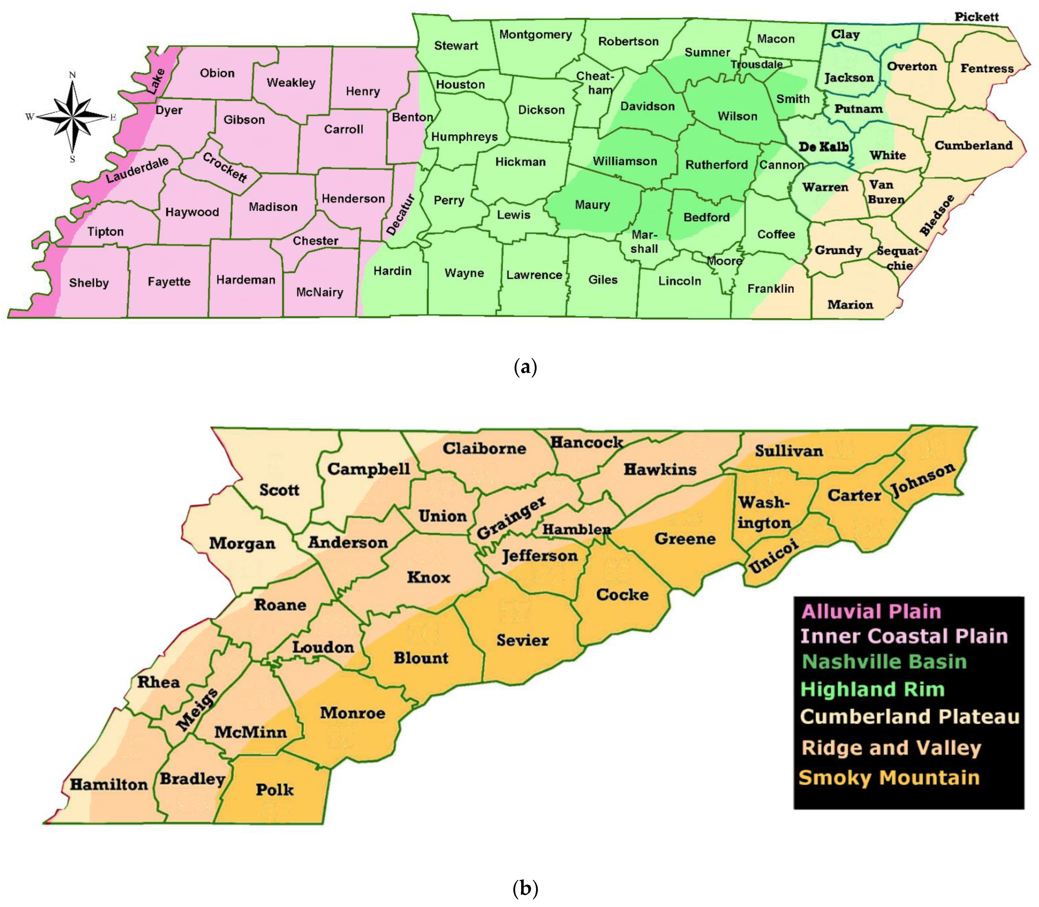
The study area is the state of Tennessee, USA, and all three types of PWSs (i.e., CWSs, NTNCs, and TNCs) are included (Figure 1). In Tennessee, there are 460 CWS, 290 TNCs, and 30 NTNCs active systems serving 7.2 million people (as of Q1 2019). We used three types of data (1) the violation data downloaded from the USEPA’s SDWIS database (2011–2018), (2) the PWS sampling data for the regulated contaminants were provided by the Tennessee Department of Environment and Conservation on April 15, 2019; and (3) the most recent income and income inequality data sets (i.e., CHR & R 2017 income and FRED 2018 income inequality) available at the county level obtained from publicly available databases [11,12].
We used the five different violation categories reported in the SDWIS database: Maximum Concentration Level (MCL), Treatment Technique (TT), Monitoring (MON), Reporting (RPT), Public Notice (PN), and Other violations. There were no reported MRDL violations during the study period. All states granted primacy must adopt federal national primary drinking water regulations standards (NPDWR) set forth by the SDWA and have the option to require stricter standards. For example, California imposes a more stringent MCL on certain contaminants, such as benzene [14].
In terms of the routine of water quality monitoring, here we have outlined the Tennessee protocol, with help from technical water experts from the state of Tennessee. PWSs are required a specific number of samples across the sampling points periodically determined by the monitoring schedule from the state primacy agency, TDEC. The samples are sent to certified laboratories for testing and measurement specific to the contaminants. TDEC indicates that it is more common for the larger PWSs to test their samples (usually biological contaminants such as total coliforms) in their own in-house certified laboratories, whereas smaller PWSs typically send their samples to the state-certified commercial laboratories. The laboratories send the results to TDEC. Next, TDEC determines if a violation has occurred and what type of violation is based on the NPDWR or if a more stringent state-level regulation is enforceable. Finally, TDEC uploads any reportable violations to the SDWIS database. MCL violation occurs if the average concentration of all the required samples exceeds the MCL of the contaminant. TT violation occurs when a treatment plant fails to comply with the requirements in the removal of specific contaminants (e.g., turbidity) or a system fails to perform a procedural requirement such as follow-up sampling for E.coli after a total coliform positive sample. Reporting of MON and RPT is more complicated. MON and RPT have two distinctions in severity, major or minor. A major MON or RPT violation is classified as a complete failure to monitor or report, whereas a minor one may be caused by providing fewer than the required number of samples, missing the reporting deadline, or not meeting the requirement. Although all monitoring and reporting violations are recorded in the SDWIS database, the annual compliance report only includes major MON/RPT violations [15]. Our research does not distinguish between major and minor MON/RPT violations.
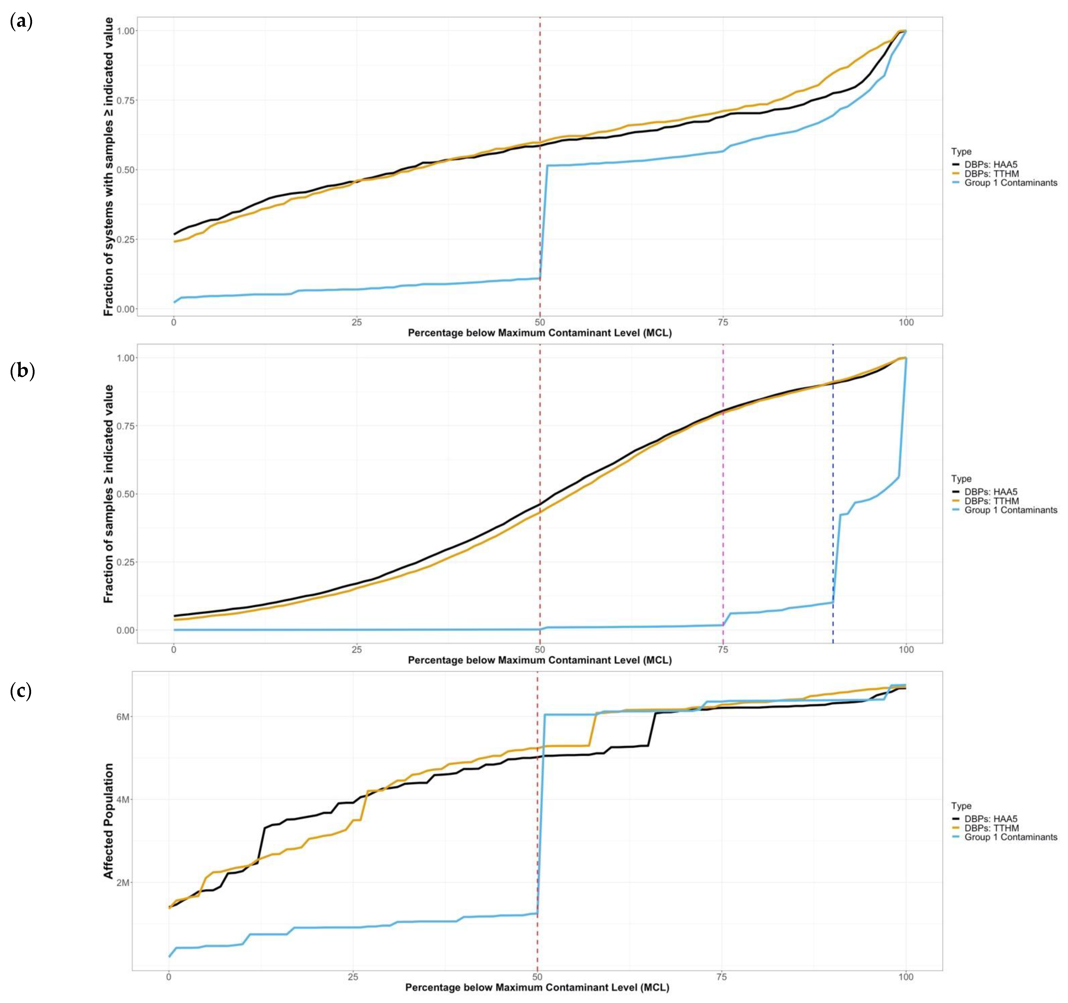
The sampling data for TN includes the raw measurements of inorganic contaminants (IOCs), synthetic organic and volatile organic contaminants (SOCs and VOCs), radionuclides (RADs), and disinfectant byproducts (DBPs). The sampling data of DBPs was stored in a separate file because DBPs have distinctly different measuring and monitoring methods. The monitoring schedule (i.e., sampling frequency and calendar time) and the number of samples for DBPs can vary by PWS based on system characteristics and monitoring framework (a monitoring framework is determined based on the size of the system and the waivers-specific systems applied for). DBPs data availability was 2012–2018, which covered as many as 678/780 systems and 6.7 million people). The two specific DBPs of chlorine disinfection, total trihalomethanes (TTHM) and haloacetic acids (HAA5), are included in the sampling data for DBPs. Therefore, we consider the IOCs, SOCs, VOCs, and RADs as group 1 contaminants, while the two DBPs are in group 2. We do not have the actual measurement of total coliforms and E. coli; therefore, these contaminants are excluded from the concentration analysis (research question 3).
We collected the latest income and income inequality data at the county level [11,12] to represent the socioeconomic capacity of the people served by a PWS. We chose the median household income as well as the income inequality, which is calculated by the top 20th percentile of the income of the earners divided by the value at the bottom 20th percentile for each of the 95 counties in Tennessee [11,12]. We used the county-level data on income and income inequality to approximate the socioeconomic conditions of the people served by the PWSs collectively in that county [16].

2.2. Categorization

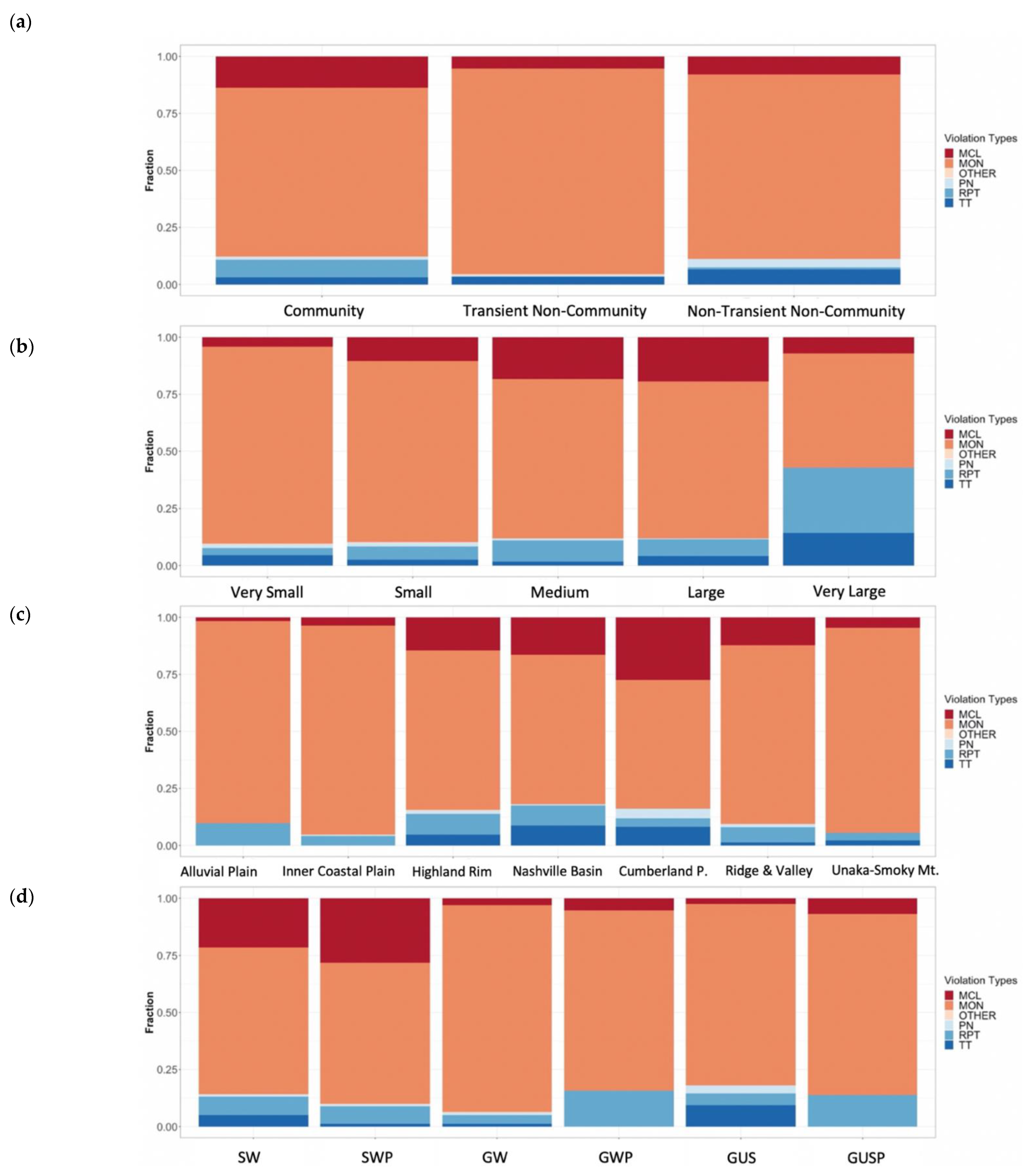
We examined the composition of the six types of SDWIS violations, MCL, TT, MON, REP, PN, and Other, by categorizing the PWSs in four different ways: types of systems, geological regions, system sizes, and types of water sources. First, there are 460 CWSs, 290 TNCs, and 30 NTNCs. Second, we categorized each PWS by matching the primary county they serve with one of the seven geological regions in Tennessee. Table 1 and Figure 1 illustrate PWS characteristics and corresponding geological regions.

2.3. MCL Levels

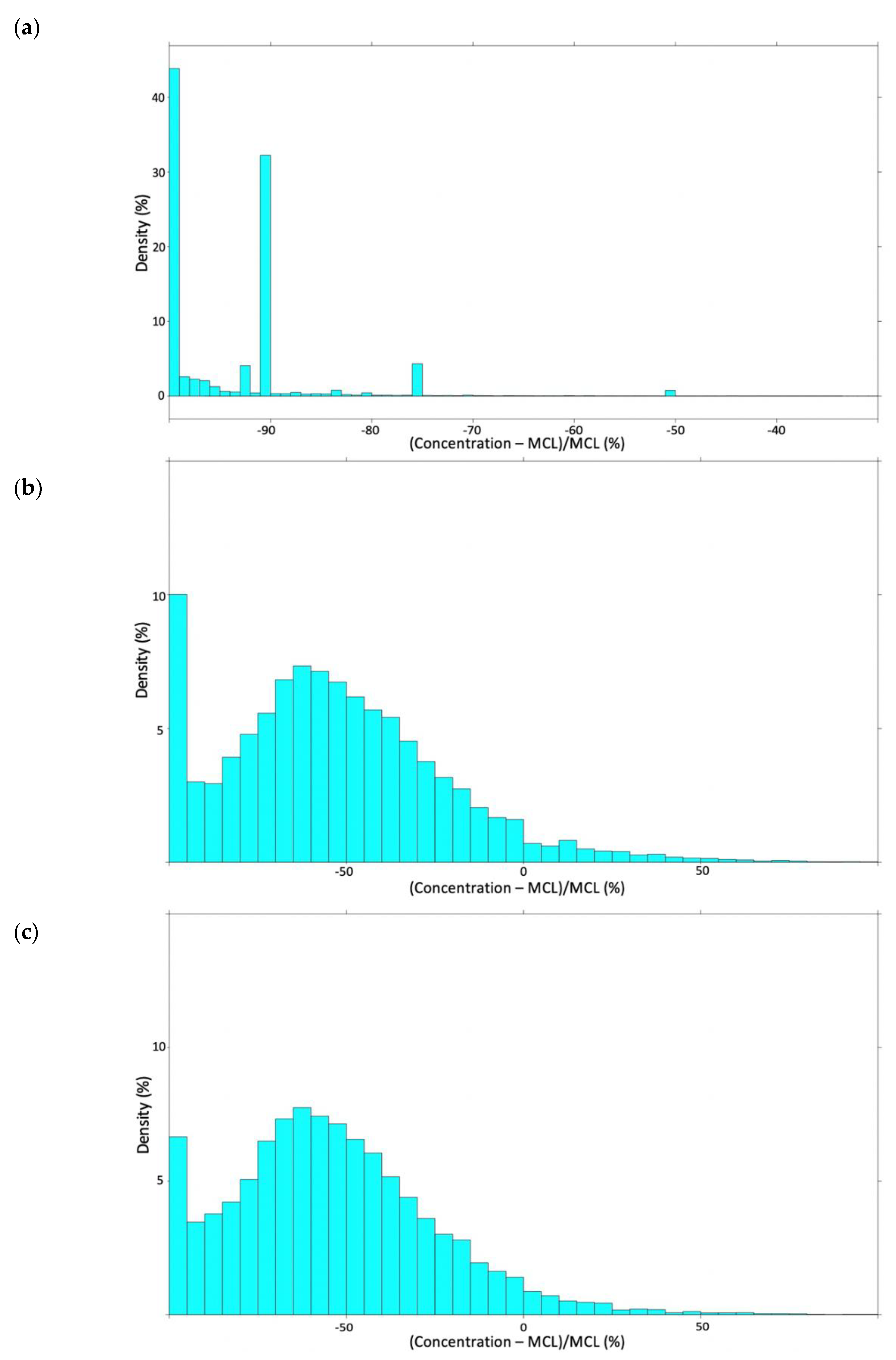
To assess the level of concentration reported in the sampling database by contaminants and compare it to the MCL, we calculated the percentage difference of each sample (PCT_DIFF_MCL) to the MCL of that specific contaminant using Equation (1). The concentrations below MCL were therefore presented as a negative percentage, the ones above MCL were shown as a positive percentage, and the MCL is at the 0 mark.
PCT _ DIFF _ MCL = C o n c e n t r a t i o n M C L M C L
We assessed the MCL levels of the IOCs, RADs, VOCs, and SOCs aggregately and individually. DBPs were analyzed separately because DBPs are formed as a result of the water treatment process and potential reaction with bromide and natural organic matter that could be present in the source water [13].
In addition to examining the concentration distributions of the aforementioned contaminants, we examined the cumulative distributions of the fraction of samples greater than or equal to the indicated value- the sample concentrations at a certain percentage point below the MCL. Similarly, we also examined cumulative distributions of the fraction of systems with samples greater than or equal to the indicated value and the affected population associated with the systems. The affected population is defined as the number of people whose water systems have samples’ concentrations greater than or equal to the indicated values.

2.4. Statistical Methods

We compared the types of violations in different categories by examining the ratio of each type of violation (MCL, MON, RPT, PN, TT, and Other) to the total number of violations. For example, among all violations of CWSs, the fraction of MCL violations is about 0.13, whereas the fraction of MCL violations among all TNC violations is only about half as much (~0.07).
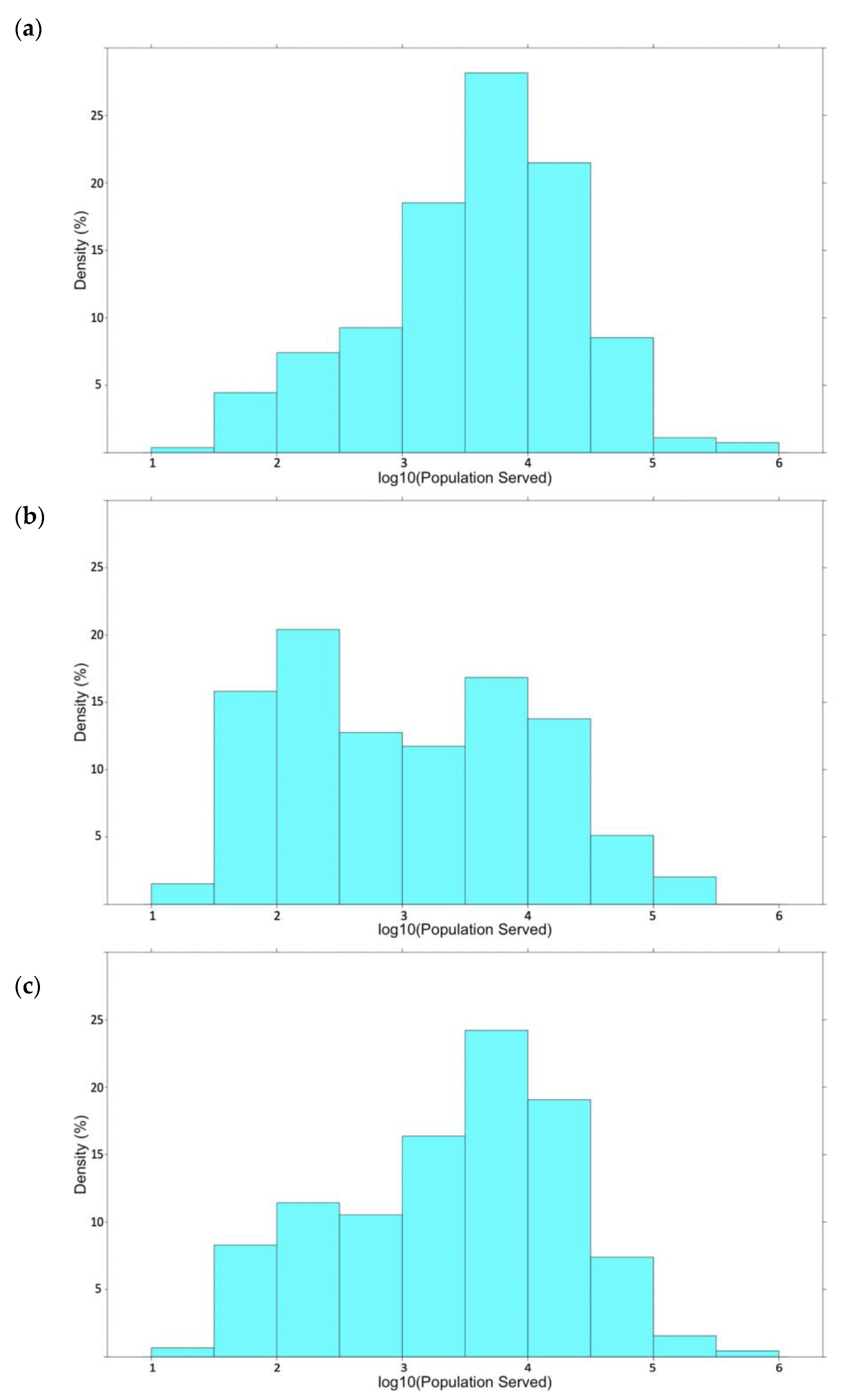
We examined the population distribution of different groups of PWSs (group 1 vs. group 2 contaminants and systems with punctuated changes at 50% of the MCL vs. systems without punctuated changes at 50% of the MCL) using Pearson’s chi-square test. We used the same bin size for the two sets of data for comparison. Because there were some bins (at the interval of 20,000 people) in the population distribution of the PWSs had counts of zero, and the population distribution was not smooth, we took the log10 transformation of the population and resampled the log10 values from 1 to 6 at the interval of 0.5. Then, we use the counts of the log10 values to perform the two-sample Pearson’s chi-square test.
We analyzed the correlation between different violation categories and income/income inequality at the county level. We use Spearman’s rank correlation coefficient to measure the relationship between two variables.

2.5. Statistical Analysis

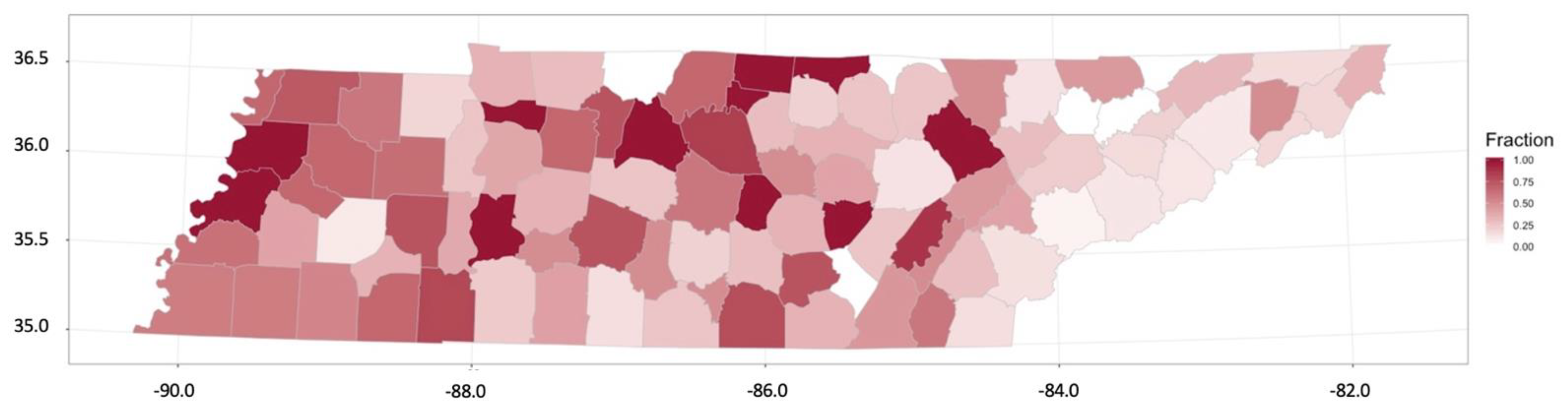
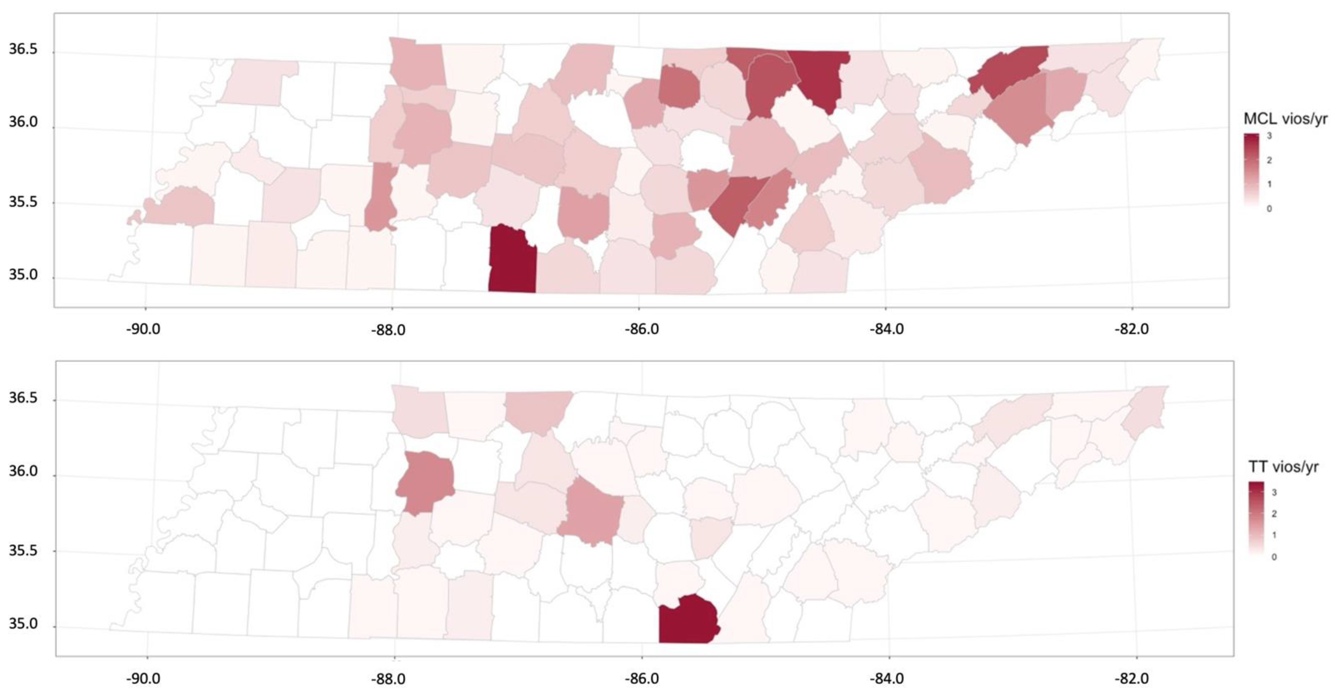
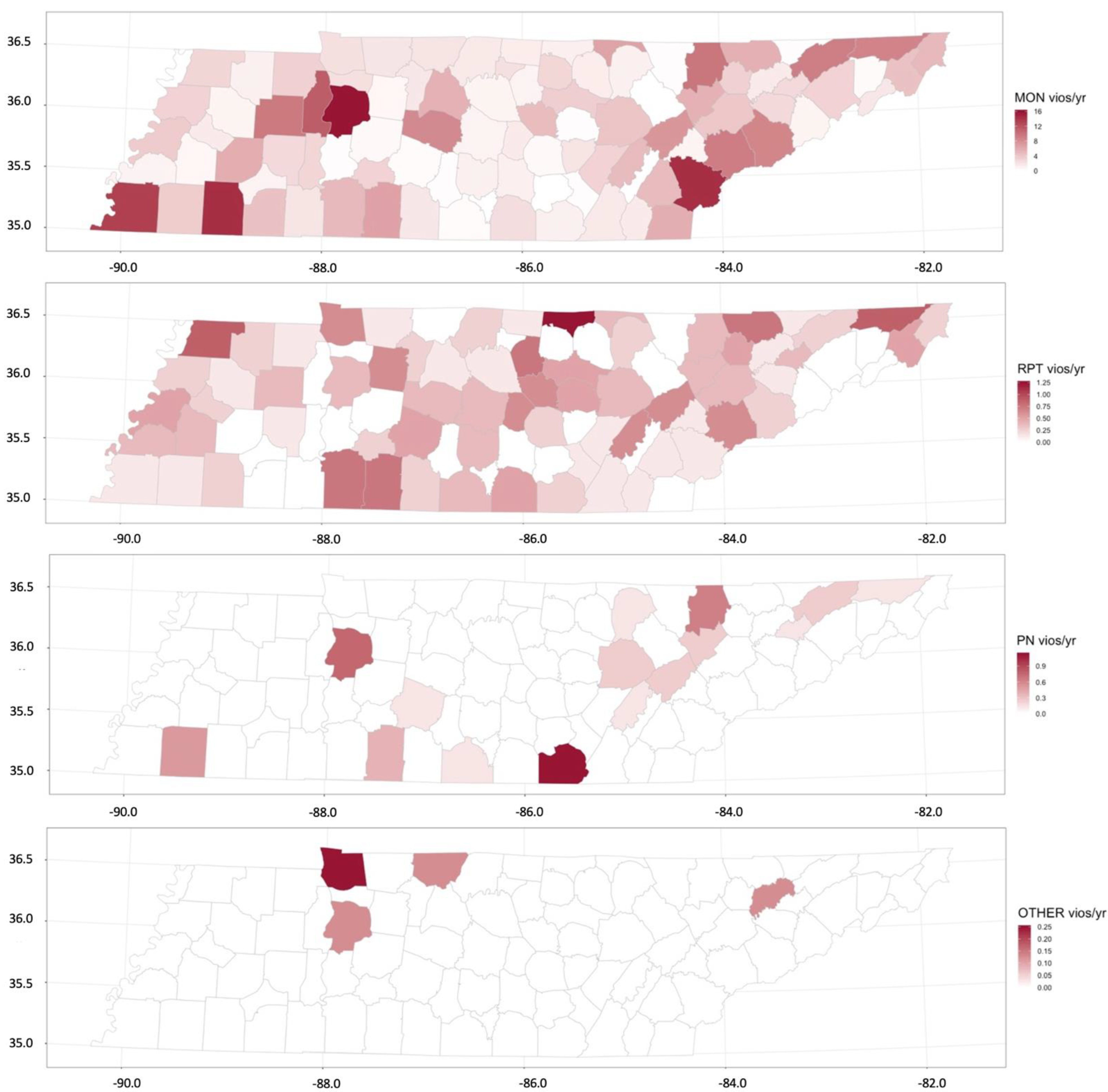
We obtained drinking water violations per year (overall and by type), median household income and income inequality, violation frequency, and long-term affected violation at the county level, and performed the Spearman rank correlation analysis. We aggregated the PWSs at the county level to report different types of violations per year by total, MON, TT, MON, RPT, PN, and Other. Those violation results of all PWSs serving the same primary county were averaged and reported for each of the 95 counties in Tennessee. In addition, we calculated two indices to reflect the violation conditions at the county level: (1) violation frequency and (2) long-term affected population. We use violation frequency as a measure of repeating violations of a system. The violation frequency (Freqviolation) is calculated using Equation (2):
F r e q v i o l a t i o n = #   y e a r s   a   s y s t e m   h a s   a n y   v i o l a t i o n t o t a l   #   o f   y e a r s
The violation frequencies of all PWSs serving the same primary county were then averaged to create a mean violation frequency for the particular county. The long-term (L.T.) affected population was created to measure the long-term impact of the violations on the people who use the water supplied by the PWSs, which is summarized at the county level. The long-term affected population is calculated using Equation (3):
L . T .   a f f e c t e d   p o p u l a t i o n = i = 1 n p o p u l a t i o n   s e r v e d v i o l a t i o n   f r e q u e n c y
where n is the total number of PWSs in the county.

2.6. Spatial Analysis

We calculated the Global Moran’s I index for each of the variables for 95 counties, which is an index used to measure the spatial autocorrelation ranging from −1 to 1 [17]. Moran’s I near 1 indicates a spatial clustering pattern (i.e., positive spatial autocorrelation), −1 indicates dissimilar dispersion (i.e., negative spatial autocorrelation), and a zero value indicates complete spatial randomness.

3. Results

3.1. Links between System Characteristics and Types of Violations

In the state of Tennessee, we found that the general violation pattern is the dominant prevalence of MON violations regardless of the categories of the PWSs (Figure 2), while other types of violations vary across the four categories: system types, system sizes, physiographic and geological factors, and water sources. Among the two types of health-based violations, the fractions of TT violations are less than the MCL violations except in the very large (VL) PWSs and PWSs using groundwater under the influence of surface water.
The CWSs have the largest fraction of MCL violations, while the TNCs have the largest MON violations. The CWSs also have significantly larger fractions of RPT and PN violations compared to the other two types of systems, TNCs and NTNCs (Figure 2).
Physiographic and geological factors are related to natural water quality and may be more correlated with MCL violations. PWSs in Cumberland Plateau (CP) have the largest fraction of the MCL violations, while PWSs in Alluvial Plain (AP) have the smallest fraction of MCL and no TT violations. For the TT violations, PWSs in the Nashville Basin (NB) and CP have the largest fractions compared to other geological regions. MCL and TT violations of PWSs in CP, NB, and Highland Rim (HR) are the top three regions that have the largest fraction of MCL and TT violations combined together. The regions toward the east and west borders of Tennessee have fewer MCL and TT violations and more MON violations than other regions (Figure 2).
MCL violations are most prevalent among medium (M) and large (L) PWSs. While other sizes of PWSs have similar fractions of MON violations, the VL PWSs only have half of the proportion. In addition, the fraction of RPT violations in VL PWSs are about three times more than the fractions of other sizes of PWSs (Figure 2).
PWSs using purchased water sources have more MCL violations and fewer TT violations compared to PWSs using non-purchased water sources. PWSs using surface water have larger fractions of MCL and TT violations compared to PWSs using groundwater. On the other hand, PWSs using groundwater sources have larger fractions of MON violations than PWSs using surface water (Figure 2).
Cumberland Plateau has the largest share of health-based violations. The medium and large systems have the largest fractions of health-based violations. The distribution of types of violations is not significantly different among Community, Transient non-community, and Non-transient non-community water systems.

3.2. Distributions of Sample Concentrations

We examined the concentration distributions of group 1 and group 2 contaminants. Most of the group 1 contaminants are below the MCL. However, there are sharp spikes in the concentration distribution, with many concentrations reported exactly at 50%, 25%, and 10% of the MCL level (Figure 3). The DBPs have a small fraction of the samples reported above the MCL, but the concentrations are mostly below 150% of the MCL level (Figure 3).
We examined the cumulative distributions of the sampling concentrations with respect to the MCL for group 1 contaminants (IOC, VOC, SOCs) and group 2 contaminants (HAA5 and TTHM). Our hypothesis was that the expected cumulative distribution of sample concentrations would be smooth and without sharp punctuated increases.
For the group 1 contaminants, a punctuated change of fractions of systems with samples greater than or equal to the indicated value occurred at 50% to 51% below MCL (Figure 4). The fraction of systems with samples greater than or equal to the indicated value of 50% below MCL was about 0.1, but as the indicated value moves 1 percent lower, the fraction increases drastically to more than 0.5. For the group 2 contaminants (DBPs), the curves were much smoother compared to the group 1 contaminants, and no punctuated changes were observed. The individual trends of the two DBPs were similar.
For the group 1 contaminants, multiple punctuated changes were observed at 50%, 75%, and 90% below MCL (Figure 4). Furthermore, the concentration distribution of the group1 contaminants indicates that there are sharp spikes on the histograms of sampling results reported exactly at 50%, 25%, and 10% of the MCL level (Figure 3), corresponding to the punctuated changes in Figure 4. A sharp spike is defined as an abnormally large number of samples reported at the same percentage. We assessed the individual concentration distribution of all the contaminants from the sampling data and found there were a large number of VOCs and some IOCs, including arsenic, cadmium, chromium, and mercury, all displaying sharp spikes at the 10% MCL level and beryllium, vinyl chloride displaying a sharp spike at the 25% MCL level, and thallium displaying a spike at the 50% MCL level (see Supplementary Materials Table S1). The concentration distributions of the individual contaminants are included in the Supplementary Materials (see Supplementary Figures S1–S4).
For the DBPs, the fraction of samples greater than or equal to indicated values exhibited a similar smooth increasing trend as concentrations decreased below the MCL level (Figure 4). The shape of the concentration distributions of HAA5 and TTHM appears similar, but they are not from the same distribution (p < 2.2 × 10⁻¹⁶ from Pearson’s chi-square two-sample test, Figure 3).
For the group 1 contaminants, there were multiple-step increases, and a punctuated change in population occurred at 50–51% below the MCL level (Figure 4). Compared to the previous changes in the number of violations and number of systems having violations, the punctuated change in population at 50–51% MCL was disproportionally large. The punctuated change of the affected population (close to 4 million population increase) indicated that it was not solely driven by the large systems. From the population distribution of the PWSs that demonstrated a punctuated change, the M and L PWSs were dominant (Figure 5). All the VL systems that serve more than 300,000 people were included in the punctuated change. We compared the population distribution of the systems that displayed the punctuated change with systems that did not display such change to the overall population and found the distribution of the systems with punctuated changes is more similar to the overall population distribution (p = 0.37 from chi-square two-sample test, Figure 5). Geographically, the systems that displayed punctuated change are concentrated at AP and the northern part of HR and NB (Figure 6).
For the DBPs, the affected population went up with several step changes as concentrations reduced from 100% to 0% of the MCL, and the two largest step changes occurred at different levels for TTHM (57%) and HAA5 (66%) (Figure 4). However, the magnitudes of the step changes are identical, which indicates that the changes are driven by the largest two systems serving major cities (Nashville and Memphis, which each serve 700 thousand people).
Neither the median household income nor income inequality showed a strong association with total, MCL, or monitoring violations at the county level. However, there were weak positive associations observed between income and reporting, public notice, other, and TT violations. A weak negative association was observed between income inequality and reporting, public notice, other, and TT violations (Table 2) (The complete correlation coefficient matrix with the distribution of the data is in supplementary information). In addition, income inequality was weakly associated with the fraction of the systems that demonstrated punctuated change among all systems in the counties. Therefore we did not find strong evidence indicating a clear relationship between income and income inequality and drinking water violations. However, future research at the scale of the service area of PWSs could better capture the sub-county socioeconomic nuances and differences such as segregation and gentrification when relevant data are available.

3.3. Spatial Patterns of Drinking Water Quality

From the Moran’s I indices, only the systems that demonstrated punctuated change (Figure 6) and MCL violations (Figure 7) showed slight clustering patterns. Although we found little evidence of spatial clustering, there were several counties in each of the maps that revealed higher values than their neighbors (Table 3, and Figure 6, Figure 7 and Figure 8). Specifically, most of the violations are monitoring violations of inorganic, organic, and microbial contaminants in Humphreys County. DBPs are the most frequent contaminant of the MCL violations in Giles County. TT violations of combined filter effluent and PN violations about notifying the public about violations are most prevalent in the systems of Marion County. RPT violations of record-keeping are most prevalent in Clay County. The only Other violations of siting plan errors are most prevalent in Stewart County. Pickett, Trousdale, Cannon, and Van Buren counties have significantly higher values of violation frequency than other counties (Figure 1). Shelby County has the highest value of long-term affected population among all counties, where 106 of 107 records of violations are monitoring violations of different contaminants, and one is a reporting violation (Figure 1).

4. Discussion

How do system size and type influence drinking water violations? We first found that very small (VS) and small (S) PWSs predominantly have smaller fractions of MCL violations and a larger proportion of MON violations compared to larger PWSs (medium M and Large L); the exception is 9 (represents approximately 1.2% of total PWSs in TN) of the very large (VL) PWSs. The finding is consistent with TNCs and NTNCs as they also have much smaller fractions of MCL violations compared to CWSs because most of TNCs and NTNCs are very small (VS) and small (S) PWSs, which is similar to the conditions in Virginia [6]. However, such a finding is contradictory to a prior study that found fewer MCL violations in larger PWSs [5]. The smaller fractions of MCL violations found in smaller systems are also contradictory to one of the findings in a national-level analysis [1]. One possible reason to explain the finding is that the larger PWSs have a greater capacity to test the water and report the result on time (in-house laboratory). Therefore, larger PWSs may have a larger fraction of MCL violations, whereas smaller PWSs may be more prone to MON violations due to stressed technical, managerial, and financial capacity (e.g., additional time required to submit samples to an external laboratory for testing) [18]. The EPA monitoring framework and other specific rules of TDEC require large numbers of samples to be tested in a relatively short time period (such as DBPs) [19]. Larger PWSs equipped with in-house (or on-site) laboratories can handle the load of testing more efficiently. Smaller systems may encounter human errors due to a lack of organizational and management skills and forget to submit samples, which could explain the larger fractions of MON violations in smaller PWSs.
How does source water influence drinking water violations? We found that the PWSs using groundwater are associated with smaller fractions of MCL violations in Tennessee. A potential reason is that the raw groundwater may be cleaner as the physical, chemical, and biological contaminants are gradually removed when the groundwater flows through the vadose zone and the aquifer [20]. In addition, PWSs using groundwater also need to treat the water to comply with the regulations. PWSs from Alluvial Plain, Ridge and Valley, and Unaka-Smokey Mountain that source water from deep-underground aquifers, such as the Memphis Sand and the East Tennessee Aquifer, have the lowest fractions of MCL violations in Tennessee [21,22]. It is worth noting that the groundwater-sourced systems are not required to test their water as frequently as the surface-sourced systems for certain contaminants. Yet, it is unclear if the low frequency of MCL violations is related to the less frequent monitoring frequency.
In addition to groundwater vs. surface water, PWSs using purchased water experience higher fractions of MCL violations in Tennessee, which is contradictory to the results of national-level research [1]. Allaire et al. [1] attribute the lower MCL violations of PWSs using purchased water to the purchased source being private wholesalers (1) with a high capacity to comply with drinking water standards and (2) who are more vulnerable to lawsuits if supplied drinking water does not meet regulatory standards. In Tennessee, the majority of the PWSs, including wholesalers, are public-owned, so such an explanation may not be applicable. One potential reason is that the purchased water is subject to contamination through the distribution network or during storage. For instance, the common practice for ensuring drinking water quality through distribution is to keep the disinfectant (typically residual chlorine) at a certain level that can keep the water sanitized but not harmful for human consumption. DBPs are formed when organic matter reacts with chlorine. The DBP-forming process can be affected by various factors such as the specific chemicals and the doses for disinfection, the concentration of the precursors that react with the chemical, the pH, temperature, and water age [23]. Another reason pointed out by an EPA study is that the system’s water received from the wholesaler at the interconnection may continue to rise in DBP concentration level as the disinfectants keep reacting during the distribution process [23].
How do physiographic and geological factors influence drinking water violations? We found that PWSs in Nashville Basin (NB) and Cumberland Plateau (CP) have much higher fractions of MCL violations compared to other regions. The potential reason could be the relatively high concentrations of contaminants such as regulated IOCs that are naturally present on the topsoil layers (~1 m) in Tennessee, particularly concentrated in HR, NB, and CP [24]. In Tennessee, the concentrations of antimony, arsenic, beryllium, cadmium, total carbon, organic carbon, chromium, mercury, and thallium generally are higher than the national average, and the highest concentrations of the listed contaminants are concentrated in northeast HR, the north NB, and northwest CP (hereafter the first concentrated region), and the Alluvial Plain (hereafter the second concentrated region) (Figure 7; [24].
How does where people live influence water quality? An interesting finding of our research is that many of the PWSs that displayed punctuated change in reported concentrations of the contaminants exactly at the 50% MCL level are located within the two aforementioned concentrated regions (Figure 6). It is less likely that the systems have the technical sophistication to intentionally treat the water just under 50% of the threshold. Therefore, some punctuated change at 50% may be coincidental. However, future studies could investigate those water samples at just below 50% MCL in detail to figure out the causes for such a large number of samples reported at the same percentage level.
It is also noticeable to see that the first concentrated region has the highest fractions of MCL violations, whereas the second concentrated region has the lowest. One probable reason is that most of the PWSs in the first concentrated regions are using surface water, whereas all PWSs in the second concentrated region (AP) are sourcing groundwater, and groundwater sources have better quality, as noted above.
The counties with the highest values varied spatially in Tennessee; however, there are some commonalities among them (Figure 1, Figure 6, Figure 7 and Figure 8. All four counties, Pickett, Trousdale, Cannon, and Van Buren, had the highest violation frequencies and used surface water where large river bodies (i.e., the Cumberland River, and large reservoirs with hydropower generation capacity, including Dale Hollow Lake, Cordell Hull Lake, and Center Hill Lake) run through or nearby their land. Large impoundments of water create issues that impact water quality, such as eutrophication, low dissolved oxygen due to the photosynthesis of excess algae, etc. While we do not know the source water quality at times when monitoring violations of various inorganics and organic contaminants occurred, most of the MCL violations were DBPs (Supplemental Information), so it may be that source waters were high in dissolved organic carbon at these times. Another probable cause could be the systems’ failure to remove the contaminant during the treatment process adequately and failure to manage the distribution residence time. A few water systems had a treatment technique violation due to a lack of qualified water system operators.
Excessive numbers and frequency of monitoring and reporting violations of all types of public water systems are of concern. Much previous research has focused on the MCL and TT violations because these are explicitly associated with health risks. However, if a system fails to report a contaminant measure, the resulting major or minor monitoring reporting violation could simply mask a problem. At the time of a monitoring violation, neither the authorities nor consumers should have confidence that the drinking water is safe. The uncertainties associated with monitoring violations require attention in the current public water systems operations as well as SDWA oversight and enforcement.
How close are the sample measurements to the MCL? The majority of the samples are below the MCL. Most of the samples in violation are below 150% of MCL. However, we saw spikes at 10%, 25%, and 50% of the MCL level for group 1 contaminants. The concentration distributions indicated that large numbers of samples are reported exactly at these three percentages. This may not be a significant issue since the concentrations are still relatively low. Nevertheless, higher concentrations of contaminants, even under the MCL, may be harmful to certain vulnerable groups of people who are more sensitive than an average person, such as pregnant women, persons with diabetes, and children under 5 years old.

Strengths/Limitations

The article used both the SDWIS violation data as well as the sampling data to examine the potential contributing factors to drinking water quality in the state of Tennessee. However, due to limited data availability, the findings may not be applicable to other states. Another limitation is that the research is conducted at the county level rather than the PWS level. Aggregating data to higher spatial level is not ideal because some finer level dataset were not used to its full potential, but it is not uncommon in spatial data analyses [25]. Aggregating to county allows for comparison of our results to other studies as the vast majority aggregate to the county. Yet, the aggregation of all violation data from multiple PWSs to a county may result in loss of information, so researchers cannot investigate critical issues such as the drinking water quality in underrepresented groups.

5. Conclusions

In this study, we used both the sampling data of contaminants in PWSs as well as the SDWIS violation records to study the factors that influence the drinking water quality of PWSs in Tennessee. We find that different types of violations are related to geological factors, population density, and water source. We also find that the distribution of measured concentrations for many contaminants is punctuated by discontinuities at selected levels, such as at 50% of the MCL specified in EPA regulations.
The current study demonstrates the importance of using both sampling and SDWIS data to study the drinking water quality and reveal more nuances of drinking water violations. Our data analysis strategy revealed anomalous spikes in the cumulative distribution of measured concentrations at 10%, 25%, and 50% of the MCL level for group 1 contaminants. These anomalous spikes are of concern because contaminant concentrations below the MCL carry no imprimatur of absolute safety. There is a growing concern about the relationship between contaminant concentrations below the MCL in drinking water and health [26]. The issue of water samples at just below 50% MCL is an intriguing one, which could be usefully explored in further research to identify contributing factors, such as measurement protocol and equipment, and environmental and social factors (i.e., geological or population density). Additional research studies are needed at a more granular level (i.e., the PWS level) using sampling data to understand better the impacts of drinking water violations and the full range of measured concentrations on different communities. A recommended policy action is a nationwide geospatial database that stores the geographic information of PWSs, drinking water quality (i.e., SDWIS and sampling), and other environmental and socioeconomic data that could significantly advance drinking water research in the US [27].

Supplementary Materials

The following supporting information can be downloaded at: https://www.mdpi.com/article/10.3390/w14162562/s1, Figure S1: Individual concentration distributions of inorganic contaminants (IOC). Red dashed line in each subplot indicates the Maximum Contamination Level (0% difference from MCL); Figure S2: Individual concentration distributions of radionuclides (RAD). Red dashed line in each subplot indicates the Maximum Contamination Level (0% difference from MCL); Figure S3: Individual concentration distributions of Synthetic Organic Contaminants (SOC). Red dashed line in each subplot indicates the Maximum Contamination Level (0% difference from MCL); Figure S4: Individual concentration distributions of volatile organic contaminants (VOC); Table S1: Summary of concentration distributions of IOC, RAD, SOC, and VOC.

Author Contributions

Conceptualization, K.J.D., Y.J.M., G.M.H. and E.L.H.; methodology, K.J.D., Y.J.M., G.M.H. and E.L.H.; software, K.J.D.; validation, K.J.D. and Y.J.M.; formal analysis, K.J.D.; investigation, K.J.D. and Y.J.M.; resources, Y.J.M.; data curation, Y.J.M. and K.J.D.; writing—original draft preparation, K.J.D., Y.J.M. and G.M.H.; writing—review and editing, Y.J.M., K.J.D., G.M.H. and E.L.H.; visualization, K.J.D.; supervision, Y.J.M. and G.M.H.; project administration, Y.J.M. and G.M.H.; funding acquisition, Y.J.M., G.M.H. and E.L.H. All authors have read and agreed to the published version of the manuscript.

Funding

This work is funded by Vanderbilt University Interdisciplinary Grant. Elaine L. Hill supported by NIH Award: DP5OD021338.

Institutional Review Board Statement

Not applicable as this study did not involve humans or animals.

Informed Consent Statement

Not applicable as this study did not require informed consent.

Data Availability Statement

SDWIS data is publicly available in USEPA’s database. This study used sampling data provided by the Tennessee Department of Environment and Conservation provided, which was not publicly available during the study analyses period. These sampling data of drinking water quality in Tennessee are now publicly available at https://dataviewers.tdec.tn.gov/DWW/ (accessed on 1 June 2022).

Acknowledgments

The authors would like to thank Thushara Gundafor her feedback on the conceptualization of the research design. The authors would also like to thank Judy Manners, Tennessee Department of Health and David Money, Tennessee Department of Environment and Conservation, for their expertise and feedback on the article. We also thank the Vanderbilt University Drinking Water Justice Lab for their ongoing support.

Conflicts of Interest

The authors declare no conflict of interest.

References

  1. Allaire, M.; Wu, H.; Lall, U. National trends in drinking water quality violations. Proc. Natl. Acad. Sci. USA 2018, 115, 2078–2083. [Google Scholar] [CrossRef] [PubMed] [Green Version]
  2. Rubin, S.J. Evaluating violations of drinking water regulations. J.-Am. Water Work. Assoc. 2013, 105, E137–E147. [Google Scholar] [CrossRef]
  3. McDonald, Y.J.; Jones, N.E. Drinking Water Violations and Environmental Justice in the United States, 2011–2015. Am. J. Public Health 2018, 108, 1401–1407. [Google Scholar] [CrossRef] [PubMed]
  4. Eskaf, S.; UNC Environmental Finance Center. The Environmental Finance Blog. Small Water Systems with Financial Difficulties Are More Likely to Violate EPA Regulations. 2015. Available online: http://efc.web.unc.edu/2015/01/28/small-water-systems-financial-difficulties-likely-violate-epa-regulations/ (accessed on 12 June 2019).
  5. Kirchhoff, C.J.; Flagg, J.A.; Zhuang, Y.; Utemuratov, B. Understanding and Improving Enforcement and Compliance with Drinking Water Standards. Water Resour. Manag. 2019, 33, 1647–1663. [Google Scholar] [CrossRef]
  6. Marcillo, C.E.; Krometis, L.H. Small towns, big challenges: Does rurality influence Safe Drinking Water Act compliance? AWWA Water Sci. 2019, 1, e1120. [Google Scholar] [CrossRef] [Green Version]
  7. Schaider, L.A.; Swetschinski, L.; Campbell, C.; Rudel, R.A. Environmental justice and drinking water quality: Are there socioeconomic disparities in nitrate levels in U.S. drinking water? Environ. Health 2019, 18, 3. [Google Scholar] [CrossRef] [PubMed] [Green Version]
  8. Hill, E.; Ma, L. Shale Gas Development and Drinking Water Quality. Am. Econ. Rev. 2017, 107, 522–525. [Google Scholar] [CrossRef] [PubMed] [Green Version]
  9. Hill, E.L.; Ma, L. Drinking water, fracking, and infant health. J. Health Econ. 2022, 82, 102595. [Google Scholar] [CrossRef] [PubMed]
  10. Pennino, M.; Leibowitz, S.G.; Compton, J.E.; Hill, R.A.; Sabo, R.D. Patterns and predictions of drinking water nitrate violations across the conterminous United States. Sci. Total Environ. 2020, 722, 137661. [Google Scholar] [CrossRef] [PubMed]
  11. CHR & R; University of Wisconsin Population Health Institute. Median Household Income in Tennessee. 2019. Available online: https://www.countyhealthrankings.org/app/tennessee/2019/measure/factors/63/data (accessed on 2 February 2020).
  12. FRED. 2018, Income Inequality, Annual: Tennessee. 2019. Available online: https://fred.stlouisfed.org/release/tables?rid=414&eid=303754#snid=303773 (accessed on 2 February 2020).
  13. Tennessee Department of Environment and Conservation, Air Pollution Control Division. 2022 Tennessee Annual Monitoring Network Plan 2022. Available online: https://www.tn.gov/content/dam/tn/environment/air/documents/apcairqualitymonitoring/apc_2022-tennessee-annual-monitoring-network-plan-final.pdf (accessed on 1 June 2022).
  14. California Water Boards. Contaminants in Drinking Water. 2022. Available online: https://www.waterboards.ca.gov/drinking_water/certlic/drinkingwater/Chemicalcontaminants.html (accessed on 7 January 2022).
  15. US EPA. SDWIS Overview. 2019. Available online: https://www.epa.gov/enviro/sdwis-overview (accessed on 2 February 2020).
  16. Bernabé, E.; Sheiham, A.; Sabbah, W. Income, Income Inequality, Dental Caries and Dental Care Levels: An Ecological Study in Rich Countries. Caries Res. 2009, 43, 294–301. [Google Scholar] [CrossRef] [PubMed]
  17. UCLA Institute for Digital Research and Education; IDRE. How Can I Calculate Moran’s I in R?|R FAQ. 2020. Available online: https://stats.idre.ucla.edu/r/faq/how-can-i-calculate-morans-i-in-r/ (accessed on 2 February 2020).
  18. Balazs, C.L.; Morello-Frosch, R. The Three Rs: How Community-Based Participatory Research Strengthens the Rigor, Relevance, and Reach of Science. Environ. Justice 2013, 6, 9–16. [Google Scholar] [CrossRef] [PubMed] [Green Version]
  19. US EPA. The Standardized Monitoring Framework: A Quick Reference Guide, Water; US EPA: Washington, DC, USA, 2004.
  20. Moore, J.E. Groundwater Quality; Wiley & Sons: New York, NY, USA, 2005; pp. 406–407. [Google Scholar] [CrossRef]
  21. Brahana, J.V.; Mulderink, D.; Macy, J.A.; Bradley, M.W. Preliminary Delineation and Description of the Regional Aquifers of Tennessee—The East Tennessee Aquifer System; Water-Resources Investigations Report 82-4091; US Department of the Interior: Washington, DC, USA, 1986.
  22. Parks, W.S.; Carmichael, J.K. Geology and Ground-Water Sources of the Memphis Sand in Western Tennessee; US Department of the Interior: Washington, DC, USA, 1990.
  23. US EPA. Stage 2 Disinfectants and Disinfection Byproducts Rule (DBPR) and Consecutive System In-Depth Analysis 35; US EPA: Washington, DC, USA, 2019.
  24. Smith, D.; Cannon, W.F.; Woodruff, L.G.; Solano, F.; Ellefsen, K.J. Geochemical and Mineralogical Maps for Soils of the Conterminous United States; USGS: Reston, VA, USA, 2014. [CrossRef]
  25. Ding, K.J.; Gunda, T.; George, M.H.; Hornberger, G.M. Prominent Influence of Socioeconomic and Governance Factors on the Food-Energy-Water Nexus in sub-Saharan Africa. Earth’s Future 2019, 7, 1071–1087. [Google Scholar] [CrossRef] [Green Version]
  26. DiSalvo, R.; Hill, E.L. The effects of drinking water contamination on birth outcomes: New estimates from drinking water samples. Working Paper.
  27. McDonald, Y.J.; Anderson, K.M.; Caballero, M.D.; Ding, K.J.; Fisher, D.H.; Morkel, C.P.; Hill, E.L. A systematic review of geospatial representation of United States community water systems. AWWA Water Sci. 2022, 4, e1266. [Google Scholar] [CrossRef]
Figure 1. The 95 counties in the state of Tennessee and their geological regions by (a) Central Time Zone Regions (CST UTC-6:00, CDT UTC-5:00) and (b) Eastern Time Zone Regions (CST UTC-5:00, CDT UTC-4:00) [13].
Water 14 02562 g001
Figure 2. Fractions of the types of violations by (a) types of the water systems, (b) sizes of the systems, (c) geological regions, and (d) sources of water. Purchased water, in general, has a higher share of MCL-based violations and fewer TT violations in comparison to systems that treat their own water.
Water 14 02562 g002
Figure 3. Sampling concentration distributions of (a) Group 1 contaminants (inorganics/organics), (b) haloacetic Acids (HAA5), and (c) total trihalomethane (TTHM), from top to bottom, respectively.
Water 14 02562 g003
Figure 4. Cumulative distributions of (a) fractions of systems with samples greater or equal to indicated value concentration below percentages of MCL, (b) fractions of samples greater or equal to indicated value, (c) and affected population for group 1 contaminants of Inorganic, organic, and radionuclides (cyan), TTHM (gold), and HAA5 (black). The punctuated changes at 50%, 75%, and 90% of the MCL are indicated by the vertical dash lines in red, magenta, and blue, respectively.
Water 14 02562 g004
Figure 5. log10 (population) distributions of (a) the systems having punctuated changes when MCL lowered from 50% to 49%; (b) the complement of systems in part 1 (systems did not have punctuated changes); (c) all systems.
Water 14 02562 g005
Figure 6. Spatial distribution of the systems with punctuated changes. Note: Intensity of the color represents the fraction: #   of   systems   with   punctuated   changes #   of   systems   in   the   same   county . The MCL maps shows slight spatial clustering patterns (Moran’s I = 0.126, p-value = 0). The x axis is longitude, the y axis is latitude.
Water 14 02562 g006
Figure 7. Maps of maximum contaminant level (MCL) violations and Treatment Technique (TT) violations per county per year. Note: MCL and TT violations are health-based violations according to the EPA definition. The MCL maps shows slight spatial clustering patterns (Moran’s I = 0.022, p-value = 0.02). The x axis is longitude, the y axis is latitude.
Water 14 02562 g007
Figure 8. Maps of monitoring (MON) violations, reporting (RPT) violations, Public Notice (PN) violations, and other (OTHER) violations per county per year. The x axis is longitude, the y axis is latitude.
Water 14 02562 g008
Table 1. Public Water System Characteristics and Geological Region.
PWS TypeNumber of of SystemsGeological RegionNumber of SystemsSystem Size by Population ServedNumber of SystemsWater SourcesNumber of Systems
CWS460AP15VS (0–300)348SW151
TNC290ICP175S (301–3300)163SWP120
NTNC30HR178M (3301–10,000)132GW432
NB44L (10,001–100,000)128GWP13
CP52VL (>100,001)9GUS55
RV165 GUSP9
USM151
Note: PWS represents public water system; CWS represents community water system; TNC represents transient non-community water system; NTNC represents non-transient non-community water system; AP represents Alluvial Plain; ICP represents Inner Coastal Plain; HR represents Highland Rim; NB represents Nashville Basin; CP represents Cumberland Plateau; RV represents Ridge and Valley, and USM represents Unaka-Smoky Mountain; VS, S, M, L, and VL represent very small, small, medium, large, and very large public water systems, respectively; SW, SWP, GW, GWP, GUS, and GUSP represent public water systems sourced from surface water, surface water purchased, groundwater, groundwater purchased, groundwater under the influence of surface water, and groundwater under the influence of surface water purchased, respectively.
Table 2. Spearman’s rank correlation coefficients matrix.
TotalMCLMONRPTPNOtherTTFractionVio Freq
Income−0.00058−0.05030.01210.1240.1330.1410.1250.0643−0.0681
Income Inequality−0.0197−0.027−0.003760.06090.033−0.234−0.1810.1460.0704
Table 3. Counties with the highest values of different types of violations and indices.
Metrics/IndicesCounties with Highest ValuesNumber of CWSsNumber of TNCsNumber of NTNCTotal Population Served
Total/MON violation per yearHumphreys43815,444
MCL violations per yearGiles60030,259
TT/PN violations per yearMarion3208648
RPT violations per yearClay2009624
OTHER violations per yearStewart6307697
Long-Term Affected ViolationShelby601939,108
Violation FrequencyPickett1007060
Trousdale1008055
Cannon10010,505
Van Buren1005217
Publisher’s Note: MDPI stays neutral with regard to jurisdictional claims in published maps and institutional affiliations.

