Article

A Comparative Evaluation of Conceptual Rainfall–Runoff Models for a Catchment in Victoria Australia Using eWater Source

by
Najibullah Zafari
1,
Ashok Sharma
1,
Dimuth Navaratna
1,
Varuni M. Jayasooriya
2,
Craig McTaggart
3 and
Shobha Muthukumaran
1,*
1
Institute for Sustainable Industries & Liveable Cities, College of Engineering and Science, Victoria University, Footscray, VIC 3011, Australia
2
Department of Forestry and Environmental Science, Faculty of Applied Sciences, University of Sri Jayewardenepura, Nugegoda 10250, Sri Lanka
3
Barwon Water, Geelong, VIC 3220, Australia
*
Author to whom correspondence should be addressed.
Water 2022, 14(16), 2523; https://doi.org/10.3390/w14162523
Submission received: 30 June 2022 / Revised: 4 August 2022 / Accepted: 6 August 2022 / Published: 16 August 2022

Abstract

:
Hydrological modelling at a catchment scale was conducted to investigate the impact of climate change and land-use change individually and in combination with the available streamflow in the Painkalac catchment using an eWater Source hydrological model. This study compares the performance of three inbuilt conceptual models within eWater Source, such as the Australian water balance model (AWBM), Sacramento and GR4J for streamflow simulation. The three-model performance was predicted by bivariate statistics (Nash–Sutcliff efficiency) and univariate (mean, standard deviation) to evaluate the efficiency of model runoff predictions. Potential evapotranspiration (PET) data, daily rainfall data and observed streamflow measured from this catchment are the major inputs to these models. These models were calibrated and validated using eight objective functions while further comparisons of these models were made using objective functions of a Nash–Sutcliffe efficiency (NSE) log daily and an NSE log daily bias penalty. The observed streamflow data were split into three sections. Two-thirds of the data were used for calibration while the remaining one-third of the data was used for validation of the model. Based on the results, it was observed that the performance of the GR4J model is more suitable for the Painkalac catchment in respect of prediction and computational efficiency compared to the Sacramento and AWBM models. Further, the impact of climate change, land-use change and combined scenarios (land-use and climate change) were evaluated using the GR4J model. The results of this study suggest that the higher climate change for the year 2065 will result in approximately 45.67% less streamflow in the reservoir. In addition, the land-use change resulted in approximately 42.26% less flow while combined land-use and higher climate change will produce 48.06% less streamflow compared to the observed flow under the existing conditions.

1. Introduction

Precise forecasts of catchment streamflow are needed to help the water authority to make a better decision on water planning and management. In Australia, the small amount of rainfall water becomes runoff and yearly variance in streamflow is greater than in other countries [1,2]. In addition to climate change, land-use change is also caused by human activity that can impact the quantity and quality of runoff [3]. Climate modelling indicates that south-east Australia will be drier in the future [4]. Hydrological models are important tools for the planning, design and management of water resource systems. Currently, several hydrological models have been greatly used for obtaining the appropriate solutions for numerous environmental problems of catchments. According to Legesse [5], hydrological models can be classified into three categories: empirical or black-box; physically-based distributed or white-box; and conceptual or grey-box models. The empirical models do not consider the governing physical laws of the process involved and only relate input to output through some transform function [6]. The distributed models have the ability to present the spatial variability of processes, boundary conditions and parameters to some degree; however, they are minimal due to the excessive need of data and computational time [7]. On the other hand, conceptual models represent the effective response of an entire catchment, without attempting to characterise the spatial variability of the response explicitly; however, they normally need fewer inputs to model streamflow in response to precipitation conceptually with acceptable accuracy [8]. Regardless of their lumped nature, these conceptual models are used in a wide range of hydrological applications, such as the estimation of catchment runoff, analysing the impact of climate and land-use change on runoff, and support water engineers and hydrologists for managing the water resources.
However, the selection of suitable models for the hydrologic assessment is one of the significant aspects of modelling practices, especially in data-sparse environments. In addition, one of the most difficult aspects of managing the water systems is bringing all of the management tools together on a single platform. Currently, single platforms such as the Source modelling platform developed by eWater limited, Australia accommodate all the details of the catchment; different rainfall–runoff models are used for hydrological studies [9,10]. Around 11 rainfall–runoff models are included in the Source framework, including three rainfall–runoff models, such as GR4J, the Australian water balance model (AWBM) and Sacramento used in this study. The selected conceptual models are commonly used in Europe, the USA and Australia to predict runoff; they can be used for land-use and climate change impact on streamflow [1,11]. These three rainfall–runoff models were selected due to being simple conceptual rainfall–runoff models [12]. GR4J and AWBM have a simple structure and faster calibration processes [13]. The AWBM model has been used to model the effect of climate change on streamflow in Australia [14]. The Sacramento model has been studied extensively and used in forecasting runoff [15]. The GR4J model has been proven to be more effective than complex models such as TOPMODEL, IHACRES, etc. [7].
Information on streamflow is a vital component of most aspects of water resource management. The enhanced streamflow forecasting capability will provide multiple benefits, including improved water-use efficacy via better anticipation of river inflows, an enhanced ability to predict the volumes and timing for flood events, and a related reduction in operational losses due to over releases from water storage [10]. Catchment characterisation, land-use and land-cover are some of the key factors affecting the performance of rainfall–runoff modelling [3]. The runoff generation process in a rural or regional catchment is different to that of an urban catchment. This is because the land-use change could significantly modify the hydrological processes and, therefore, affect the runoff generation process [16]. In urban catchments, the runoff may not be blocked by any significant retention process, as the runoff paths are predefined by manmade sewer and stormwater management systems; however, in rural or regional catchments, runoff paths are evolved from natural conditions, such as topography and land use [17]. Generally, urban catchments are predominantly impervious areas resulting in a quick peak during a storm event. On the other hand, rural or regional catchments are dominated by permeable surfaces with a wide range of vegetation cover; hence, they are subject to more substantial runoff losses and low peak flows in comparison to urban catchments [3,16].
Painkalac catchment is located on Painkalac Creek, which separates the townships of Aireys Inlet and Fairhaven, along the Great Ocean Road, in Victoria, Australia; it is managed by Barwon Water and Corangamite Catchment Management Authority (CMA). In the Corangamite region, more than 70% of the land is used for agriculture and the weather in this region is expected to be drier and hotter in the future than today. Furthermore, the population in the region is expected to grow by 1.5% per annum and this will lead to a higher water demand in future [18]. Therefore, in response to climate change, possible land-use change, water allocation (agriculture, environmental flow, recreation activities) and for better planning operation and management of water resources, the development of a short-term water quantity model is crucial for the water management authority. Better streamflow forecast and extra lead-time will assist CMA and Barwon Water to make an optimised decision and have better operational management.
The purpose of this study is to develop a water quantity model using eWater Source for the Painkalac catchment to enhance its water operation and management. In this study, the capability of conceptual models, such as GR4J, AWBM and Sacramento in the Painkalac catchment, were studied. Potential evapotranspiration (PET), rainfall and streamflow are the major inputs to these models. The key aims of the study are to: (i) assess the efficiency of selected conceptual rainfall–runoff models in the Source platform; (ii) select an appropriate conceptual model for the Painkalac catchment; and (iii) analyse the impact of climate, land-use change and combined scenarios (climate and land-use change) on runoff.
This study is mainly focused on the development of a methodology for the selection of a most appropriate hydrological model for a catchment based on catchment characteristics and available data. The application of a developed methodology was demonstrated on a local catchment. It is hoped that the developed methodology can be applied by water professionals in any part of the globe for similar application.

2. Methodology

The overall methodology incorporated the tasks: (1) understand the study area/catchment; (2) define the aim of the study; (3) select available suitable hydrological models for study and comparison to investigate the best model for the study area; (4) collect data for model development, calibration and validation; (5) conduct hydrological modelling for the area using selected models; (6) identify the most suitable model for the area; (7) develop scenarios for analysis; (8) conduct hydrological modelling for developed scenarios; and (9) conduct analysis of the results. The application of methodology is demonstrated below.

2.1. Study Area

Painakalac catchment is located along the Great Ocean Road at the south-west of Geelong, Victoria. Its close-by towns are Aireys Inlet and Fairhaven. A location map of the Painakalac catchment is shown in Figure 1a and the land-use distributions for the Painakalac catchment are shown in Figure 1b. In May 2016, these towns (Aireys Inlet and Fairhaven) were connected to the Geelong water supply system; since then, the reservoir is used for environmental flow and recreation purposes [19]. The reservoir has a capacity of 409 mega litres (ML) of water, which is collected through this catchment system. The catchment has a total area of 3420 hectares, where approximately 96% of the land is forest while the remaining 4% is classified as other (free hold) [20]. Furthermore, the natural environment of the Painkalac reservoir can be used for walking and picnics, besides other recreational purposes, which will eventually benefit the community socially and economically [21]. In order to optimise the use of water for the environment, while still maintaining sufficient water levels in a reservoir for the recreational benefits, the integrated management of water in this catchment is very important.

2.2. Source Model Catchment Configuration

Source is Australia’s National Hydrological Modelling Platform (NHMP), developed by eWater, Australia, which is the outcome of nationwide collaboration and more than 20 years of scientific research. Source has been embedded with different functions, such as incorporating different climate, geographic and water policy settings for both Australian catchments and international climate conditions. It has the capability of both catchment and river basin modelling [23,24]. The structure of the model is flexible for modelling all types of water resource systems to help in planning, management and operation for urban and rural catchment and river basins. The Source is used to model both water quantity and water quality constituents (catchment models) to improve day-to-day operations (river operational models), to develop a better understanding of the effects of water resource policies on system storages, flows and water sharing (river system models), and to optimise the urban supply systems (urban models) [9].
There are four major steps involved in the Source modelling: model development, calibration/validation, running the model and finally, analysis of the results. Three rainfall–runoff models (AWBM, GR4J and Sacramento) commonly used in Source were selected to estimate catchment water yield and runoff characteristics [10]. These models can be calibrated utilising observed streamflow in the gauged catchments using available objective functions and optimisation methods in the Source framework [7]. The catchment can be delineated into sub-catchments with spatially explicit inputs and lumped outputs. Source platform supports two types of a model setup, such as schematic and geographic. Catchment scenarios are usually developed with a geographic wizard that follows a step-by-step procedure to model the rainfall–runoff of the processes of a catchment.
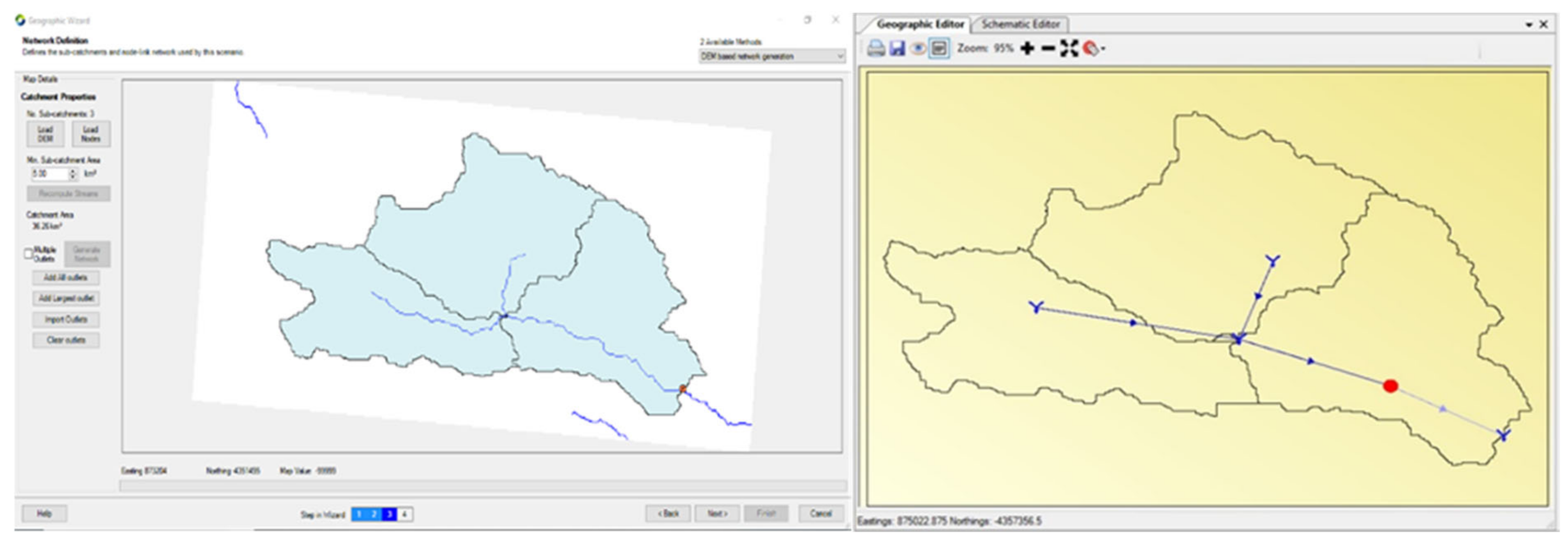
The first step is to prepare a catchment digital elevation model (DEM) that is to be loaded for creating a geographic model in Source [25]; see Figure 2. The DEM can be extracted as an ASC file format from the Geoscience website (Figure 2 in blue) and after processing in QGIS by using Model Fill Sinks, can show the desired catchment boundary (Figure 2 in Yellow). Following this, the catchment outlet is selected by the Shapefile of the QGIS via Source. For the precise location, the coordinate system of the outlet can be identified via Google; it can then be converted to the Source coordinate system. Source itself can draw out the river network system by identifying the minimum number of sub-catchments; for the purpose of this study, three sub-catchments were selected. The next step is to configure the catchment for rainfall–runoff modelling. In this study, the effectiveness of the GR4J, Sacramento and AWBM models in the Source rainfall–runoff framework were assessed. The following sections provide detailed descriptions of these models. The calibration and validation experiments were performed in catchment mode in the Source platform to analyse the efficiency of the above three rainfall–runoff models available in the Source platform for the Painakalac catchment.

2.2.1. GR4J Model

Gr4J is a daily time-step running lumped conceptual model. It has the ability to calculate soil moisture. The GR4j model is an upgraded version of GR3J, which was created by Edijatno and Michel. The model’s origins may be linked back to France, and it has since been researched all around the world [13,26]. It has the advantages of tracking high flow better than the other two models, Sacrament and AWBM [7]; moreover, it takes less time in calibration and validation due to its simplicity. However, this model is not effective in capturing lower flows.
The GR4J rainfall–runoff model produces streamflow by putting the rainfall and evapotranspiration data in the model. The detailed processes of the model and its equations are presented in the reference [27]. The GR4J model generally had four parameters: X1, X2, X3 and X4. However, Source GR4J comprises 6 parameters, including the above four and additionally, K and C (see Table 1 below). These two parameters are used to isolate the base flow and quick flow in the model without affecting the model simulation results. The use of these two parameters is optional [28]. For this study, the default values of K (0.95) and C (0.15) were used [29]. The X1 Parameter is a production store that is located at the surface of the soil, where rainfall can be stored; in addition, evapotranspiration and percolation can happen in this store. The type of store soil can influence the capacity of the store and a small amount of porosity in the soil can increase the size of the production storage. The water exchange coefficient (X2) can influence the routing store, where the negative result caused the water to move to the depth of the aquifer whilst when there was a positive result, the water moved from an aquifer to routing storage. The routing storage X3 is the quantity of water that can be stored into soil voids; the humidity and type of soil can influence routing store capacity. X4 shows the duration of conversion of rainfall to streamflow and is created by the peak of flood hydrograph on the GR4J model [30].

2.2.2. Australian Water Balance Model (AWBM)

The Australian water balance model (AWBM), which was developed in the early 1990s, is one of Australia’s most widely used rainfall–runoff models. Two primary versions of AWBM are available. One version is designed for daily water yield and low flow study, while the other is designed for hourly flood runoff simulation. A version of the daily water yield model for use on ungauged catchments was released in the start of 2003 [31].
This model is a lumped conceptual model primarily designed for river basin management in Australia. The detailed processes of the model and its equations are presented in the reference [32]. The AWBM is a simple rainfall–runoff model that associates rainfall and evapotranspiration to streamflow. This model has five water stores in which three surface stores are used to model partial areas of streamflow while the other two stores are a base flow store and surface streamflow routing store, respectively. Table 2 illustrates the AWBM model parameters and their descriptions. Each partial area has its own storage capacity as C1, C2 and C3. The partial areas A1, A2 and A3 show the modeller defined functional unit or soil classification and the sum of them should be equal to 1. For every time step of the model, the rainfall is put into surface stores; then the evapotranspiration is deducted from each store individually. Excess rainfall is forming as a result of daily rain spills and these rainfalls are distributed between the base flow store and surface routing store. The amount of water to be released to each store is represented by the base flow index (BFI) parameter. The aggregate runoff is based on total surface water and base flow [7]. The base flow recession constant (KBase) calculates the rate of discharge of water from the base flow store while the surface flow recession constant (KSurf) calculates the rate of discharge of water from the surface runoff routing storage [33]. The AWBM rainfall–runoff model produces a better runoff result for larger catchment and medium flows [7] while this model is not so effective in a smaller catchment.

2.2.3. Sacramento Rainfall–Runoff Model

The Sacramento model was developed by Burnash et al. [34] for the United States National Weather Service and the California Department of Water Resources; since then, this modelling tool has been used extensively across the world. Its performance was also enhanced by structurally modifying the model from earlier experiments. The Sacramento model has worked successfully in a variety of climates, including humid, arid and semi-arid conditions [15,34]. This model generates daily runoff by the input of daily rainfall and potential evapotranspiration data. This model has five stores and sixteen parameters to model the runoff, where the stores and parameters are illustrated in Table 6. The detailed processes of the model and its equations are presented in the reference [35]. The Sacramento rainfall–runoff model is considered a complex model compared to the GR4J and AWBM models. The Sacramento model represents the soil as two layers, which are considered conceptually hydrological active zones. The Sacramento model can classify the catchment into permeable and impermeable areas. The impermeable area generates runoff for any type of rainfall whilst the permeable area generates runoff from heavy rainfall. The catchment soil was divided into two layers, where a thin layer is considered in the upper zone while a much thicker layer is considered in the lower zone. The thin layer is comprised of a tension (UZTW) and free water store (UZFW), while the thick layer is comprised of a tension store (LZTW) and two water stores (LZFWP, LZFWS). These tension and free water storages react to produce soil moisture conditions and five elements of runoff [7,36]. In tension water stores, water is accumulated between soil layers via surface tension and water is removed only with the help of evapotranspiration. Whilst in free water storage, water can move in a perpendicular direction and sideways within the soil; in addition, it can be discharged via the upper zone as interflow and in the lower zone as base flow. The depletion coefficients (LZPK, LZSK and UZK) calculate the rate of discharge from these free water storages; the percolation of water from the upper to lower free water stores is determined through the parameters PFREE, REXP and ZPERC. The runoff from the impermeable area is calculated by the PCTIM and ADIMP parameters; the runoff loss through the whole process is calculated through the SIDE, SSOUT and SARVA parameters. The Sacramento model uses the unit hydrographs (UH1-UH5) to show the fraction of flow present at the channel outlet at selected time intervals. The final parameter RSERV is the amount of water in the lower zone free water stores, which is not available for transpiration. The streamflow forecast from the Sacramento model is via a combination of different impermeable areas, surface runoff, interflow and base flow. The impermeable surfaces produce quick runoff from rainfall without a time delay while the time wait can be in days for interflow, weeks for base flow and several months for primary base flow [35]. According to Maolin, the Sacramento model provides a better result in a dry season and when the river has reduced flow; it overestimates the flow during a wet season [15].

2.3. Catchment, Streamflow and Climate Data

For the Painkalac catchment, the streamflow data were taken from station number 235,257, located at a latitude of −38.44 and a longitude of 144.05. The rainfall and PET data are taken from the station located at a latitude of −38.45 and a longitude of 144.05, which is closest to the catchment area.
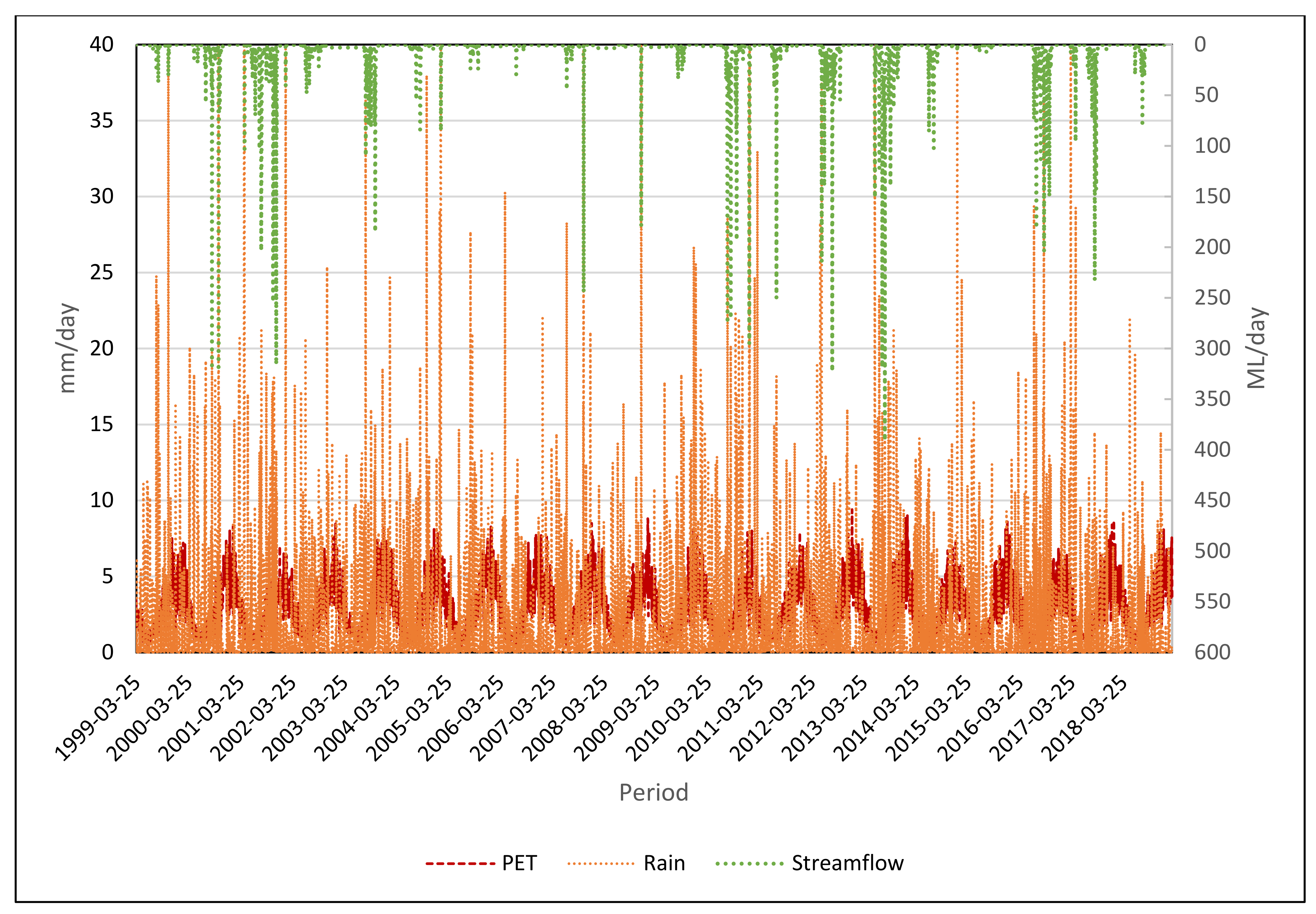
The three major input data for all the models are evapotranspiration (PET), daily rainfall and streamflow. Trend analysis of the data was conducted before the models were run over the configured run time using a single analysis procedure. The required data, such as rainfall and PET data, are obtained from the Queensland Government website [37], while the streamflow data are downloaded from the Bureau of Metrology, Australia (BOM) website. However, these data sets do not have any missing data; this makes the running process smooth. The data for rainfall and potential evapotranspiration are available from the years 1989–2019 while the observed streamflow data is available from 1999–2019. Two-thirds of the available streamflow data were used for calibration while the last one-third of the data was used for validation [11]. Figure 3 below depicts the time series data for the streamflow (from 1999–2019), rainfall and PET (1999–2019). The maximum observed streamflow during 2013 is 391 ML/d. The maximum rainfall during 2005 is 80.70 mm/d while the minimum rainfall is 0.10 mm during 1999. The maximum PET during 2013 is 9.40 mm/d while the minimum PET is 0.30 during 1999.

2.4. Model Calibration and Validation

One of the advantages of the Source platform is auto-grouping the parameters for producing Meta parameters, which allows the user to group the parameters. This could be applied for the whole of the catchment regardless of catchments or functional units; it enables the running of the calibration stage without difficulty. The calibration is performed via many steps, such as uploading streamflow data, selecting objective functions and optimisation methods.
The objective function measures the over goodness-of-fit between the simulated flow and observed flow; thus, it produces the calibration accuracy value of rainfall–runoff models. It also interprets the observed and modelled outputs into a single number [11]. For this study, all the available objective functions were used during the calibration process. They are the Nash–Sutcliffe efficiency (NSE) daily, NSE monthly, NSE monthly and bias penalty, NSE daily and flow duration, NSE daily and log flow duration, NSE daily and bias penalty, NSE log daily and NSE log daily bias penalty. The NSE is a model evaluation coefficient that is widely used in all hydrological (and other) modelling research [28]. The Nash–Sutcliffe efficiency is a normalised calculation that determines the size of residual variance in relation to observed data variance. It measures how well-simulated data matches observed data and runs from −∞ +1, with +1 indicating a perfect fit. As a result, the closer the Nash values are to +1, the better the streamflow prediction and model performance [38]. According to the research of 63 expert hydrologists, NSE monthly values of 0.6 or higher are “usually adequate” for monthly runoff simulations; however, another research by Yu and Zhu [14] adopted an NSE value of 0.7 or greater as acceptable for the performance of model simulation.
The iterative optimisation search algorithm is used for finding the best parameters values of the rainfall–runoff model. The Source model provides two methods for optimisation, which are shuffled complex evolution (SCE) and uniform random sampling. A test analysis was undertaken for more than 200 catchments in south-east Australia and found that there is an advantage for using a local optimiser (Rosenbrock) after a global optimiser (SCE) for adjusting a calibrated parameter [11]. The SCE algorithm is an efficient global optimiser that tries to search the entire perimeter space and can be slow for large models. The second algorithm, Rosenbrock, is a gradient-based virtual algorithm; it is a local optimiser and is quicker [39]. In this study, the SCE following the Rosenbrock optimisation method was used for the model development. The combination of these two algorithms speeds up the optimisation processes [40]. The simulation is then used in the final stage by utilising the best parameter set, which is determined by objective functions.
During the validation process, the calibrated model parameter is used to simulate runoff for an independent period different from the calibration period. The validation step confirms the ability of the model to forecast streamflow outside the calibration period [41]. Hence, the Source model uses the calibrated parameters of the rainfall–runoff model for the validation steps; further observed and modelled flow can be compared. A validation accuracy value can be observed as well.

3. Model Results

The above said three models, AWBM, GR4J and Sacramento, were calibrated using Source version 4.7.0 for the Painkalac catchment. The calibration and validation accuracy results for the three utilised rainfall–runoff models for the Painkalac catchment with different objective functions are shown in Table 3. The purpose of using all the available objective functions and all the optimisation methods was: to select the best objective function and optimisation method for attaining higher calibration and validation accuracy values for the models; and finally, to estimate a good runoff volume. From Table 3, the NSE log daily objective function produces the best result (higher NSE) for the selected three models. It is clear that GR4J is performing better compared to AWBM or Sacramento in both the calibration and validation periods. The GR4J rainfall–runoff model performed better in all the statistical parameters. The NSE value was 0.54 for AWBM, 0.65 for Sacramento and 0.74 NSE for the GR4J model. During the validation process, GR4J also performed better in terms of NSE log daily than AWBM and Sacramento, which was above 0.85. According to the obtained results, all of the models provide positive results for the Painakalac catchment in this study. However, it is learned that the GR4J model performs better in terms of calibration accuracy value and prediction compared to the Sacramento and AWBM models. Based on this result, the GR4J model was selected to study different scenarios (land-use change, climate change and combined land-use and climate change impact on streamflow forecast) using NSE log daily as an objective function.
Further comparisons of these models are shown in Table 4, where the GR4J model again performed better in all the univariate statistics, such as mean and standard deviation. Since the NSE log daily objective function focuses on the lower flow [42], the standard deviation and mean values are lower than the observed flow. The statistical characteristics of the observed and simulated discharges with all three models are summarised in Table 4.

3.1. Calibration and Validation of Selected Models

The calibrated parameters are produced after the calibration of a model, where the default parameter values of the rainfall–runoff models are optimised. The calibrated parameters of each rainfall–runoff model were compared with the default parameters and discussed in the sections below.

3.1.1. AWBM Model Calibration and Validation

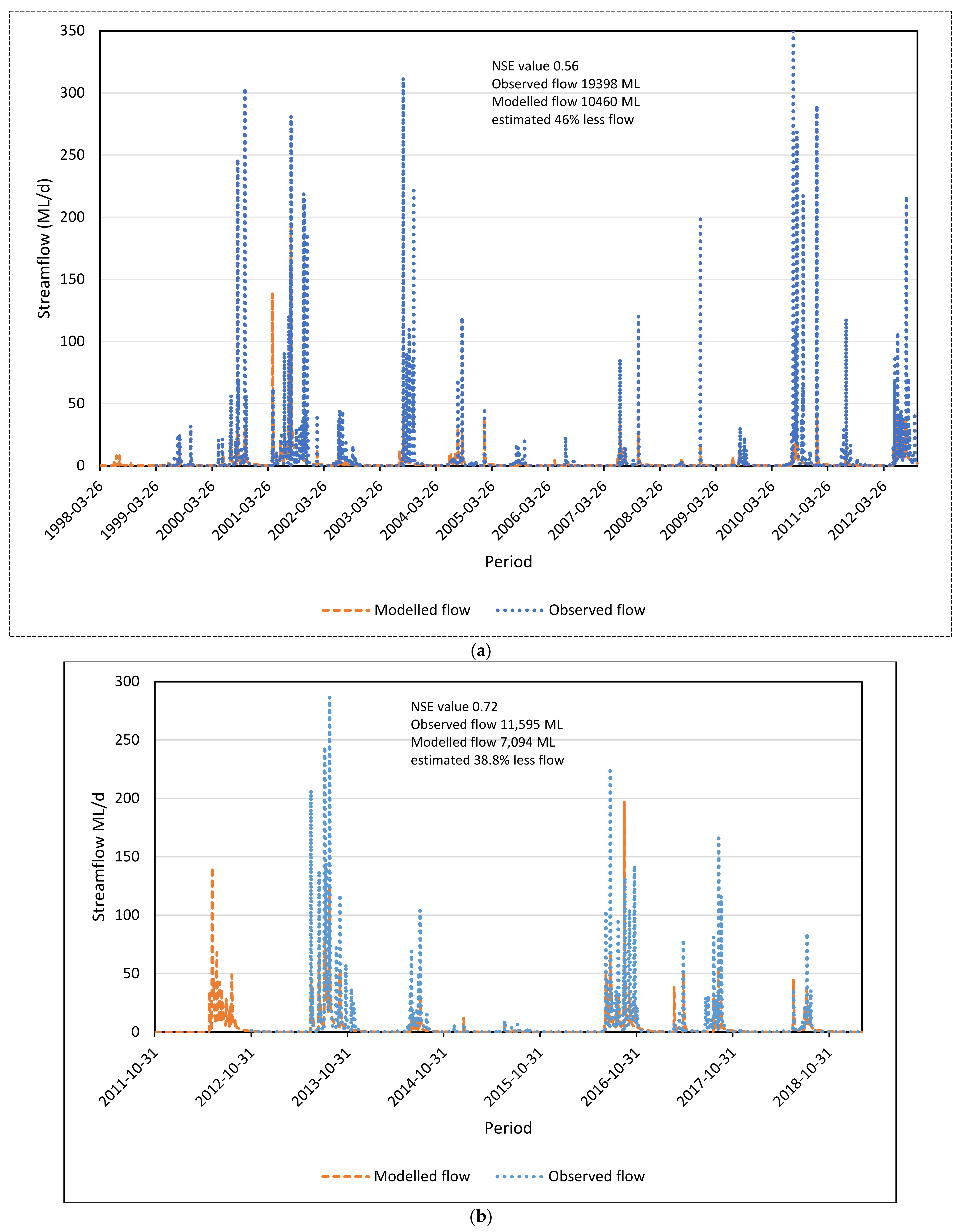
For this model, the calibration period is from 26 March 1999 (the available two-thirds of the observed data) to 30 October 2012; the objective function used NSE log daily. The calibrated parameter of the AWBM rainfall–runoff model is shown in Table 5. It can be seen from Figure 4a that the modelled flow for calibration was estimated as less compared to the observed flow; the actual observed flow is 19,398 ML while the predicted modelled flow is 10,460 ML, which is approximately 46% less than the observed flow. In addition, the calibration accuracy value is 0.56 (see Table 5). This shows that the quality of the model is not acceptable while according to hydrologists, an NSE of 0.6 or more provides adequate model performance [28].
The validation period is from 31 October 2012 to 4 March 2019. It can be seen from Figure 4b that the validation accuracy value is 0.72 and the predicted modelled flow is around 38.8% less than the observed flow; this shows that the AWBM model estimated an acceptable flow for the validation period.

3.1.2. Sacramento Model Calibration and Validation

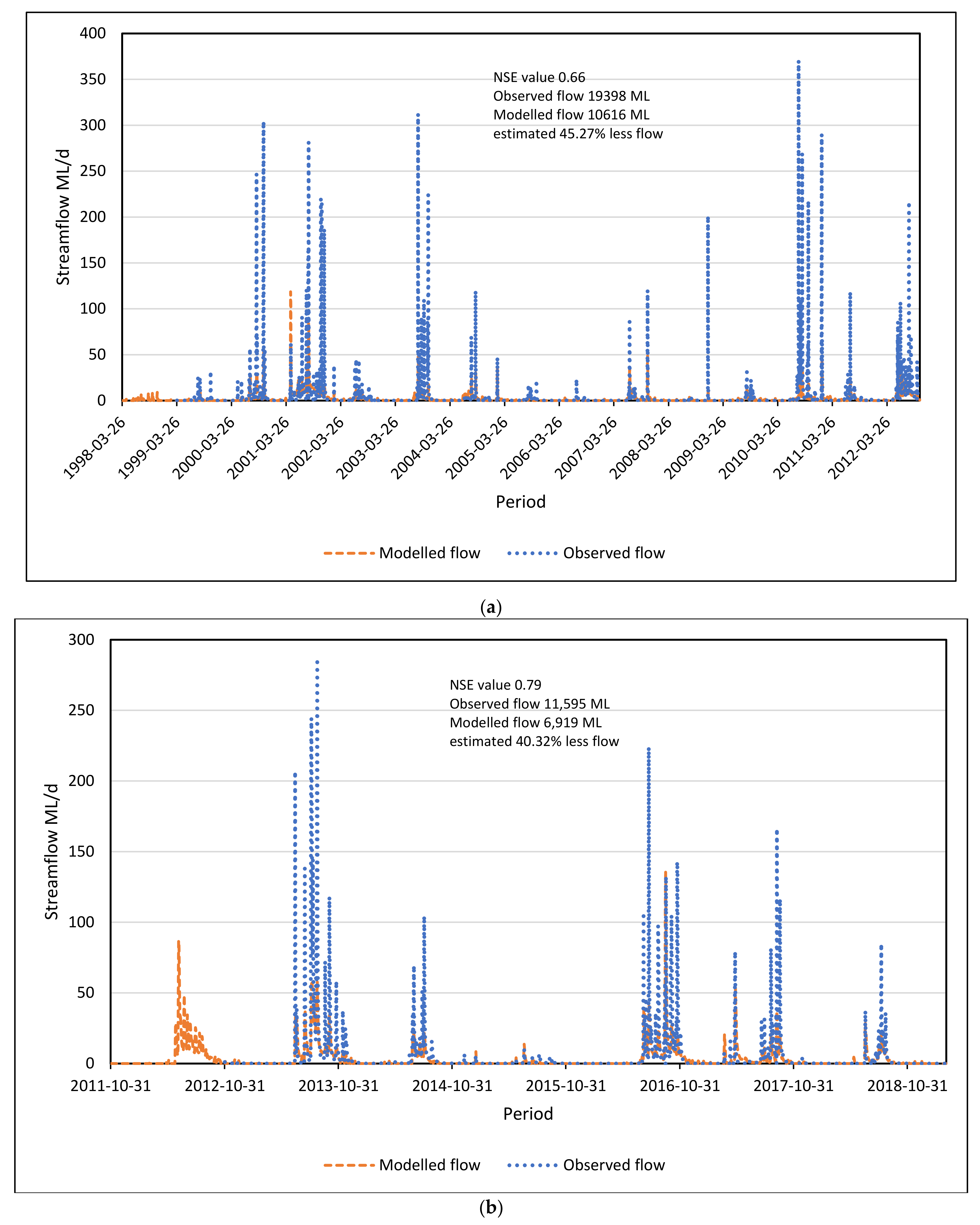
The calibration period for the Sacramento model is similar to the AWBM model, which is from 26 March 1999 to 30 October 2012. The model produced a calibration accuracy value of 0.66; in addition, the modelled flow underestimated approximately 45.27% less streamflow, which can be seen from Figure 5a. The calibration accuracy value suggests that the model performance is better compared to the AWBM model [28]; however, for catchment water modelling, the higher and closer the NSE value is to 1, the better the model performs. The calibrated parameters are shown below in Table 6 below. The validation period for the Sacramento model is 31 October 2012 to 4 March 2019 (the remaining one-third of the data). The model estimated the validation accuracy value as 0.79 and the estimated modelled flow as around 40.32% less compared to the observed flow (see Figure 5b). The NSE value shows that the model is capable of estimating flow outside the calibration period.

3.1.3. GR4J Model Calibration and Validation

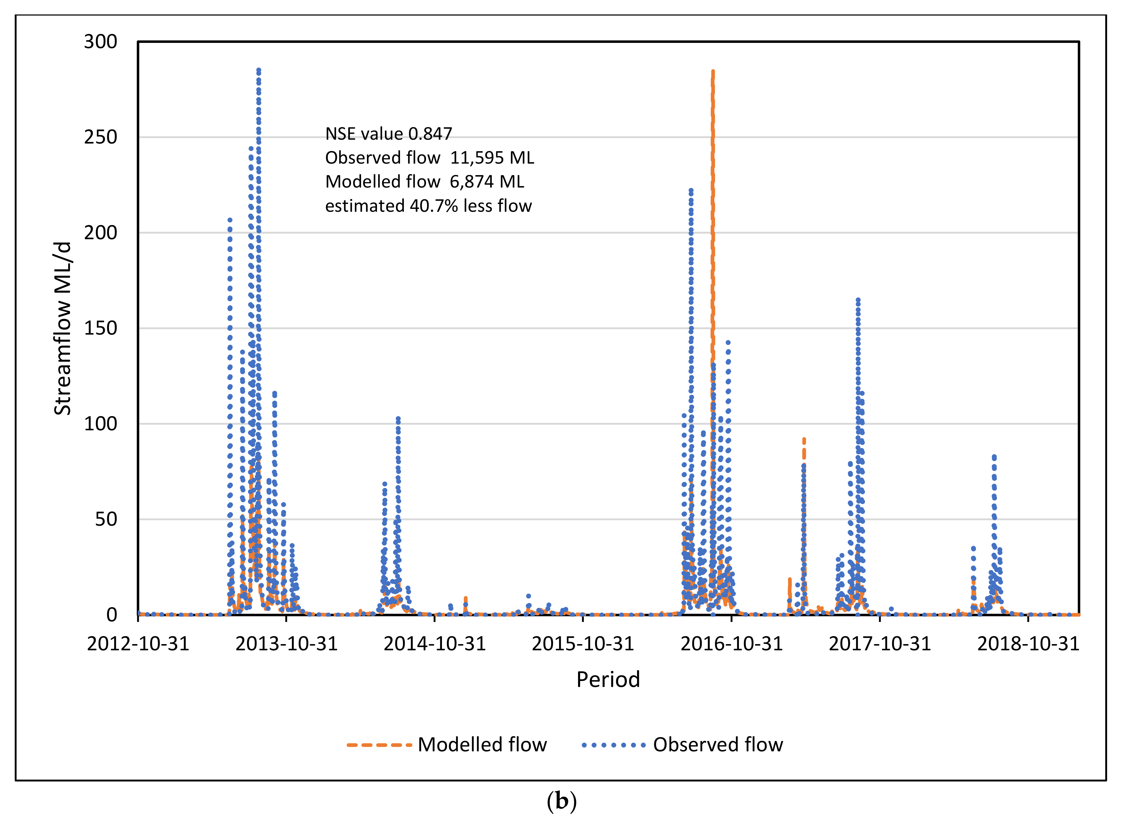
Figure 6a compares the modelled vs. observed flow for the calibration of the GR4J model. The model produced a calibration accuracy value of 0.74 and predicted 45.7% less flow compared to the observed flow. The NSE value shows the model is very good for water quantity simulation [28] and this model produced the higher calibration accuracy value among the other three models; thus, this model is the most suitable model for the Painkalac catchment. The calibrated parameters of this model are present in Table 7 below. The validation chart for the GR4J model can be seen in Figure 6b. The produced validation accuracy value for this model is 0.84 and the model estimated 40.7% less streamflow compared to the observed flow. The NSE value indicates the model has the best capability to predict streamflow outside the calibration period. Therefore, this model is selected as the most suitable model for the Painkalac catchment for the analysis of further scenarios.
The GR4J rainfall–runoff model produced the highest calibration and validation accuracy values of the three models; therefore, the GR4J rainfall–runoff model was selected for catchment streamflow assessment under various scenarios. However, none of the models performed well under peak streamflow values.

3.2. GR4J Model Application under Different Scenarios

The GR4J rainfall–runoff model was used for analysing different scenario impacts.
The following scenarios were developed for hydrologic modelling:
(A)
Land use change in the case study catchment from forest land to agricultural land use.
(B)
Climate change impacts.
(C)
Combined land use and climate change impacts.
The modelled flow for these scenarios will help the water management authority to take informed decisions for the better operation and management of the catchment when there is land use or climate change or both occur simultaneously.

3.2.1. Land Use Change Impact

Painkalac catchment is located within the Corangamite region, where more than 70% of the land is used for agriculture; this is considered the third-largest source of income after industry and tourism in this region [18]. Therefore, 50% of the functional units of the two sub-catchments within the Painkalac catchment were converted from forest land to agricultural land in order to observe the impacts of land-use change on the selected model. After model simulation, the land-use change (addition of agricultural land) resulted in 42.26% less water compared to the observed flow (Table 8).
Agricultural land, shrub land and grassland areas are prone to a combination of decreasing rainfall and increasing temperature and solar radiation; this results in drier conditions, less runoff and ultimately produces less runoff from the catchment while forested areas are strong under those conditions [43].
The parameters of the rainfall–runoff models before and after the land-use change are shown in Table 9. The rainfall–runoff model parameters, the maximum capacity of the production store (X1) and the ground store exchange coefficient (X2), were reduced because the capacity of holding water in the production store decreased. This was due to exposure to a higher temperature and solar radiation happening in this store as compared to forest land; however, the reduced X2 shows more water is stored to aquifer due to a higher negative value [30]. The value of the X3 parameter shows that a higher amount of water is stored into soil voids. Finally, the X4 parameter is slightly high due to more water being available in this process as compared to forest land, and due to slightly more time to convert from rainfall to runoff.
Furthermore, the Painkalac catchment is relatively small (36 Km2) and only two sub-catchments are exposed to 50% (6.61 Km2 + 5.13 Km2 =11.75 Km2) land-use change; thus, there was not much flow change between the modelled flow under the existing conditions and the modelled flow after the land-use change. The land-use change impacted about 1.54% less flow compared to the modelled flow under the existing conditions (Table 8).

3.2.2. Higher Climate Change Scenario

Victoria’s climate is considered to change in the future due to climate change; this could impact Victoria’s water resources, which are mostly dependent on the climate. Climate change could reduce water availability in the future due to drought, which can cause a problem in the planning, operation and management of water resources. Therefore, the need for a short-term water quantity forecasting model is important for better daily and monthly water resources management. However, this model is also capable of forecasting streamflow for any period of time in the future as long as sufficient data are available. According to the global climate model projections data developed by the DELWP climate change guidelines, there will be a change in temperature, potential evapotranspiration (PET) and rainfall for the years 2040 and 2065. The temperature is expected to increase by 2.5 °C in the Painkalac catchment, which, in turn, would increase the PET by 9.5%; rainfall is expected to decrease by 19% in the year 2065 [4].
For higher climate change scenarios, the model was calibrated to analyse the impact of climate change against the existing conditions. The calibrated parameter is shown in Table 10 below. After the model simulation, the impact of climate change on streamflow can be seen below in Table 11; as expected, there will be approximately 45.68% less streamflow by 2065 due to the higher climate impact.

3.2.3. Combined Land-Use and Higher Climate Change Scenario

In this scenario, the GR4J model was subjected to a combined land use and higher climate change scenario in order to evaluate the impact on streamflow. The calibrated parameters of this model are shown in Table 12. The impact on streamflow due to the combined land use and higher climate change scenario is shown in Table 13. It is expected that there will be approximately 48.06% less streamflow compared to the observed flow by 2065 due to combined land use and a higher climate change effect.

4. Conclusions

For the Painkalac catchment, three different rainfall–runoff models, such as GR4J, Sacramento and AWBM, were evaluated in terms of model performance. All three models were calibrated and validated with the eight objective functions available in order to select the most suitable model with the help of higher calibration and validation accuracy values. It was found that the GR4J rainfall–runoff model with the NSE log daily objective function produced the highest calibration value of 0.74 and validation accuracy value of 0.84.
The GR4J model was used as a baseline model; then, the impact of different scenarios, such as climate change, land-use change and combined land-use and climate change scenarios, were evaluated for streamflow. The climate change for the year 2065 will result in approximately 45.678% less streamflow in the reservoir and the land-use change alone would result in approximately 42.26% less flow; the combined land use and climate change would result in 48.06% less flow compared to the observed flow. The developed model can be used for short-term forecasting for up to three months by using the predicted PET and rainfall data obtained from the BOM website; this can enhance the daily operation and management of the Painkalac Creek catchment. However, to further improve the model accuracy value, manual calibration and sensitivity analysis is recommended.
It is recommended that water professionals should investigate the suitability of the rainfall–runoff models using the developed methodology for a particular catchment considering the characteristics of the catchment and available streamflow data. The investigation can be extended to the wider rainfall–runoff models available using the proposed methodology.

Author Contributions

Conceptualization, N.Z., C.M. and S.M.; methodology, V.M.J. and S.M.; writing—original draft preparation, N.Z.; writing—review and editing, N.Z., V.M.J., S.M., A.S. and D.N.; supervision, C.M. and S.M. All authors have read and agreed to the published version of the manuscript.

Funding

This research received no external funding.

Institutional Review Board Statement

Not required.

Informed Consent Statement

Not applicable.

Data Availability Statement

Not applicable.

Acknowledgments

The authors would like to acknowledge the Bureau of Meteorology, Barwon Water and eWater for providing the necessary data for this study. The authors acknowledge the funding support received from the Institute for Sustainable Industries and Liveable Cities (ISILC) for the article publishing fee.

Conflicts of Interest

The authors declare no conflict of interest.

References

  1. Vaze, J.; Chiew, F.; Perraud, J.-M.; Viney, N.; Post, D.; Teng, J.; Wang, B.; Lerat, J.; Goswami, M. Rainfall-runoff modelling across southeast Australia: Datasets, models and results. Australas. J. Water Resour. 2011, 14, 101–116. [Google Scholar] [CrossRef]
  2. De Vos, N.; Rientjes, T. Multi-objective performance comparison of an artificial neural network and a conceptual rainfall—Runoff model. Hydrol. Sci. J. 2007, 52, 397–413. [Google Scholar] [CrossRef]
  3. Dwarakish, G.; Ganasri, B. Impact of land use change on hydrological systems: A review of current modeling approaches. Cogent Geosci. 2015, 1, 1115691. [Google Scholar] [CrossRef]
  4. DELWP. Guidelines for Assessing the Impact of Climate Change on Water Supplies in Victoria. 2016. Available online: https://www.water.vic.gov.au/__data/assets/pdf_file/0014/52331/Guidelines-for-Assessing-the-Impact-of-Climate-Change-on-Water-Availability-in-Victoria.pdf (accessed on 13 April 2021).
  5. Legesse, D.; Vallet-Coulomb, C.; Gasse, F. Hydrological response of a catchment to climate and land use changes in Tropical Africa: Case study South Central Ethiopia. J. Hydrol. 2003, 275, 67–85. [Google Scholar] [CrossRef]
  6. Leavesley, G.H. Modeling the effects of climate change on water resources—A review. Assess. Impacts Clim. Chang. Nat. Resour. Syst. 1994, 28, 159–177. [Google Scholar]
  7. Kunnath-Poovakka, A.; Eldho, T. A comparative study of conceptual rainfall-runoff models GR4J, AWBM and Sacramento at catchments in the upper Godavari river basin, India. J. Earth Syst. Sci. 2019, 128, 33. [Google Scholar] [CrossRef]
  8. Chiew, F.; Peel, M.; Western, A. Application and testing of the simple rainfall-runoff model SIMHYD. In Mathematical Models of Small Watershed Hydrology and Applications; Water Resources Publications: Highlands Ranch, CO, USA, 2002; pp. 335–367. Available online: https://wrpllc.com/books/mmsw.html (accessed on 30 June 2022).
  9. Carr, R.; Podger, G. eWater Source-Australia’s next generation IWRM modelling platform. In Proceedings of the Hydrology and Water Resources Symposium 2012, Sydney, NSW, Australia, 19–22 November 2012; p. 742. [Google Scholar]
  10. Dutta, D.; Welsh, W.D.; Vaze, J.; Kim, S.S.; Nicholls, D. A comparative evaluation of short-term streamflow forecasting using time series analysis and rainfall-runoff models in eWater source. Water Resour. Manag. 2012, 26, 4397–4415. [Google Scholar] [CrossRef]
  11. Vaze, J.; Jordan, P.; Beecham, R.; Frost, A.; Summerell, G. Guidelines for Rainfall-Runoff Modelling: Towards Best Practice Model Application; eWater CRC: Clayton, VIC, Australia, 2011. [Google Scholar]
  12. Bennett, J.C.; Robertson, D.E.; Ward, P.G.; Hapuarachchi, H.P.; Wang, Q. Calibrating hourly rainfall-runoff models with daily forcings for streamflow forecasting applications in meso-scale catchments. Environ. Model. Softw. 2016, 76, 20–36. [Google Scholar] [CrossRef]
  13. Anshuman, A.; Kunnath-Poovakka, A.; Eldho, T. Performance evaluation of conceptual rainfall-runoff models GR4J and AWBM. ISH J. Hydraul. Eng. 2021, 27, 365–374. [Google Scholar] [CrossRef]
  14. Yu, B.; Zhu, Z. A comparative assessment of AWBM and SimHyd for forested watersheds. Hydrol. Sci. J. 2015, 60, 1200–1212. [Google Scholar] [CrossRef]
  15. Zhang, M.; Wang, J.; Huang, Y.; Yu, L.; Liu, S.; Ma, G. A new Xin’anjiang and Sacramento combined rainfall-runoff model and its application. Hydrol. Res. 2021, 52, 1173–1183. [Google Scholar] [CrossRef]
  16. Akhter, M.S.; Hewa, G.A. The use of PCSWMM for assessing the impacts of land use changes on hydrological responses and performance of WSUD in managing the impacts at Myponga catchment, South Australia. Water 2016, 8, 511. [Google Scholar] [CrossRef]
  17. Gamage, S.; Hewa, G.; Beecham, S. Modelling hydrological losses for varying rainfall and moisture conditions in South Australian catchments. J. Hydrol. Reg. Stud. 2015, 4, 1–21. [Google Scholar] [CrossRef]
  18. CCMA. Corangamite Regional Catchment Strategy 2013–2019. Available online: https://ccma.vic.gov.au/wp-content/uploads/2021/04/CCMA-RCS-FINAL-JUNE-2013-3.pdf (accessed on 20 April 2021).
  19. Johnson, G. Recreation at the Painkalac Reservoir. Available online: https://aireys-inlet.org/recreation-at-the-painkalac-reservoir/ (accessed on 10 May 2021).
  20. Forsyth, D.A. Report on a Land Use Determination for the Painkalac Creek Water Supply Catchment. Available online: http://vro.agriculture.vic.gov.au/dpi/vro/coranregn.nsf/0d08cd6930912d1e4a2567d2002579cb/99316709e41717c1ca2578760002865a/$FILE/lud_painkalac_creek.pdf (accessed on 15 April 2021).
  21. Raducan, G.M. The Impact of Bushfires on Water Quality; RMIT University: Melbourne, Australia, 2018. [Google Scholar]
  22. Geotechnical, A.S.M. Corangamite Catchment Management Authority Land Use. Available online: https://www.ccmaknowledgebase.vic.gov.au/soilhealth/resource/maps_reports/pdf_maps/factors/ccma/ccma_factors_land_use_mga54.pdf (accessed on 9 March 2021).
  23. eWater Source. A Platform for Truly Integrated Water Resource Management. Available online: https://ewater.org.au/products/ewater-source/why-use-source/ (accessed on 19 April 2021).
  24. eWater. Source Training Course Details. Available online: https://ewater.org.au/products/ewater-source/training/source-training-course-details/ (accessed on 19 April 2021).
  25. Team City. Geographic Wizard for Catchment. Available online: https://wiki.ewater.org.au/display/SD33/Geographic+Wizard+for+catchments (accessed on 10 July 2021).
  26. Demirel, M.C.; Booij, M.J.; Hoekstra, A.Y. The skill of seasonal ensemble low-flow forecasts in the Moselle River for three different hydrological models. Hydrol. Earth Syst. Sci. 2015, 19, 275–291. [Google Scholar] [CrossRef]
  27. Team City. GR4J-SRG. Available online: https://wiki.ewater.org.au/display/SD41/GR4J+-+SRG (accessed on 20 April 2021).
  28. Rezaie, H.; Jabbari, A.; Behmanesh, J.; Jarihani, B.; Hessari, B. Evaluation of SURM and GR4J rainfall runoff models, for theNazloo River catchment in northwest ofIran. World J. Environ. Biosci. 2014, 5, 2277–8047. [Google Scholar]
  29. eWater Source. Observed Catchment Runoff Depth Model. Available online: https://wiki.ewater.org.au/display/SD50/Observed+catchment+runoff+depth+-+SRG (accessed on 20 April 2021).
  30. Harlan, D.; Wangsadipura, M.; Munajat, C.M. Rainfall-Runoff Modeling of citarum hulu river basin by using GR4j. In Proceedings of the World Congress on Engineering, London, UK, June 30–July 2 2010; Volume II, pp. 1607–1611. [Google Scholar]
  31. Boughton, W. The Australian water balance model. Environ. Model. Softw. 2004, 19, 943–956. [Google Scholar] [CrossRef]
  32. Team City. Australian Water Balance Model (AWBM)-SRG. Available online: https://wiki.ewater.org.au/display/SD45/Australian+Water+Balance+Model+%28AWBM%29+-+SRG (accessed on 25 April 2021).
  33. Walter Boughton and Francis Chiew. Calibrations of the Awbm for Use on Ungauged Catchments. 2003, p. iiii. Available online: https://www.ewater.org.au/archive/crcch/archive/pubs/pdfs/technical200315.pdf (accessed on 29 June 2022).
  34. Burnash, R.J.; Ferral, R.L.; McGuire, R.A. A Generalized Streamflow Simulation System: Conceptual Modeling for Digital Computers; US Department of Commerce, National Weather Service, and State of California: Sacrametno, CA, USA, 1973. [Google Scholar]
  35. Team City. Sacramento Model-SRG. Available online: https://wiki.ewater.org.au/display/SD45/Sacramento+Model+-+SRG (accessed on 26 April 2021).
  36. Anderson, R.M.; Koren, V.I.; Reed, S.M. Using SSURGO data to improve Sacramento Model a priori parameter estimates. J. Hydrol. 2006, 320, 103–116. [Google Scholar] [CrossRef]
  37. Queensland Governament. Australian Climate Data from 1889 to Yesterday. Available online: https://www.longpaddock.qld.gov.au/silo/ (accessed on 12 May 2021).
  38. Chiew, F.; McMahon, T. Assessing the adequacy of catchment streamflow yield estimates. Soil Res. 1993, 31, 665–680. [Google Scholar] [CrossRef]
  39. Rosenbrock, H. Some general implicit processes for the numerical solution of differential equations. Comput. J. 1963, 5, 329–330. [Google Scholar] [CrossRef]
  40. Blakers, R. Calibration for Catchment Modelling. Available online: https://www.youtube.com/watch?v=F8J_azPoUfs&t=1306s (accessed on 13 May 2021).
  41. Black, D.; Wallbrink, P.; Jordan, P.; Waters, D.; Carroll, C.; Blackmore, L. Guidelines for Water Management Modelling: Towards Best-Practice Model Application; eWater Cooperative Research Centre: Clayton, VIC, Australia, 2011. [Google Scholar]
  42. Blakers, R. Bivariate Statistics SRG. Available online: https://wiki.ewater.org.au/display/SD41/Bivariate+Statistics+SRG#BivariateStatisticsSRG-NSEofLogData (accessed on 27 April 2021).
  43. Farinosi, F.; Arias, M.E.; Lee, E.; Longo, M.; Pereira, F.F.; Livino, A.; Moorcroft, P.R.; Briscoe, J. Future climate and land use change impacts on river flows in the Tapajós Basin in the Brazilian Amazon. Earth Future 2019, 7, 993–1017. [Google Scholar] [CrossRef]
Figure 1. (a) Location and area map of the Painkalac catchment; (b) land-use map of the Painkalac catchment adapted from [22].
Water 14 02523 g001
Figure 2. Depiction of the drainage lines of the Painkalac catchment.
Water 14 02523 g002
Figure 3. PET, rainfall and observed streamflow time series chart.
Water 14 02523 g003
Figure 4. (a) AWBM model calibration; (b) AWBM model validation.
Water 14 02523 g004
Figure 5. (a) Sacramento model calibration; (b) Sacramento model validation.
Water 14 02523 g005
Figure 6. (a) GR4J model calibration; (b) GR4J model validation.
Water 14 02523 g006aWater 14 02523 g006b
Table 1. Parameters in GR4J and their default values are adapted from [27].
Parameter DescriptionUnitsDefaultRange
X1Capacity of the production soil (SMA) store mm3501–1500
X2Water exchange coefficient none0−10.0–5.0
X3Capacity of the routing storemm401–500
X4Time parameter for unit hydrographsdays0.50.5–4.0
KFilter parameter (as in the observed catchment runoff depth model)none0.950–1
CShape parameter (as in the observed catchment runoff depth model)none0.150–1
Table 2. Parameters in AWBM and their default values adapted from [32].
ParameterExplanationUnitsDefault
A1Fractional area of surface store 1 (part of the catchment) 0.134
A2Fractional area of surface store 2 (part of the catchment) 0.433
A3Fractional area of surface store 3 (part of the catchment) 0.433
C1Capacity surface store 1mm7
C2Capacity surface store 2 mm70
C3Capacity surface store 3mm150
BF1 Base flow index (portion of extra runoff going into the base flow store) 0.35
KBaseBase flow recession constant (portion of moisture depth left as per time-step) 0.95
KSurfSurface flow recession constant (portion of moisture depth left as per time-step) 0.35
Table 3. The comparison of the three models, GR4J, AWBM and Sacramento, for the calibration and validation accuracy values.
AWBM Rainfall–Runoff ModelSacramento Rainfall–Runoff ModelGR4J Rainfall–Runoff Model
Objective FunctionsCalibration
Accuracy
Validation
Accuracy
Calibration
Accuracy
Validation
Accuracy
Calibration
Accuracy
Validation
Accuracy
NSE daily and flow duration 0.500.690.590.720.620.61
NSE daily and log flow duration0.510.690.630.660.370.25
NSE daily0.210.470.350.520.370.40
NSE monthly0.520.810.620.830.720.79
NSE daily and bias penalty 0.19N/A0.330.520.320.39
NSE monthly and bias penalty0.480.790.620.820.690.78
NSE log daily0.560.720.660.790.740.84
NSE log daily bias penalty0.500.670.560.720.700.68
Table 4. Comparison of the three-model performance predicted by univariate statistics.
Objective FunctionCalibration/Validation PeriodAttributeAWBMSacramentoGR4JObservedPerfect Model Situation
NSE log daily26 March 1999–30 October 2012 (calibration)Nash–Sutcliff efficiency0.560.660.74 1
Mean (ML/d)2.102.132.123.90
Standard deviation (ML/d)7.125.918.7717.82
NSE log dailyValidation period
31 October 2012 to 4 March 2019 (validation)
Nash–Sutcliff efficiency0.720.790.84 1
Mean (ML/d)3.0632.982.965.00
Standard deviation (ML/d)10.0818.2210.8518.94
Table 5. Calibrated parameters of the AWBM rainfall–runoff model.
Objective Function ParametersDefault Values Calibrated Parameters Parameters Range
NSE log DailyA10.130.110–1
A20.430.200–1
KBase0.950.670–1
KSurf0.350.980–1
BFI0.350.510–1
C1749.790–50
C270109.220–200
C370191,3120–500
Calibration accuracy0.560–1
Validation accuracy0.720–1
Table 6. Calibrated parameters of the Sacramento rainfall–runoff model.
Objective Function ParametersDescriptionDefault ValuesCalibrated ParametersParameters Range
NSE log DailyLZTWMLower zone tension water maximum: only evapotranspiration can remove water form this store.13096.3875–300
LZFSMLower zone free water supplemental maximum: the largest volume from which a supplemental base flow can be obtained.25119.3315–300
LZFPMLower zone free water primary maximum: the maximum capacity from which a primary base flow can be extracted.6060040–600
LZSKThe amount of water in LZFSM that drains as a daily base flow.0.050.030.03–0.20
LZPKThe amount of water in LZPK that drains as a daily base flow.0.010.010.001–0.015
RSERVThe percentage of free water in the lower zone that is not accessible for transpiration.0.30.200–0.40
SIDEThe ratio of non-channel base flow (deep recharge) to channel (visible) base flow.00.800–0.80
UH1The first component of the unit hydrograph, i.e., the fraction of simultaneous runoff that has not been delayed.10.330–1
UH2The second component of the unit hydrograph, i.e., the fraction of instantaneous runoff that has slowed down by one time step.010–1
UH3The third component of the unit hydrograph, i.e., the fraction of instantaneous runoff that has slowed down by two time steps.010–1
UH4The fourth component of the unit hydrograph, i.e., the fraction of instantaneous runoff that has slowed down by three time steps.00.700–1
UH5The fifth component of the unit hydrograph, i.e., the fraction of instantaneous runoff that has slowed down by four time steps.00.570–1
UZTWMUpper zone tension water maximum: the maximum volume of water stored by the top zone between the field capacity and wilting point that can be lost from the soil surface by direct evaporation and evapotranspiration. Before any water in the top zone is moved to other storages, this storage gets filled.5051.1425–125
UZFWMUpper zone free water maximum: this store serves as both a source of water for interflow and a driving force for water transfer to deeper levels.407510–75
UZKThe percentage of water in UZFWM that drains as interflow on a daily basis.0.30.470.2–0.5
ZPERCThe maximal percolation rate is defined as a proportional rise in PBase.403000–80
REXPAn exponent that determines the rate of change in the percolation rate as lower zone water storage changes.13.090–3
PCTIMThe portion of the basin that is continuously impermeable and is adjacent to stream channels, contributing to direct runoff.0.010.010–0.05
SARVAA decimal fraction that represents the portion of the basin that is generally covered by streams, lakes and vegetation that can cause evapotranspiration to reduce streamflow.00.020–0.10
SSOUTThe amount of flow that can be carried by porous material in the streambed.00.010–0.10
ADIMPThe portion of the catchment that develops impermeable qualities as a result of soil saturation.00.200–0.20
PFREEThe lowest amount of percolation from the higher to lower zone that is immediately available for refilling the lower zone’s free water storage.0.060.390–0.50
Calibration accuracy0.660–1
Validation accuracy0.790–1
Table 7. Calibrated parameters of the GR4J rainfall–runoff model.
Objective FunctionParametersDefault ValuesCalibrated ParametersParameters Range
NSE log DailyX1More information on these parameters can be found in Table 1.350233.031–1500
X20−4.15−10–5
X34019.141–500
X40.51.720.50–4
K0.950.950–1
C0.150.150–1
Calibration accuracy0.740–1
Validation accuracy0.840–1
Table 8. Before and after the land-use change water quantity data.
Observed and Modelled Flow PeriodObserved Flow MLModelled Flow (Original) MLModelled Flow Land-Use Change (Addition of Agriculture) ML
2012–201911,59568746694
40.71%42.26%
Table 9. The parameters of the rainfall–runoff models before and after land-use change.
Objective FunctionParametersModelled (Original) Modelled (Addition of Agriculture)Parameters Range
NSE Log DailyX1More information on these parameters can be found in Table 1.160.67157.051–1500
X2−3.70−4.01−10–5
X320.1620.991–500
X41.391.390.5–4
K0.950.950–1
C0.150.150–1
Model accuracy value 0.840.840–1
Table 10. The parameters of the rainfall–runoff models before and after climate change.
Objective FunctionParametersModelled (Original) Modelled (Addition of Agriculture)Parameters Range
NSE Log DailyX1160.67135.811–1500
X2−3.70−0.52−10–5
X320.169.261–500
X41.391.160.5–4
K0.950.950–1
C0.150.150–1
Model accuracy value0.840.810–1
Table 11. Before and after climate change water quantity result.
Observed data period 2012–2019Percentage % difference in the observed and modelled flow
Observed flow 11,595 ML
Modelled flow existing condition6874 MLDecreased 40.71
Modelled flow for higher climate change6298 MLDecreased 45.67
Table 12. The parameters of the rainfall–runoff models before and after combined land use and climate change.
Objective FunctionParametersModelled Parameters
(Original)
Modelled Parameters
(Combined Land Use and Climate Change)
Parameters Range
NSE Log DailyX1160.67151.291–1500
X2−3.70−0.45−10–5
X320.168.621–500
X41.391.370.5–4
K0.950.950–1
C0.150.150–1
Model accuracy value0.840.810–1
Table 13. Streamflow before and after the combined land-use and climate change result.
Observed data period 2012–2019Percentage % difference in the observed and modelled flow
Observed flow11,595 ML
Modelled flow existing condition6874 MLDecreased 40.71
Modelled flow for land use and higher climate change6022 MLDecreased 48.06
Publisher’s Note: MDPI stays neutral with regard to jurisdictional claims in published maps and institutional affiliations.