
Joint Modelling of Flood Hydrograph Peak, Volume and Duration Using Copulas—Case Study of Sava and Drava River in Croatia, Europe


Abstract
:1. Introduction
2. Data and Methods
2.1. Study Area and Data
2.2. Flood Characteristics
- Divide the mean daily discharge data into non-overlapping blocks of N days and calculate the minima for each of these blocks, and let them be called Q1, Q2, Q3, … Qi.
- Consider in turn (Q1, Q2, Q3), (Q2, Q3, Q4), … (Qi − 1, Qi, Qi + 1), etc.
- In each case, if 0.9·Qi < Qi − 1 and 0.9·Qi < Qi + 1, then the central value is an ordinate for the baseflow line. Continue the procedure until a derived set of baseflow ordinates QB1, QB2, QB3, … QBn is provided with different time periods between them.
- Apply linear interpolation between each QBi value and estimate each daily value of QB1 … Q1.
- If QBi > Qi, then set QBi = Qi.

| Baseflow Separation Method | Acronym | Reference |
|---|---|---|
| Baseflow index method | BFI | Gustard et al. [61]; Koffler and Laaha [63] |
| Recursive digital filter method | RDF1 | Lyne and Hollick [64] |
| RDF2 | ||
| RDF3 | ||
| Sliding interval method | HYSEP1 | Sloto and Crouse [70]; Source code available at: https://github.com/USGS-R/DVstats/blob/main/R/hysep.R, accessed on 1 June 2022 |
| Fixed interval method | HYSEP2 | |
| Local minimum method | HYSEP3 |
- The sliding interval method (HYSEP1) finds the lowest discharge in one-half of the interval minus 1 day before and after the day being considered and assigns it to that day.
- The fixed interval method (HYSEP2) assigns the lowest discharge in each interval to all days in that interval starting with the first day of the period of record.
- The local minimum method (HYSEP3) checks each day to determine if it is the lowest discharge in one-half of the interval minus 1 day before and after the day is considered. If it is, then it is a local minimum and is connected by straight lines to adjacent local minimums.
- Erase all data points of daily streamflow with , where that represents the slope of the curve between two consecutive points.
- Eliminate the previous 2 points before points with , as well as the next three points.
- Eliminate 5 points after major events that were identified by flood peaks greater than the 90th quantile of all streamflow observations [61].
- Exclude data points followed by a data point with smaller , namely .
2.3. Marginal Probability Distributions
2.4. Copulas
3. Results and Discussion
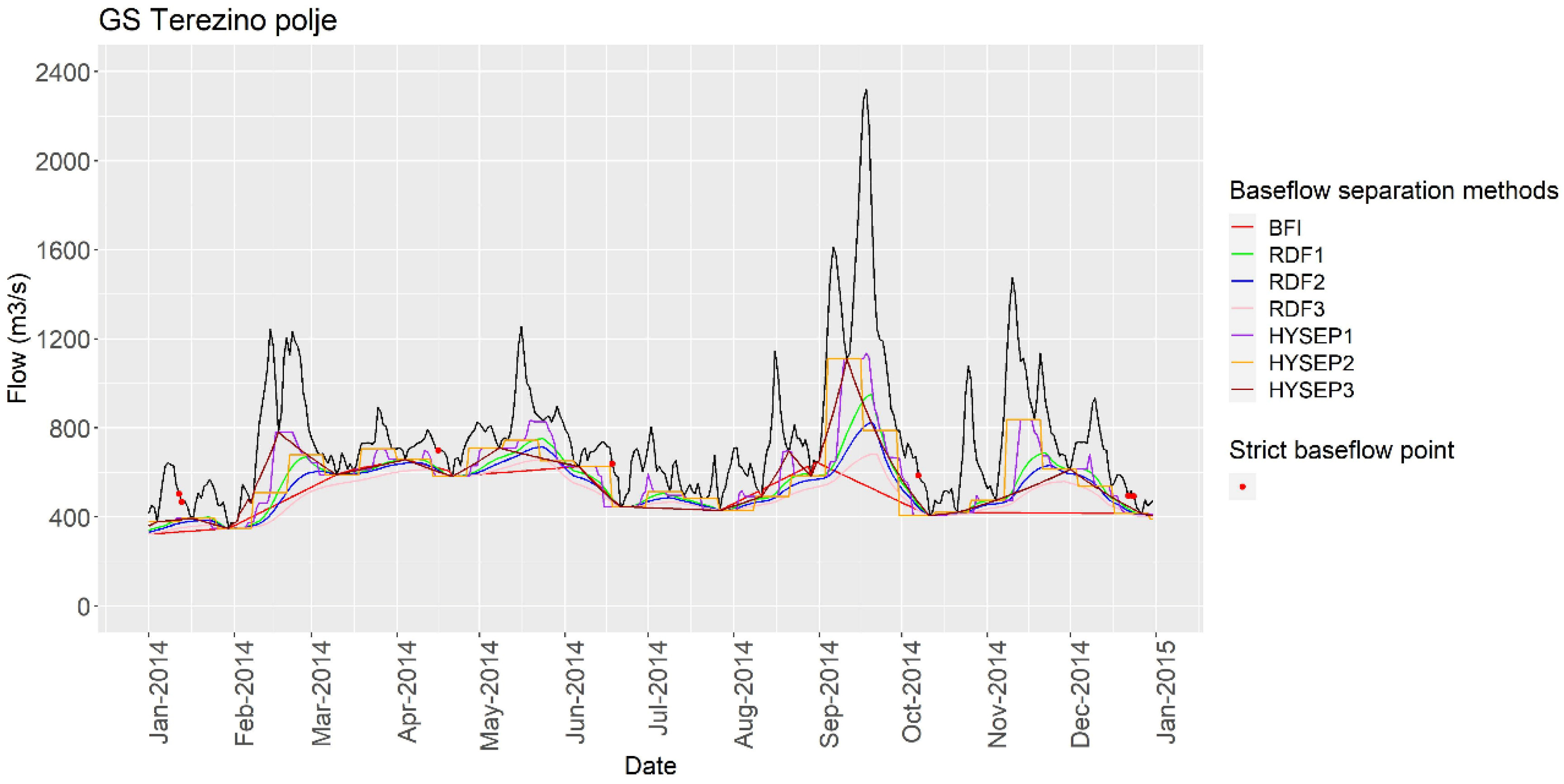
3.1. Selection of Baseflow Separation Method for Computing Flood Hydrograph Characteristics
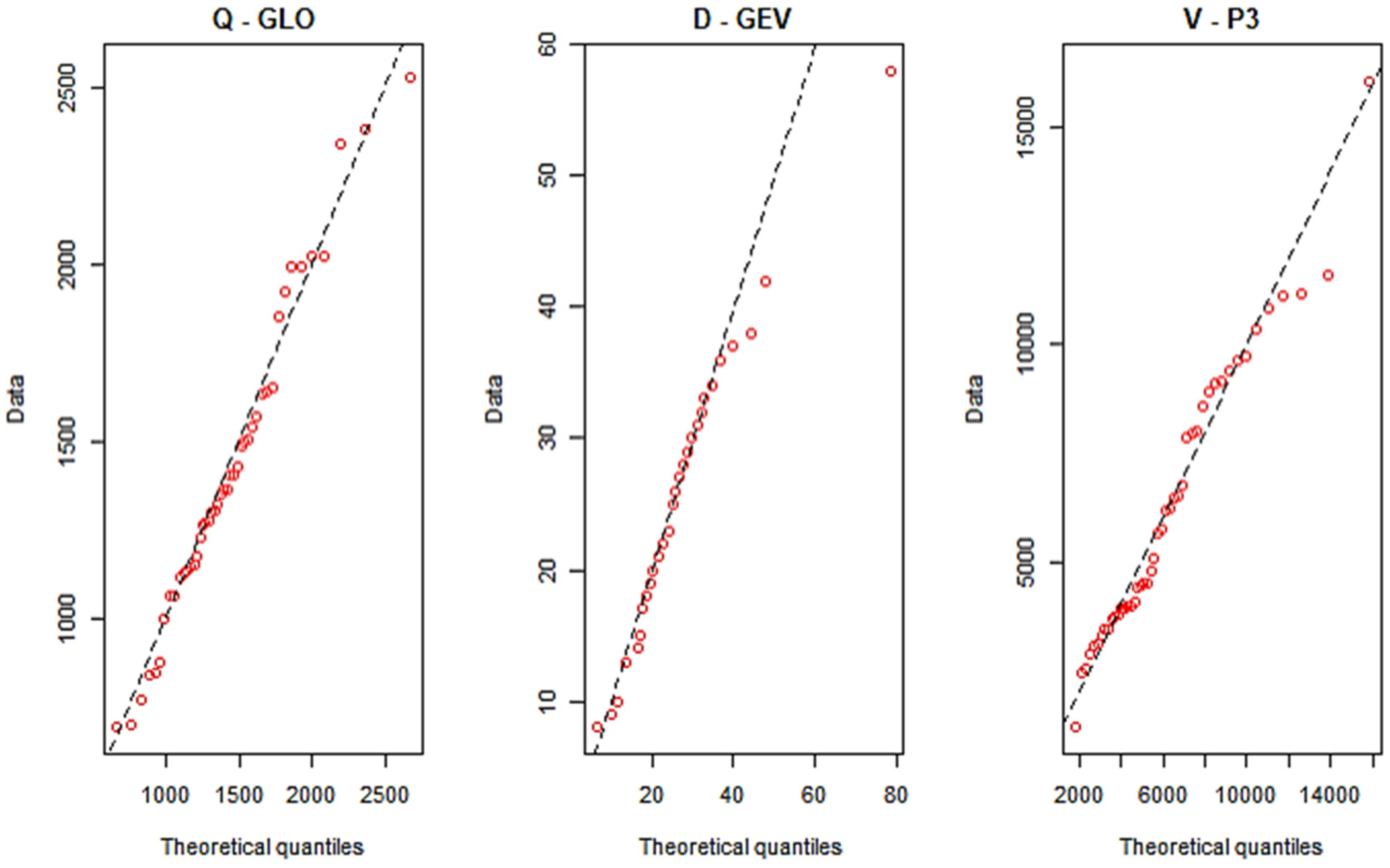
3.2. Selection of Marginal Probability Distributions for Q, D and V Series
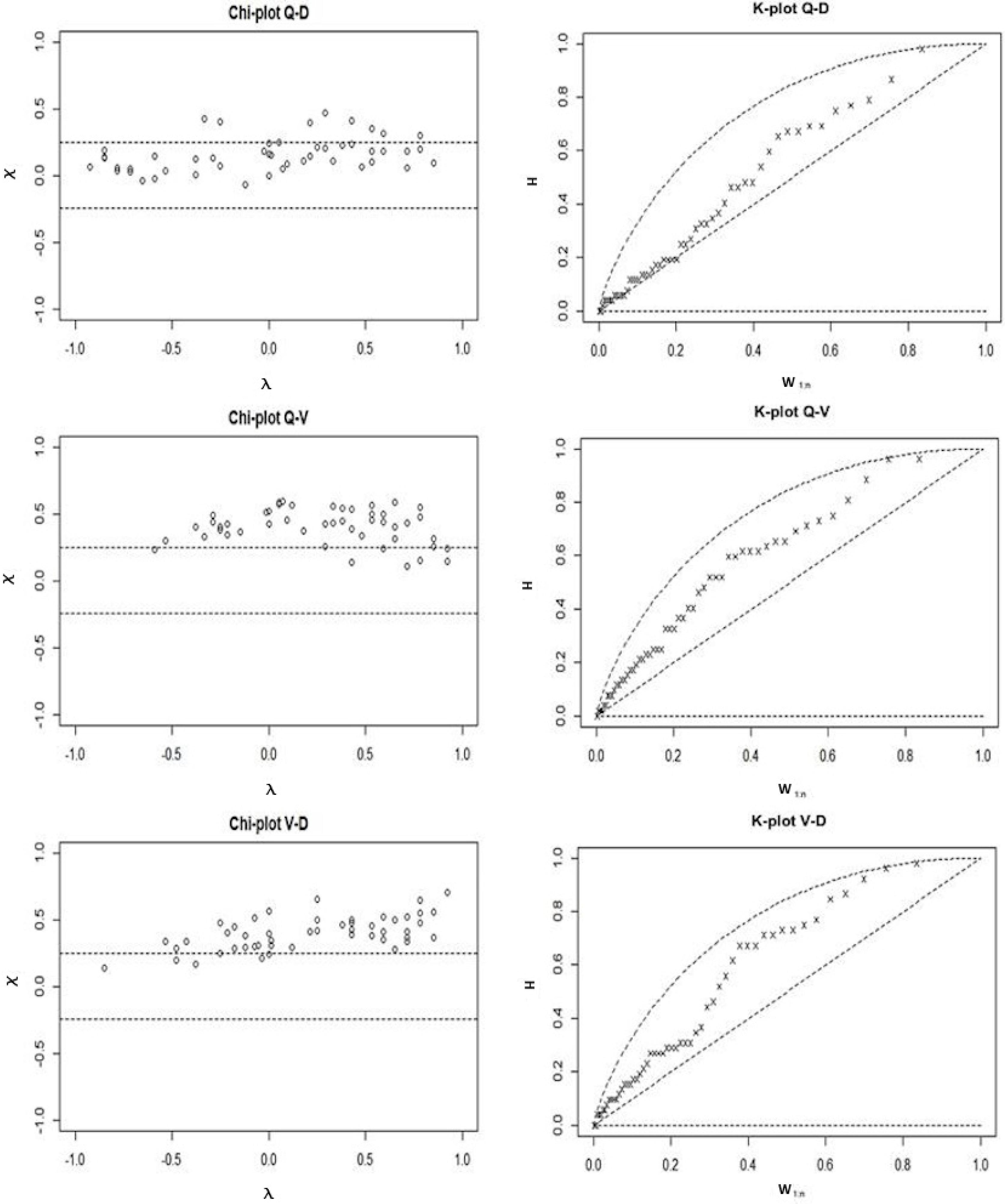
3.3. Copula Model Estimation
3.4. Joint Return Periods
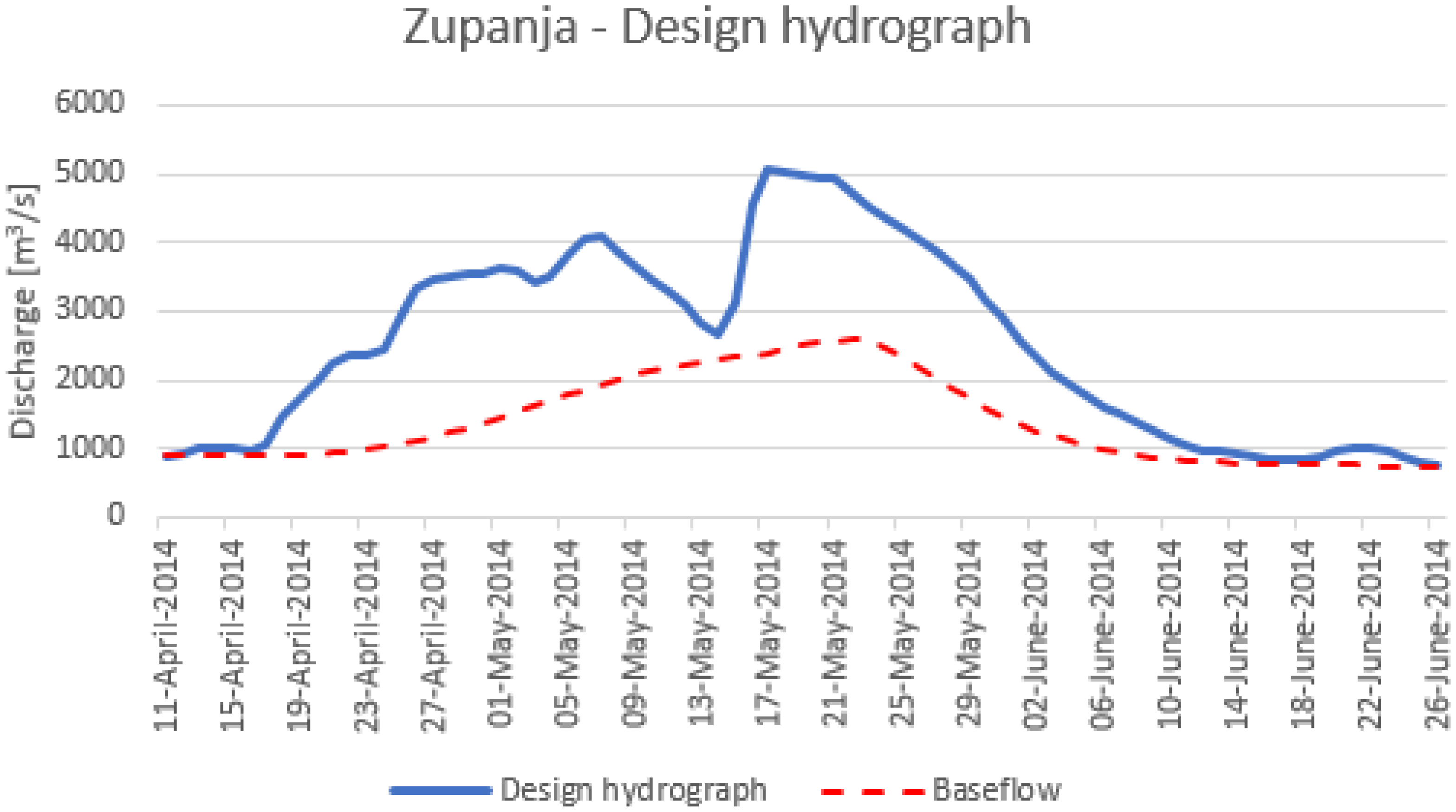
3.5. Preliminary Methodology for the Bridge Scour Analysis Using Copulas
4. Conclusions
- The HYSEP1 baseflow separation method can be regarded as an appropriate choice for baseflow separation for stations on the Drava River. In order to apply the baseflow evaluation criterion proposed by Xie et al. [59] at the stations in the middle part of the Sava River, additional analyses should be performed, or the proposed rules should be modified to correspond to the complex flood regime that prevails there. This indicates the importance of the visual inspection of the results, especially in the case of rivers where there are significant effects of dam operation and/or flood protection systems on flood hydrograph characteristics. Additionally, some of the tested baseflow separation methods did not yield useful results. Hence, it is advised that further studies that deal with flood hydrograph characteristics test multiple baseflow separation methods since extracted V and D variables can be highly sensitive to the selection of the baseflow separation methods. The differences among tested methods can yield V and D values that differ by an order of magnitude. Hence, this can lead to over- or under-estimation of the design variables.
- The Huesler–Reiss copula from the extreme-value family of copulas was selected as the most suitable copula for modelling peak discharges and hydrograph durations at all stations of the Drava River, while the most appropriate copula for modelling hydrograph volumes and hydrograph durations seems to be the Normal copula from the elliptical family of copulas. On the other hand, for the Sava River, more diverse results were obtained indicating non-uniform flow characteristics along the Sava River in Croatia.
- Different combinations of variables Q, D and V derived from the bivariate copula results for each station can eventually be computed if there is a need in practical applications (e.g., design, scour analysis, etc.). Hence, a preliminary methodology for the implication of the bivariate flood frequency analysis using copulas for the bridge scour analysis is proposed. As an example, the design hydrograph for one station on the Sava River is derived.
Author Contributions
Funding
Institutional Review Board Statement
Informed Consent Statement
Data Availability Statement
Acknowledgments
Conflicts of Interest
References
- Hung, C.-C.; Yau, W.-G. Behavior of scoured bridge piers subjected to flood-induced loads. Eng. Struct. 2014, 80, 241–250. [Google Scholar] [CrossRef]
- Ettema, R. Scour at Bridge Piers; Department of Civil Engineering, University of Auckland: Auckland, New Zeland, 1980; p. 527. [Google Scholar]
- Qadar, A. The Vortex Scour Mechanism At Bridge Piers. Proc. Inst. Civ. Eng. 1981, 71, 739–757. [Google Scholar] [CrossRef]
- Borghei, S.M.; Kabiri-Samani, A.; Banihashem, S.A. Influence of Unsteady Flow Hydrograph Shape on Local Scouring around Bridge Pier. In Proceedings of the Institution of Civil Engineers-Water Management; Thomas Telford Ltd.: London, UK, October 2012; Volume 165, pp. 473–480. [Google Scholar] [CrossRef]
- Imhof, D. Risk Assessment of Existing Bridge Structures; University of Cambridge: Cambridge, UK, 2004. [Google Scholar]
- Tosunoglu, F.; Gürbüz, F.; Ispirli, M.N. Multivariate modeling of flood characteristics using Vine copulas. Environ. Earth Sci. 2020, 79, 1–21. [Google Scholar] [CrossRef]
- Adamson, P.T.; Metcalfe, A.V.; Parmentier, B. Bivariate extreme value distributions: An application of the Gibbs Sampler to the analysis of floods. Water Resour. Res. 1999, 35, 2825–2832. [Google Scholar] [CrossRef]
- Han, C.; Liu, S.; Guo, Y.; Asce, M.; Lin, H.; Liang, Y.; Zhang, H. Copula-Based Analysis of Flood Peak Level and Duration: Two Case Studies in Taihu Basin, China. J. Hydrol. Eng. 2018, 23, 1661. [Google Scholar] [CrossRef]
- Zhang, L.; Singh, V.P. Bivariate Flood Frequency Analysis Using the Copula Method. J. Hydrol. Eng. 2006, 11, 150–164. [Google Scholar] [CrossRef]
- Latif, S.; Mustafa, F. Bivariate Hydrologic Risk Assessment of Flood Episodes using the Notation of Failure Probability. Civ. Eng. J. 2020, 6, 2002–2023. [Google Scholar] [CrossRef]
- Favre, A.-C.; El Adlouni, S.; Perreault, L.; Thiémonge, N.; Bobée, B. Multivariate hydrological frequency analysis using copulas. Water Resour. Res. 2004, 40, W01101. [Google Scholar] [CrossRef]
- Salvadori, G.; De Michele, C. Frequency analysis via copulas: Theoretical aspects and applications to hydrological events. Water Resour. Res. 2004, 40, 1–17. [Google Scholar] [CrossRef]
- Salvadori, G.; De Michele, C. Multivariate multiparameter extreme value models and return periods: A copula approach. Water Resour. Res. 2010, 46, W10501. [Google Scholar] [CrossRef]
- Genest, C.; Favre, A.-C. Everything You Always Wanted to Know about Copula Modeling but Were Afraid to Ask. J. Hydrol. Eng. 2007, 12, 347–368. [Google Scholar] [CrossRef]
- Reddy, M.J.; Ganguli, P. Bivariate Flood Frequency Analysis of Upper Godavari River Flows Using Archimedean Copulas. Water Resour. Manag. 2012, 26, 3995–4018. [Google Scholar] [CrossRef]
- Sraj, M.; Bezak, N.; Brilly, M. Bivariate flood frequency analysis using the copula function: A case study of the Litija station on the Sava River. Hydrol. Process. 2014, 29, 225–238. [Google Scholar] [CrossRef]
- Bezak, N.; Mikoš, M.; Šraj, M. Trivariate Frequency Analyses of Peak Discharge, Hydrograph Volume and Suspended Sediment Concentration Data Using Copulas. Water Resour. Manag. 2014, 28, 2195–2212. [Google Scholar] [CrossRef]
- Xing, Z.; Yan, D.; Zhang, C.; Wang, G.; Zhang, D. Spatial Characterization and Bivariate Frequency Analysis of Precipitation and Runoff in the Upper Huai River Basin, China. Water Resour. Manag. 2015, 29, 3291–3304. [Google Scholar] [CrossRef]
- Brunner, M.I.; Sikorska, A.E.; Seibert, J. Bivariate analysis of floods in climate impact assessments. Sci. Total Environ. 2017, 616–617, 1392–1403. [Google Scholar] [CrossRef]
- Li, T.; Wang, S.; Fu, B.; Feng, X. Frequency analyses of peak discharge and suspended sediment concentration in the United States. J. Soils Sediments 2019, 20, 1157–1168. [Google Scholar] [CrossRef]
- Li, Q.; Zeng, H.; Liu, P.; Li, Z.; Yu, W.; Zhou, H. Bivariate Nonstationary Extreme Flood Risk Estimation Using Mixture Distribution and Copula Function for the Longmen Reservoir, North China. Water 2022, 14, 604. [Google Scholar] [CrossRef]
- Hu, Y.; Liang, Z.; Huang, Y.; Yao, Y.; Wang, J.; Li, B. A nonstationary bivariate design flood estimation approach coupled with the most likely and expectation combination strategies. J. Hydrol. 2021, 605, 127325. [Google Scholar] [CrossRef]
- Naseri, K.; Hummel, M.A. A Bayesian copula-based nonstationary framework for compound flood risk assessment along US coastlines. J. Hydrol. 2022, 610, 128005. [Google Scholar] [CrossRef]
- Latif, S.; Simonovic, S.P. Parametric Vine Copula Framework in the Trivariate Probability Analysis of Compound Flooding Events. Water 2022, 14, 2214. [Google Scholar] [CrossRef]
- Sahoo, B.B.; Jha, R.; Singh, A.; Kumar, D. Bivariate low flow return period analysis in the Mahanadi River basin, India using copula. Int. J. River Basin Manag. 2019, 18, 107–116. [Google Scholar] [CrossRef]
- Wong, G.; Lambert, M.F.; Leonard, M.; Metcalfe, A.V. Drought Analysis Using Trivariate Copulas Conditional on Climatic States. J. Hydrol. Eng. 2010, 15, 129–141. [Google Scholar] [CrossRef]
- Liu, C.-L.; Zhang, Q.; Singh, V.P.; Cui, Y. Copula-based evaluations of drought variations in Guangdong, South China. Nat. Hazards 2011, 59, 1533–1546. [Google Scholar] [CrossRef]
- Ma, M.; Song, S.; Ren, L.; Jiang, S.; Song, J. Multivariate drought characteristics using trivariate Gaussian and Student t copulas. Hydrol. Process. 2011, 27, 1175–1190. [Google Scholar] [CrossRef]
- Brady, M.; Cong, R. Estimating the Resilience Value of Soil Biodiversity in Agriculture: A Stochastic Simulation Approach; LUND University: Lund, Swedish, 2011. [Google Scholar]
- De Michele, C. A Generalized Pareto intensity-duration model of storm rainfall exploiting 2-Copulas. J. Geophys. Res. Earth Surf. 2003, 108, 4067. [Google Scholar] [CrossRef]
- Tootoonchi, F.; Sadegh, M.; Haerter, J.O.; Räty, O.; Grabs, T.; Teutschbein, C. Copulas for hydroclimatic analysis: A practice-oriented overview. WIREs Water 2022, 9, e1579. [Google Scholar] [CrossRef]
- Peng, Y.; Shi, Y.; Yan, H.; Zhang, J. Multivariate Frequency Analysis of Annual Maxima Suspended Sediment Concentrations and Floods in the Jinsha River, China. J. Hydrol. Eng. 2020, 25, 05020029. [Google Scholar] [CrossRef]
- Plumb, B.D.; Juez, C.; Annable, W.K.; McKie, C.W.; Franca, M.J. The impact of hydrograph variability and frequency on sediment transport dynamics in a gravel-bed flume. Earth Surf. Process. Landf. 2019, 45, 816–830. [Google Scholar] [CrossRef]
- Harasti, A.; Gilja, G.; Potočki, K.; Lacko, M. Scour at Bridge Piers Protected by the Riprap Sloping Structure: A Review. Water 2021, 13, 3606. [Google Scholar] [CrossRef]
- Bezak, N.; Šraj, M.; Mikoš, M. Overview of Suspended Sediments Measurements in Slovenia and an Example of Data Analysis. Gradb. Vestn. 2013, 62, 274–280. [Google Scholar]
- Šraj, M.; Bezak, N.; Brilly, M. The Influence of the Choice of Method on the Results of Frequency Analysis of Peaks, Volumes and Durations of Flood Waves of The Sava River in Litija. Acta Hydrotech. 2012, 25, 41–58. [Google Scholar]
- Trninic, D. Hydrological Analysis of High Flows and Floods in the Sava River near Zagreb (Croatia). IAHS Publ.-Ser. Proc. Rep.-Int. Assoc. Hydrol. Sci. 1997, 239, 51–58. [Google Scholar]
- Gilja, G.; Ocvirk, E.; Kuspilić, N. Joint probability analysis of flood hazard at river confluences using bivariate copulas. Gradjevinar 2018, 70, 267–275. [Google Scholar] [CrossRef]
- Kovačević, M.; Potočki, K.; Gilja, G. The Analysis of Streamflow Variability and Flood Wave Characteristics on the Two Lowland Rivers in Croatia. In Proceedings of the EGU General Assembly Conference Abstracts, Online, 19–30 April 2021; p. EGU21-2563. [Google Scholar]
- Lacko, M.; Potočki, K.; Gilja, G. Determination of the Appropriate Baseflow Separation Method for Gauging Stations on the Two Lowland Rivers in Croatia. In Proceedings of the EGU General Assembly Conference Abstracts, Copernicus Meetings, Vienna, Austria, 23–27 May 2022; p. EGU22-7110. [Google Scholar]
- Tadić, L.; Bonacci, O.; Dadić, T. Analysis of the Drava and Danube rivers floods in Osijek (Croatia) and possibility of their coincidence. Environ. Earth Sci. 2016, 75, 1238. [Google Scholar] [CrossRef]
- Lóczy, D. The Drava River; Springer: Cham, Germany, 2019; pp. 61–90. [Google Scholar]
- Bonacci, O.; Oskoruš, D. The changes in the lower Drava River water level, discharge and suspended sediment regime. Environ. Earth Sci. 2009, 59, 1661–1670. [Google Scholar] [CrossRef]
- Pandžić, K.; Trninić, D.; Likso, T.; Bošnjak, T. Long-term variations in water balance components for Croatia. Arch. Meteorol. Geophys. Bioclimatol. Ser. B 2008, 95, 39–51. [Google Scholar] [CrossRef]
- Gajić-Čapka, M.; Cesarec, K. Trend and Variability in Discharge and Climate Variables in the Croatian Lower Drava River Basin. Hrvat. Vode 2010, 18, 19–30. [Google Scholar]
- Potočki, K.; Bekić, D.; Bonacci, O.; Kulić, T. Hydrological Aspects of Nature-Based Solutions in Flood Mitigation in the Danube River Basin in Croatia: Green vs. Grey Approach. In The Handbook of Environmental Chemistry; Springer: Berlin/Heidelberg, Germany, 2021. [Google Scholar]
- Anjevac, I.; OrešIć, D. Changes in Discharge Regimes of Rivers in Croatia. Acta Geogr. Slov. 2018, 58, 7–18. [Google Scholar]
- Bonacci, O.; Trninic, D. Hydrologische, Durch Die Aktivität Des Menschen Hervorgerufene Veränderungen Im Flussgebiet Der Save Bei Zagreb. Wasserwirtschaft 1991, 81, 171–175. [Google Scholar]
- Bonacci, O.; Ljubenkov, I. Procjena Sigurnosti Zagreba Od Poplava Vodama Rijeke Save u Novim Uvjetima. Hrvat. Vodoprivr. 2003, 12, 51–55. [Google Scholar]
- Bonacci, O.; Ljubenkov, I. Statistička Analiza Maksimalnih Godišnjih Protoka Save Kod Zagreba 1926–2000. Hrvat. Vode 2004, 48, 243–252. [Google Scholar]
- Bonacci, O.; Ljubenkov, I. Changes in flow conveyance and implication for flood protection, Sava River, Zagreb. Hydrol. Process. 2007, 22, 1189–1196. [Google Scholar] [CrossRef]
- Kratofil, L. Promjene Vodnog Režima Save Uzrokovane Ljudskom Djelatnošću. In Zbornik Radova Okruglog Stola “Hidrologija i Vodni Resursi Save u Novim Uvjetima”; Trninić, D., Ed.; Hrvatsko Hidrološko Društvo: Zagreb, Croatia, 2000; pp. 335–352. [Google Scholar]
- Šegota, T.; Filipčić, A. Suvremene promjene klime i smanjenje protoka Save u Zagrebu. Geoadria 2017, 12, 47–58. [Google Scholar] [CrossRef]
- Orešić, D.; Čanjevac, I.; Maradin, M. Changes in discharge regimes in the middle course of the Sava River in the 1931–2010 period. Pract. Geogr. 2017, 151, 93–119. [Google Scholar] [CrossRef]
- Sović, A.; Potočki, K.; Seršić, D.; Kuspilić, N. Wavelet Analysis of Hydrological Signals on an Example of the River Sava. In Proceedings of the 2012 35th International Convention MIPRO, Opatija, Croatia, 21–25 May 2012; pp. 1042–1047. [Google Scholar]
- Potočki, K.; Kuspilić, N.; Oskoruš, D. Wavelet Analysis of Monthly Discharge and Suspended Sediment Load on the River Sava. In Proceedings of the Thirteenth International Symposium on Water Management and Hydraulic Engineering-Proceedings, Slovak University of Technology, Bratislava, Slovakia, 9–12 September 2013; pp. 615–623. [Google Scholar]
- Lacko, M.; Potočki, K.; Pintar, D.; Humski, L.; Bojanjac, D. The Applicability of Functional Clustering in Analyzing Historical Floods of the Sava River in Zagreb. In Proceedings of the Abstract Book, Sixth International Workshop on Data Science; Lončarić, S., Šmuc, T., Eds.; Centre of Research Excellence for Data Science and Cooperative Systems Research Unit for Data Science: Zagreb, Croatia, 2021; pp. 67–69. [Google Scholar]
- Raffensperger, J.P.; Baker, A.C.; Blomquist, J.D.; Hopple, J.A. Optimal Hydrograph Separation Using a Recursive Digital Filter Constrained by Chemical Mass Balance, with Application to Selected Chesapeake Bay Watersheds; US Geological Survey: Reston, VA, USA, 2017; ISBN 141134135X. [Google Scholar]
- Xie, J.; Liu, X.; Wang, K.; Yang, T.; Liang, K.; Liu, C. Evaluation of typical methods for baseflow separation in the contiguous United States. J. Hydrol. 2020, 583, 124628. [Google Scholar] [CrossRef]
- Brutsaert, W. Long-term groundwater storage trends estimated from streamflow records: Climatic perspective. Water Resour. Res. 2008, 44, W02409. [Google Scholar] [CrossRef]
- Cheng, L.; Zhang, L.; Brutsaert, W. Automated Selection of Pure Base Flows from Regular Daily Streamflow Data: Objective Algorithm. J. Hydrol. Eng. 2016, 21, 06016008. [Google Scholar] [CrossRef]
- Gustard, A.; Bullock, A.; Dixon, J.M. Low Flow Estimation in the United Kingdom; Institute of Hydrology: Roorkee, India, 1992; ISBN 0948540451. [Google Scholar]
- Koffler, D.; Laaha, G. LFSTAT—An R-Package for Low-Flow Analysis. In Proceedings of the EGU General Assembly Conference Abstracts, Vienna, Austria, 22–27 April 2012; p. 8940. [Google Scholar]
- Lyne, V.; Hollick, M. Stochastic Time-Variable Rainfall-Runoff Modelling. In Proceedings of the Institute of Engineers Australia National Conference; Institute of Engineers Australia Barton: Sydney, Australia, 1979; Volume 79, pp. 89–93. [Google Scholar]
- Cuthbert, M.O. Straight thinking about groundwater recession. Water Resour. Res. 2014, 50, 2407–2424. [Google Scholar] [CrossRef]
- Hall, F.R. Base-Flow Recessions-A Review. Water Resour. Res. 1968, 4, 973–983. [Google Scholar] [CrossRef]
- Rutledge, A.T. Computer Programs for Describing the Recession of Ground-Water Discharge and for Estimating Mean Ground-Water Recharge and Discharge from Streamflow Records: Update; US Department of the Interior, US Geological Survey: Reston, VA, USA, 1998. [Google Scholar]
- Sujono, J.; Shikasho, S.; Hiramatsu, K. A comparison of techniques for hydrograph recession analysis. Hydrol. Process. 2004, 18, 403–413. [Google Scholar] [CrossRef]
- Nathan, R.J.; McMahon, T.A. Evaluation of automated techniques for base flow and recession analyses. Water Resour. Res. 1990, 26, 1465–1473. [Google Scholar] [CrossRef]
- Sloto, R.; Crouse, M. HYSEP—A Computer Program for Streamflow Hydrograph Separation and Analysis Hopewell Furnace National Historic Site View Project; Springer: Berlin/Heidelberg, Germany, 1996. [Google Scholar]
- Pettyjohn, W.A.; Henning, R.J. Preliminary Estimate of Regional Effective Ground-Water Recharge Rates in Ohio; Ohio State University, Water Resources Center: Columbus, OH, USA, 1979. [Google Scholar]
- Mann, H.B. Nonparametric Tests against Trend. Econom. J. Econom. Soc. 1945, 13, 245–259. [Google Scholar] [CrossRef]
- Kendall, M.G. Multivariate Analysis; Griffin London: London, UK, 1975; Volume 2. [Google Scholar]
- Ljung, G.M.; Box, G.E.P. On a Measure of Lack of Fit in Time Series Models. Biometrika 1978, 65, 297–303. [Google Scholar] [CrossRef]
- De Michele, C.; Salvadori, G.; Canossi, M.; Petaccia, A.; Rosso, R. Bivariate Statistical Approach to Check Adequacy of Dam Spillway. J. Hydrol. Eng. 2005, 10, 50–57. [Google Scholar] [CrossRef]
- Grimaldi, S.; Serinaldi, F. Asymmetric copula in multivariate flood frequency analysis. Adv. Water Resour. 2006, 29, 1155–1167. [Google Scholar] [CrossRef]
- Karmakar, S.; Simonovic, S. Bivariate flood frequency analysis: Part 1. Determination of marginals by parametric and nonparametric techniques. J. Flood Risk Manag. 2008, 1, 190–200. [Google Scholar] [CrossRef]
- Kar, K.K.; Yang, S.-K.; Lee, J.-H.; Khadim, F.K. Regional frequency analysis for consecutive hour rainfall using L-moments approach in Jeju Island, Korea. Geoenviron. Disasters 2017, 4, 18. [Google Scholar] [CrossRef]
- Zhang, L.; Singh, V.P. Bivariate rainfall frequency distributions using Archimedean copulas. J. Hydrol. 2007, 332, 93–109. [Google Scholar] [CrossRef]
- Chowdhary, H.; Escobar, L.A.; Singh, V.P. Identification of suitable copulas for bivariate frequency analysis of flood peak and flood volume data. Water Policy 2011, 42, 193–216. [Google Scholar] [CrossRef]
- Hosking, J.R.M.; Wallis, J.R. Regional Frequency Analysis; Cambridge University Press: Cambridge, UK, 1997; ISBN 0521430453. [Google Scholar]
- Bellosta, C.J.G.; Bellosta, M.C.J.G. Package ‘ADGofTest’. 2009. Available online: https://cran.r-project.org/web/packages/ADGofTest/index.html (accessed on 1 June 2022).
- Meylan, P.; Favre, A.-C.; Musy, A. Predictive Hydrology: A Frequency Analysis Approach; CRC Press: Boca Raton, FL, USA, 2012; ISBN 1578087473. [Google Scholar]
- Fisher, N.I.; Switzer, P. Chi-Plots for Assessing Dependence. Biometrika 1985, 72, 253–265. [Google Scholar] [CrossRef]
- I Fisher, N.; Switzer, P. Graphical Assessment of Dependence: Is a Picture Worth 100 Tests? Am. Stat. 2001, 55, 233–239. [Google Scholar] [CrossRef]
- Genest, C.; Boies, J.-C. Detecting Dependence With Kendall Plots. Am. Stat. 2003, 57, 275–284. [Google Scholar] [CrossRef]
- Morlot, M.; Brilly, M.; Šraj, M. Characterisation of the floods in the Danube River basin through flood frequency and seasonality analysis. Acta Hydrotech. 2019, 32, 73–89. [Google Scholar] [CrossRef]
- Nelsen, R.B. An Introduction to Copulas; Springer New York: New York, NY, USA, 1999; Volume 139, ISBN 978-0-387-98623-4. [Google Scholar]
- Kojadinovic, I.; Yan, J. Modeling Multivariate Distributions with Continuous Margins Using the Copula R Package. J. Stat. Softw. 2010, 34, 1–20. [Google Scholar] [CrossRef]
- Grønneberg, S.; Hjort, N.L. The Copula Information Criteria. Scand. J. Stat. 2014, 41, 436–459. [Google Scholar] [CrossRef]
- Bezak, N.; Rusjan, S.; Mikoš, M.; Šraj, M.; Fijavž, M.K. Estimation of Suspended Sediment Loads Using Copula Functions. Water 2017, 9, 628. [Google Scholar] [CrossRef]
- Salvadori, G.; de Michele, C.; Kottegoda, N.T.; Rosso, R. Extremes in Nature: An Approach Using Copulas; Springer Science & Business Media: Berlin/Heidelberg, Germany, 2007; Volume 56, ISBN 1402044151. [Google Scholar]
- Gräler, B.; Berg, M.J.V.D.; Vandenberghe, S.; Petroselli, A.; Grimaldi, S.; De Baets, B.; Verhoest, N.E.C. Multivariate return periods in hydrology: A critical and practical review focusing on synthetic design hydrograph estimation. Hydrol. Earth Syst. Sci. 2013, 17, 1281–1296. [Google Scholar] [CrossRef]
- Yue, S.; Rasmussen, P. Bivariate frequency analysis: Discussion of some useful concepts in hydrological application. Hydrol. Process. 2002, 16, 2881–2898. [Google Scholar] [CrossRef]
- Shiau, J.T. Return period of bivariate distributed extreme hydrological events. Stoch. Hydrol. Hydraul. 2003, 17, 42–57. [Google Scholar] [CrossRef]
- Tadić, L.; Brleković, T. Hydrological Characteristics of the Drava River in Croatia. In The Drava River; Springer: Berlin/Heidelberg, Germany, 2019; pp. 79–90. [Google Scholar]
- Yue, S.; Ouarda, T.B.M.J.; Bobée, B.; Legendre, P.; Bruneau, P. Approach for Describing Statistical Properties of Flood Hydrograph. J. Hydrol. Eng. 2002, 7, 147–153. [Google Scholar] [CrossRef]
- Brunner, M.I.; Viviroli, D.; Sikorska, A.E.; Vannier, O.; Favre, A.; Seibert, J. Flood type specific construction of synthetic design hydrographs. Water Resour. Res. 2017, 53, 1390–1406. [Google Scholar] [CrossRef]
- Bezak, N.; Matjaž, M.; Šraj, M. Razvoj Metodologije Za Določitev Projektnih Hidrogramov. In Proceedings of the Mišičev Vodarski Dan, Maribor, Slovenia, 2021. Available online: https://www.researchgate.net/publication/360155978_Razvoj_metodologije_za_dolocitev_projektnih_hidrogramov (accessed on 1 June 2022).
- Bezak, N.; Matjaž, M.; Lebar, K.; Šraj, M. Development of the Methodology for the Design Hydrograph Estimation in Slovenia, Europe. In Proceedings of the 39th IAHR World Congress, Granada, Spain, 19–24 June 2022; pp. 6877–6885. [Google Scholar] [CrossRef]


| River | Station | Watershed Area [km2] | Period; Years of Data | Qmax; Qmean; Qsd (m3/s) | Dmax; Dmean; Dsd (day) | Vmax; Vmean; Vsd (106 m3) |
|---|---|---|---|---|---|---|
| Drava | Botovo | 31,038.0 | 1962–2019; 47 | 2551; 1430; 464.6 | 58; 25; 10.3 | 1408; 558; 299.4 |
| Terezino polje | 33,916.0 | 1962–2019; 47 | 2778; 1379; 493.5 | 62; 26; 11.1 | 1511; 563; 315.8 | |
| Donji Miholjac | 37,142.0 | 1962–2019; 46 | 2140; 1269; 371.5 | 56; 27; 10.2 | 1367; 530; 282.3 | |
| Belisce | 38,500.0 | 1962–2019; 46 | 2035; 1242; 326.9 | 57; 25; 10.2 | 1355; 508; 273.0 | |
| Sava | Podsused | 12,316.0 | 1951–2019; 55 | 3038; 1648; 488.1 | 59; 25; 12.2 | 1195; 560; 221.7 |
| Jasenovac | 38,953.0 | 1951–2019; 53 | 2759; 1884; 371.1 | 113; 55; 20.8 | 4059; 1975; 850.5 | |
| Mackovac | 40,838.0 | 1951–2019; 53 | 3100; 1803; 393.7 | 129; 54; 23.4 | 5600; 2020; 1015.5 | |
| Zupanja | 62,891.0 | 1951–2019; 54 | 5317; 2679; 657.4 | 174; 63; 29.0 | 6274; 2956; 1326.5 |
| Copula Family | Copula | Cθ (u, v) |
|---|---|---|
| Archimedean | Gumbel–Hougaard | , θ ∈ [ 1, ∞) |
| Clayton | , θ ∈ [ −1, ∞) \ {0} | |
| Extreme value | Galambos | , θ ∈ [ 0, ∞) |
| Huesler–Reiss | , θ ∈ [ 0, ∞) | |
| Tawn | , θ ∈ [ 0;1] | |
| Elliptical | Normal | , θ ∈ [ −1;1] |
| River | Station | Evaluation Results | BFI | RDF1 | RDF2 | RDF3 | HYSEP1 | HYSEP2 | HYSEP3 |
|---|---|---|---|---|---|---|---|---|---|
| Drava | Botovo | NSE | −0.216 | 0.325 | 0.119 | −0.224 | 0.350 | 0.324 | 0.216 |
| Rank | 6 | 2 | 5 | 7 | 1 | 3 | 4 | ||
| Terezino polje | NSE | −0.189 | 0.337 | 0.118 | −0.248 | 0.407 | 0.367 | 0.238 | |
| Rank | 6 | 3 | 5 | 7 | 1 | 2 | 4 | ||
| Donji Miholjac | NSE | −0.109 | 0.361 | 0.149 | −0.207 | 0.440 | 0.413 | 0.237 | |
| Rank | 6 | 3 | 5 | 7 | 1 | 2 | 4 | ||
| Belisce | NSE | −0.277 | 0.266 | 0.023 | −0.378 | 0.387 | 0.313 | 0.164 | |
| Rank | 6 | 3 | 5 | 7 | 1 | 2 | 4 | ||
| Sava | Podsused | NSE | −0.003 | 0.444 | 0.290 | 0.039 | 0.530 | 0.525 | 0.264 |
| Rank | 7 | 3 | 4 | 6 | 1 | 2 | 5 | ||
| Jasenovac | NSE | 0.220 | 0.615 | 0.499 | 0.313 | 0.654 | 0.624 | 0.488 | |
| Rank | 7 | 3 | 4 | 6 | 1 | 2 | 5 | ||
| Mackovac | NSE | 0.188 | 0.627 | 0.507 | 0.315 | 0.678 | 0.650 | 0.480 | |
| Rank | 7 | 3 | 4 | 6 | 1 | 2 | 5 | ||
| Zupanja | NSE | 0.319 | 0.687 | 0.581 | 0.402 | 0.693 | 0.662 | 0.531 | |
| Rank | 7 | 2 | 4 | 6 | 1 | 3 | 5 |
| Year | Peak Date | Peak Value | Variable | BFI | RDF1 | RDF2 | RDF3 | HYSEP1 | HYSEP2 | HYSEP3 |
|---|---|---|---|---|---|---|---|---|---|---|
| 1962 | 6 June 1962 | 1367 | D (day) | 39 | 39 | 39 | 245 | 26 | 21 | 26 |
| V (106 m3) | 1327 | 1041 | 1192 | 4700 | 414 | 328 | 505 | |||
| 1963 | 15 March 1963 | 1683 | D (day) | 30 | 31 | 31 | 151 | 21 | 21 | 21 |
| V (106 m3) | 970 | 846 | 923 | 2533 | 684 | 789 | 807 | |||
| 1964 | 29 October 1964 | 1932 | D (day) | 40 | 69 | 69 | 69 | 25 | 23 | 25 |
| V (106 m3) | 1683 | 1618 | 1831 | 2132 | 788 | 842 | 875 | |||
| 1965 | 6 August 1965 | 2471 | D (day) | 29 | 29 | 29 | 37 | 29 | 22 | 29 |
| V (106 m3) | 1119 | 980 | 1020 | 1200 | 998 | 1001 | 1121 | |||
| 1966 | 23 August 1966 | 2525 | D (day) | 53 | 62 | 62 | 104 | 62 | 25 | 52 |
| V (106 m3) | 2047 | 1608 | 1763 | 2986 | 1404 | 1173 | 2086 | |||
| 1967 | 4 June 1967 | 1398 | D (day) | 24 | 50 | 50 | 161 | 9 | 9 | 9 |
| V (106 m3) | 486 | 933 | 1027 | 2678 | 267 | 205 | 248 | |||
| 1968 | 18 June 1968 | 811 | D (day) | 45 | 50 | 68 | 137 | 12 | 20 | 12 |
| V (106 m3) | 815 | 641 | 884 | 1958 | 161 | 221 | 160 | |||
| 1969 | 22 May 1969 | 979 | D (day) | 41 | 41 | 41 | 41 | 18 | 12 | 18 |
| V (106 m3) | 860 | 656 | 741 | 847 | 213 | 176 | 182 | |||
| 1970 | 14 August 1970 | 1390 | D (day) | 52 | 52 | 100 | 100 | 14 | 14 | 14 |
| V (106 m3) | 1228 | 855 | 1173 | 1367 | 353 | 324 | 354 | |||
| 1971 | 25 March 1971 | 717 | D (day) | 36 | 99 | 99 | 239 | 18 | 18 | 18 |
| V (106 m3) | 444 | 922 | 1058 | 2181 | 203 | 165 | 214 | |||
| 1972 | 19 July 1972 | 2882 | D (day) | 57 | 58 | 58 | 119 | 36 | 16 | 36 |
| V (106 m3) | 2415 | 1925 | 2093 | 2748 | 1511 | 978 | 2040 | |||
| 1973 | 30 September 1973 | 1749 | D (day) | 49 | 49 | 78 | 78 | 27 | 24 | 27 |
| V (106 m3) | 1729 | 1272 | 1635 | 1871 | 906 | 827 | 1085 | |||
| 1974 | 23 October 1974 | 1192 | D (day) | 47 | 29 | 61 | 61 | 15 | 15 | 15 |
| V (106 m3) | 1214 | 347 | 1030 | 1160 | 290 | 336 | 298 | |||
| 1975 | 5 July 1975 | 2578 | D (day) | 50 | 70 | 70 | 121 | 50 | 25 | 50 |
| V (106 m3) | 1932 | 1607 | 1776 | 2613 | 1174 | 879 | 1964 | |||
| 1976 | 29 April 1976 | 1108 | D (day) | 35 | 73 | 125 | 125 | 18 | 13 | 14 |
| V (106 m3) | 630 | 867 | 1380 | 1684 | 290 | 316 | 259 | |||
| 1977 | 11 April 1977 | 1137 | D (day) | 26 | 26 | 86 | 107 | 14 | 21 | 14 |
| V (106 m3) | 384 | 307 | 1193 | 1556 | 224 | 335 | 229 | |||
| 1978 | 14 June 1978 | 1226 | D (day) | 36 | 36 | 88 | 251 | 26 | 25 | 26 |
| V (106 m3) | 932 | 731 | 1535 | 3533 | 319 | 365 | 394 | |||
| 1979 | 22 November 1979 | 1428 | D (day) | 29 | 45 | 77 | 77 | 45 | 24 | 45 |
| V (106 m3) | 822 | 803 | 1121 | 1285 | 710 | 447 | 1028 | |||
| 1980 | 16 October 1980 | 1593 | D (day) | 27 | 30 | 70 | 112 | 30 | 21 | 30 |
| V (106 m3) | 1367 | 1248 | 1863 | 2562 | 1002 | 930 | 1439 | |||
| 1981 | 22 July 1981 | 1259 | D (day) | 49 | 50 | 67 | 67 | 29 | 22 | 29 |
| V (106 m3) | 822 | 645 | 762 | 840 | 502 | 517 | 632 | |||
| 1982 | 10 October 1982 | 1190 | D (day) | 40 | 48 | 48 | 48 | 24 | 21 | 24 |
| V (106 m3) | 1026 | 835 | 922 | 1025 | 520 | 589 | 632 | |||
| 1983 | 27 May 1983 | 862 | D (day) | 29 | 72 | 72 | 185 | 12 | 21 | 12 |
| V (106 m3) | 404 | 646 | 713 | 2046 | 142 | 164 | 140 | |||
| 1984 | 24 May 1984 | 1223 | D (day) | 41 | 41 | 94 | 94 | 21 | 22 | 21 |
| V (106 m3) | 995 | 777 | 1431 | 1713 | 296 | 421 | 290 | |||
| 1985 | 11 May 1985 | 1414 | D (day) | 45 | 45 | 45 | 83 | 16 | 22 | 12 |
| V (106 m3) | 1141 | 969 | 1119 | 1891 | 396 | 474 | 272 | |||
| 1986 | 19 June 1986 | 1370 | D (day) | 20 | 53 | 53 | 154 | 46 | 25 | 29 |
| V (106 m3) | 496 | 718 | 787 | 3564 | 661 | 492 | 672 | |||
| 1987 | 8 August 1987 | 1331 | D (day) | 31 | 31 | 31 | 66 | 21 | 12 | 21 |
| V (106 m3) | 659 | 572 | 616 | 1031 | 410 | 263 | 450 | |||
| 1988 | 9 June 1988 | 1058 | D (day) | 27 | 27 | 70 | 70 | 27 | 18 | 27 |
| V (106 m3) | 396 | 352 | 637 | 723 | 357 | 338 | 398 | |||
| 1989 | 8 July 1989 | 1772 | D (day) | 35 | 39 | 39 | 71 | 22 | 25 | 22 |
| V (106 m3) | 1174 | 1059 | 1147 | 1855 | 800 | 649 | 925 | |||
| 1990 | 4 November 1990 | 1321 | D (day) | 32 | 47 | 47 | 99 | 25 | 23 | 25 |
| V [(06 m3) | 712 | 747 | 800 | 1832 | 519 | 479 | 625 | |||
| 2003 | 4 November 2003 | 947 | D (day) | 28 | 28 | 36 | 91 | 16 | 16 | 16 |
| V (106 m3) | 401 | 389 | 450 | 1124 | 309 | 323 | 322 | |||
| 2004 | 28 June 2004 | 1155 | D (day) | 92 | 92 | 92 | 200 | 76 | 23 | 76 |
| V (106 m3) | 2551 | 1353 | 1553 | 3473 | 842 | 400 | 1998 | |||
| 2005 | 27 August 2005 | 1585 | D (day) | 36 | 36 | 36 | 36 | 36 | 24 | 36 |
| V (106 m3) | 1109 | 916 | 985 | 1062 | 772 | 574 | 1113 | |||
| 2006 | 2 June 2006 | 1185 | D (day) | 31 | 124 | 124 | 169 | 17 | 25 | 17 |
| V (106 m3) | 699 | 1802 | 2031 | 2868 | 287 | 385 | 231 | |||
| 2007 | 21 September 2007 | 749 | D (day) | 32 | 63 | 70 | 70 | 8 | 10 | 8 |
| V (106 m3) | 428 | 718 | 830 | 947 | 102 | 107 | 100 | |||
| 2008 | 9 June 2008 | 780 | D (day) | 78 | 85 | 139 | 139 | 26 | 20 | 26 |
| V (106 m3) | 1367 | 964 | 1437 | 1706 | 228 | 227 | 279 | |||
| 2009 | 29 June 2009 | 1129 | D (day) | 43 | 32 | 43 | 43 | 32 | 24 | 31 |
| V (106 m3) | 1240 | 706 | 982 | 1080 | 570 | 496 | 879 | |||
| 2010 | 22 September 2010 | 1634 | D (day) | 38 | 49 | 49 | 82 | 31 | 18 | 31 |
| V (106 m3) | 1095 | 937 | 1006 | 1585 | 762 | 639 | 994 | |||
| 2011 | 22 June 2011 | 789 | D (day) | 68 | 68 | 103 | 103 | 54 | 20 | 54 |
| V (106 m3) | 1182 | 773 | 1127 | 1323 | 590 | 337 | 990 | |||
| 2012 | 9 November 2012 | 1637 | D (day) | 82 | 82 | 82 | 116 | 31 | 25 | 30 |
| V (106 m3) | 2310 | 1393 | 1559 | 2380 | 770 | 736 | 1063 | |||
| 2013 | 11 May 2013 | 1313 | D (day) | 65 | 65 | 140 | 221 | 33 | 24 | 29 |
| V (106 m3) | 2021 | 1359 | 2222 | 3825 | 358 | 337 | 436 | |||
| 2014 | 18 September 2014 | 2322 | D (day) | 41 | 43 | 76 | 76 | 30 | 18 | 30 |
| V (106 m3) | 2209 | 1696 | 2459 | 2738 | 968 | 879 | 1114 | |||
| 2015 | 18 October 2015 | 1357 | D (day) | 35 | 35 | 35 | 105 | 35 | 25 | 35 |
| V (106 m3) | 1087 | 867 | 931 | 1415 | 755 | 579 | 1087 | |||
| 2016 | 4 May 2016 | 1045 | D (day) | 22 | 22 | 55 | 104 | 8 | 8 | 8 |
| V (106 m3) | 385 | 332 | 596 | 1464 | 197 | 176 | 160 | |||
| 2017 | 22 September 2017 | 1424 | D (day) | 39 | 44 | 44 | 44 | 44 | 25 | 44 |
| V (106 m3) | 874 | 761 | 818 | 879 | 671 | 655 | 984 | |||
| 2018 | 2 November 2018 | 1335 | D (day) | 46 | 63 | 63 | 86 | 30 | 24 | 30 |
| V (106 m3) | 1061 | 877 | 966 | 1169 | 631 | 640 | 834 | |||
| 2019 | 21 November 2019 | 1513 | D (day) | 45 | 51 | 51 | 51 | 43 | 25 | 37 |
| V (106 m3) | 1659 | 1284 | 1431 | 1624 | 896 | 572 | 1485 |
| River | Station | Mann–Kendall Test | Ljung–Box Test | ||||
|---|---|---|---|---|---|---|---|
| Variable | Test Statistic (S) | Z Value | p-Value | Test Statistic (Q) | p-Value | ||
| Drava | Botovo | Q | −44 | −0.394 | 0.693 | 0.417 | 0.518 |
| D | 143 | 1.304 | 0.192 | 0.297 | 0.586 | ||
| V | 65 | 0.587 | 0.557 | 0.893 | 0.345 | ||
| Terezino polje | Q | −121 | −1.101 | 0.271 | 1.292 | 0.256 | |
| D | −1 | 0.000 | 1.000 | 0.064 | 0.801 | ||
| V | −86 | −0.780 | 0.436 | 0.394 | 0.530 | ||
| Donji Miholjac | Q | −135 | −1.269 | 0.205 | 1.125 | 0.289 | |
| D | −137 | −1.290 | 0.197 | 0.508 | 0.476 | ||
| V | −117 | −1.098 | 0.272 | 0.322 | 0.571 | ||
| Belisce | Q | −221 | −2.083 | 0.037 | 2.053 | 0.152 | |
| D | −30 | −0.275 | 0.783 | 2.017 | 0.156 | ||
| V | −94 | −0.881 | 0.379 | 1.297 | 0.255 | ||
| Sava | Podsused | Q | 187 | 1.350 | 0.177 | 0.409 | 0.522 |
| D | 448 | 3.248 | 0.001 | 0.241 | 0.623 | ||
| V | 301 | 2.178 | 0.029 | 0.025 | 0.874 | ||
| Jasenovac | Q | 151 | 1.151 | 0.250 | 0.058 | 0.810 | |
| D | 144 | 1.098 | 0.272 | 0.861 | 0.354 | ||
| V | 122 | 0.928 | 0.353 | 1.157 | 0.282 | ||
| Mackovac | Q | 76 | 0.576 | 0.565 | 0.012 | 0.911 | |
| D | 85 | 0.645 | 0.519 | 0.041 | 0.840 | ||
| V | 34 | 0.253 | 0.800 | 0.004 | 0.949 | ||
| Zupanja | Q | −162 | −1.201 | 0.230 | 1.531 | 0.216 | |
| D | −28 | −0.202 | 0.840 | 1.168 | 0.280 | ||
| V | −115 | −0.851 | 0.395 | 0.043 | 0.837 | ||
| River | Station | Q | D | V |
|---|---|---|---|---|
| Drava | Botovo | GEV | GEV | Pearson 3 |
| Terezino polje | GLO | GEV | Pearson 3 | |
| Donji Miholjac | Pearson 3 | GLO | Pearson 3 | |
| Sava | Jasenovac | log-Pearson 3 | Pearson 3 | log-Pearson 3 |
| Mackovac | GLO | log-Pearson 3 | log-Pearson 3 | |
| Zupanja | GLO | GLO | log-Pearson 3 |
| River | Gauging Station | Sample Size | Q–D | Q–V | V–D |
|---|---|---|---|---|---|
| Drava | Botovo | 47 | 0.23 | 0.61 | 0.56 |
| Terezino polje | 47 | 0.36 | 0.72 | 0.56 | |
| Donji Miholjac | 46 | 0.27 | 0.70 | 0.44 | |
| Sava | Jasenovac | 53 | 0.21 | 0.49 | 0.47 |
| Mackovac | 54 | 0.15 | 0.36 | 0.56 | |
| Zupanja | 54 | 0.09 | 0.31 | 0.55 |
| River | Station | Q–D | Q–V | V–D | ||||||
|---|---|---|---|---|---|---|---|---|---|---|
| Copula | Sn | p-Value | Copula | Sn | p-Value | Copula | Sn | p-Value | ||
| Drava | Botovo | Huesler–Reiss | 0.038 | 0.937 | Huesler–Reiss | 0.033 | 0.078 | Normal | 0.023 | 0.471 |
| Terezino polje | Huesler–Reiss | 0.020 | 0.809 | Gumbel | 0.021 | 0.381 | Normal | 0.017 | 0.873 | |
| Donji Miholjac | Huesler–Reiss | 0.020 | 0.895 | Normal | 0.022 | 0.369 | Normal | 0.022 | 0.674 | |
| Sava | Jasenovac | Gumbel | 0.031 | 0.251 | Normal | 0.022 | 0.538 | Tawn | 0.033 | 0.413 |
| Mackovac | Tawn | 0.035 | 0.166 | Tawn | 0.020 | 0.873 | Gumbel | 0.035 | 0.052 | |
| Zupanja | Huesler–Reiss | 0.040 | 0.067 | Tawn | 0.043 | 0.055 | Normal | 0.018 | 0.793 | |
| Drava | Sava | |||||
|---|---|---|---|---|---|---|
| Return Period | Botovo | Terezino Polje | Donji Miholjac | Jasenovac | Mackovac | Zupanja |
| Q10 (m3/s) | 2054.7 | 1967.4 | 1778.1 | 2382.8 | 2278.8 | 3450.0 |
| Q10 (m3/s/km2) | 0.0662 | 0.0580 | 0.0479 | 0.0612 | 0.0558 | 0.0549 |
| D10 (day) | 38.7 | 40.8 | 39.4 | 83.2 | 86.4 | 98.9 |
| V10 (106 m3) | 970.2 | 999.3 | 920.9 | 3185.8 | 3366.2 | 4821.4 |
| V10 (m3/km2) | 31,258.3 | 29,464.3 | 24,793.0 | 81,786.2 | 82,429.3 | 76,662.3 |
| Q100 (m3/s) | 2910.9 | 3296.2 | 2411.4 | 2858.8 | 3199.2 | 5060.176 |
| Q100 (m3/s/km2) | 0.0938 | 0.0972 | 0.0649 | 0.0734 | 0.0783 | 0.0805 |
| D100 (day) | 51.5 | 59.9 | 58.5 | 111.6 | 127.5 | 157.0 |
| V100 (106 m3) | 1554.0 | 1674.2 | 1483.7 | 4554.1 | 5617.7 | 7451.7 |
| V100 (m3/km2) | 50,068.7 | 49,362.8 | 39,945.4 | 116,912.3 | 137,560.2 | 118,485.4 |
| Huesler–Reiss | Huesler–Reiss | Huesler–Reiss | Gumbel | Tawn | Huesler–Reiss | |
| TAND (Q10D10) | 30 | 22 | 26 | 28 | 36 | 51 |
| TOR (Q10D10) | 6 | 7 | 6 | 6 | 6 | 6 |
| TAND (Q100D100) | 364 | 238 | 303 | 329 | 462 | 835 |
| TOR (Q100D100) | 58 | 63 | 60 | 59 | 56 | 53 |
| TAND (Q10D100) | 148 | 114 | 131 | 151 | 226 | 271 |
| TOR (Q10D100) | 10 | 10 | 10 | 10 | 9 | 9 |
| TAND (Q100D10) | 148 | 114 | 131 | 151 | 226 | 271 |
| TOR (Q100D10) | 10 | 10 | 10 | 10 | 9 | 9 |
| Huesler–Reiss | Gumbel | Normal | Normal | Tawn | Tawn | |
| TAND (Q10V10) | 14 | 13 | 15 | 21 | 21 | 23 |
| TOR (Q10V10) | 8 | 8 | 8 | 7 | 7 | 6 |
| TAND (Q100V100) | 147 | 127 | 193 | 375 | 224 | 256 |
| TOR (Q100V100) | 76 | 82 | 68 | 58 | 64 | 62 |
| TAND (Q10V100) | 100 | 100 | 102 | 128 | 121 | 136 |
| TOR (Q10V100) | 10 | 10 | 10 | 10 | 10 | 10 |
| TAND (Q100V10) | 100 | 100 | 102 | 128 | 121 | 136 |
| TOR (Q100V10) | 10 | 10 | 10 | 10 | 10 | 10 |
| Normal | Normal | Normal | Tawn | Gumbel | Normal | |
| TAND (V10D10) | 20 | 19 | 24 | 19 | 15 | 19 |
| TOR (V10D10) | 7 | 7 | 6 | 7 | 7 | 7 |
| TAND (V100D100) | 316 | 312 | 479 | 199 | 156 | 306 |
| TOR (V100D100) | 59 | 60 | 56 | 67 | 74 | 60 |
| TAND (V10D100) | 118 | 117 | 145 | 109 | 102 | 116 |
| TOR (V10D100) | 10 | 10 | 10 | 10 | 10 | 10 |
| TAND (V100D10) | 118 | 117 | 145 | 109 | 102 | 116 |
| TOR (V100D10) | 10 | 10 | 10 | 10 | 10 | 10 |
Publisher’s Note: MDPI stays neutral with regard to jurisdictional claims in published maps and institutional affiliations. |
© 2022 by the authors. Licensee MDPI, Basel, Switzerland. This article is an open access article distributed under the terms and conditions of the Creative Commons Attribution (CC BY) license (https://creativecommons.org/licenses/by/4.0/).
Share and Cite
Lacko, M.; Potočki, K.; Škreb, K.A.; Bezak, N. Joint Modelling of Flood Hydrograph Peak, Volume and Duration Using Copulas—Case Study of Sava and Drava River in Croatia, Europe. Water 2022, 14, 2481. https://doi.org/10.3390/w14162481
Lacko M, Potočki K, Škreb KA, Bezak N. Joint Modelling of Flood Hydrograph Peak, Volume and Duration Using Copulas—Case Study of Sava and Drava River in Croatia, Europe. Water. 2022; 14(16):2481. https://doi.org/10.3390/w14162481
Chicago/Turabian StyleLacko, Martina, Kristina Potočki, Kristina Ana Škreb, and Nejc Bezak. 2022. "Joint Modelling of Flood Hydrograph Peak, Volume and Duration Using Copulas—Case Study of Sava and Drava River in Croatia, Europe" Water 14, no. 16: 2481. https://doi.org/10.3390/w14162481
APA StyleLacko, M., Potočki, K., Škreb, K. A., & Bezak, N. (2022). Joint Modelling of Flood Hydrograph Peak, Volume and Duration Using Copulas—Case Study of Sava and Drava River in Croatia, Europe. Water, 14(16), 2481. https://doi.org/10.3390/w14162481