Evaluation of TIGGE Precipitation Forecast and Its Applicability in Streamflow Predictions over a Mountain River Basin, China

Abstract

The number of numerical weather prediction (NWP) models is on the rise, and they are commonly used for ensemble precipitation forecast (EPF) and ensemble streamflow prediction (ESP). This study evaluated the reliabilities of two well-behaved NWP centers in the Observing System Research and Predictability Experiment (THORPEX) Interactive Grand Global Ensemble (TIGGE), the European Centre for Medium-Range Weather Forecasts (ECMWF) and the National Centers for Environmental Prediction (NCEP), in EPF and ESP over a mountain river basin in China. This evaluation was carried out based on both deterministic and probabilistic metrics at a daily temporal scale. The effectiveness of two postprocessing methods, the Generator-based Postprocessing (GPP) method, and the Bayesian Model Averaging (BMA) method were also investigated for EPF and ESP. Results showed that: (1) The ECMWF shows better performances than NCEP in both EPF and ESP in terms of evaluation indexes and representation of the hydrograph. (2) The GPP method performs better than BMA in improving both EPF and ESP performances, and the improvements are more significant for the NCEP with worse raw performances. (3) Both ECMWF and NCEP have good potential for both EPF and ESP. By using the GPP method, there are desirable EPF performances for both ECMWF and NCEP at all 7 lead days, as well as highly skillful ECMWF ESP for 1~5 lead days and average moderate skillful NCEP ESP for all 7 lead days. The results of this study can provide a reference for the applications of TIGGE over mountain river basins.

1. Introduction

The accurate and early forecast of river streamflow, as well as the possible uncertainties in it, have the prowess of providing critical information for water resource management and disaster mitigation [1,2,3]. Ground observations are the traditional sources of precipitation for hydrological applications, which can only provide short-term flood forecasts with a lead time of 1–24 h. Single-value deterministic precipitation forecasts provided by numerical weather prediction (NWP) centers are also popular for streamflow forecasting, which can provide extended flood warnings but lack uncertainty information. Building an Ensemble Streamflow Prediction (ESP) system by simulating a calibrated hydrological model using ensemble precipitation forecasts (EPFs) is one useful methodology to meet these requirements [4].

To accelerate the improvements in the accuracy of 1-day to 2-week high-impact weather forecasts, the Observing System Research and Predictability Experiment (THORPEX) project was proposed in 2003. The THORPEX Interactive Grand Global Ensemble (TIGGE) [5], a key component of THORPEX, has collected ensemble forecasts generated by more than 10 NWP centers around the world since 2006 [6]. Among them, the European Centre for Medium-Range Weather Forecasts (ECMWF) and National Centers for Environmental Prediction (NCEP) are more popular worldwide [7,8,9]. The successful applications of the TIGGE database before 2009 have been comprehensively reviewed by Cloke and Pappenberger [10]. Plenty of studies have evaluated ESP systems (ESPs) for flood forecasting and found that ESPs could provide desirable forecasts up to 10 lead day [4,11,12].

However, raw EPFs often contain systematic biases and spread deficiencies, as well as coarse spatial resolutions, which cannot directly drive hydrological models for ESPs [13,14,15]. Therefore, statistical postprocessing is a requisite to reduce biases and correct dispersion errors for raw EPFs [16]. To address this problem, various methods have been proposed, such as the Bayesian Model Averaging (BMA) [17], the Extended Logisitic Regression (ExLR) [18], and the Generated based Postprocessing method (GPP) [19], etc. Numerous studies have assessed the performances of different postprocessing methods from the point of view of either meteorology [20,21] or hydrology [9,22]. Schmeits and Kok [23] compared the raw ECMWF ensemble forecasts and forecasts postprocessed with either a modified BMA method or the ExLR method in the Netherlands. The results showed that both the modified BMA and the ExLR could improve the raw ECMWF ensemble forecasts significantly for the first 5 forecast days. Li, Jiang [24] applied the postprocessed precipitation forecast to drive a calibrated hydrological model to predict ensemble streamflow. They found that both the forecast reliability and sharpness of ensemble streamflow forecasts showed improvements. Zhang, Chen [25] evaluated NCEP ensemble forecasts corrected by GPP in a southern basin of China and found that the corrected NCEP could provide desirable forecasts up to 9 and 5 lead days for precipitation and flood season streamflow, respectively.

Although there are lots of studies concentrating on precipitation forecasts [26,27] and streamflow predictions [10,28] for TIGGE and the effectiveness of postprocessing methods [5,29,30], few studies explore both the performances of TIGGE ensemble precipitation forecasts and their applicability in streamflow predictions over mountain river basins. Qi, Zhi [27] investigated the performances of the raw and postprocessed ensemble forecasts of heavy precipitation in mountainous areas, while they did not investigate their performances in ensemble streamflow prediction. This study aims to evaluate raw and postprocessed EPFs and assess the degree of improvement with different postprocessing methods to verify the reliabilities of EPF and ESP in a western mountain basin of China. Two well-behaved NWP centers in the TIGGE archive, i.e., ECMWF and NCEP, were evaluated in this study. Two popular postprocessing methods, i.e., GPP and BMA, were used to postprocess EPFs. Both deterministic and probabilistic metrics were used for the evaluation. Specifically, the objectives of this study are to answer the following two questions: (1) How do the ECMWF and NCEP perform in precipitation forecasting and streamflow prediction over a mountain river basin? (2) How do the two postprocessing methods, GPP and BMA, perform in improving the skill of EPF and ESP?

2. Study Area and Datasets

The Qingjiang River Basin (108°35′–111°35′ E, 22°33′–30°50′ N), a tributary of the Yangtze River, is located in southwestern Hubei Province in south-central China. It has an approximate total drainage area of 16,700 km² and a stream length of 423 km. This work focuses on the upper Qingjiang River basin (Figure 1), which is dominated by mountains and hills. The study area is dominated by a humid subtropical monsoon climate with four clear seasons. The annual average temperature is 14.1 °C, the coldest month is January, and the warmest month is generally July. The precipitation shows a significant time variation, with an annual average precipitation of approximately 1400 mm that is mostly concentrated in the flood season (April–September). The flow regime of the Qingjiang River is characterized by a seasonally fluctuating flow due to rainstorms in the rainy season [31]. Figure 1 shows the location of the Qingjiang River basin and the distribution of hydrological and meteorological stations.

In this study, both observations and EPFs at the daily time step were used. The observations include daily air temperature, precipitation, and potential evaporation, as well as streamflow from 2014 to 2017. The meteorological data were obtained from 175 automatic weather stations, and hydrological data were obtained from the Shuibuya hydropower station (Figure 1). The ensemble precipitation forecasts used in this study were obtained from two well-behaved NWP centers in the TIGGE database, i.e., ECMWF and NCEP. Information of the models, including model sources, forecast length, number of ensembles, and initial date of TIGGE operational model, is shown in

Table 1. The ensemble precipitation forecasts.

Center	Country/Region	Ensemble Members (Perturbed)	Base Time	Spatial Resolution	Forecast Length
ECMWF	Europe	50	00 UTC	0.5° × 0.5°	360 h at 6 h
NCEP	America	20	00 UTC	0.5° × 0.5°	384 h at 6 h

. The precipitation forecasts with a spatial resolution of 0.5° × 0.5° at 1–~7 lead days from 2014 to 2017 were evaluated in this study.

3. Methodology

3.1. Postprocessing Methods

A generator-based method, the GPP, and a distribution-based method, the BMA, which have been widely used and proven to be beneficial [9,23,32], were used to postprocess ensemble precipitation forecasts in this study. The parametric probability distribution function (PDF) denoted by g for the precipitation is as follows [32]:

$$y|x_1,\dots ,x_M~g(y|x_1,\dots ,x_k)$$

(1)

where y and x₁,…, x_k represent the variable of precipitation and the ensemble precipitation forecasts with K members, respectively. The PDF of precipitation is characterized by a mixed discrete/continuous distribution: a positive probability of being exactly zero, and a continuous skewed distribution for positive precipitation amounts. A mixed distribution model for precipitation proposed by Sloughter, Raftery [33] is as follows:

$$g(y|f_k)=P(y=0|f_k)\cdot I(y=0)+P(y>0|f_k)\cdot g_k(y|f_k)\cdot I(y>0)$$

(2)

where given the member forecast $f_k$,$g(y|f_k)$ represents the probability distribution, and I(…) represents unity if the condition in brackets holds, and zero otherwise; $P(y=0|f_k)$ and $g(y>0|f_k)$ represent the probabilities of non-precipitation and precipitation above zero, respectively. $g_k(y|f_k)$ represents a two-parameter gamma distribution. Different postprocessing methods differ in the ways of calibrating the PDF for precipitation and generating the postprocessed ensemble precipitation forecasts.

For GPP [19], the PDF of the precipitation in different seasons or magnitudes is calibrated independently to fit the observations. Then, the postprocessed EPFs are accordingly resampled from the calibrated PDF based on the forecast information within raw EPFs. For BMA [17], the PDF of the precipitation at different days or periods is calibrated to fit the ensemble forecasts according to a historical training set, including both EPFs and observations, as follows:

$$P(y|f_1,\dots ,f_k)=\frac{1}{K_{\sigma }}{\displaystyle \sum _{k=1}^{K}N(\frac{y-z_k}{\sigma })}$$

(3)

where N(…) represents the normal distribution with the mean $z_k$ and difference σ of the ensemble forecasts.

In this study, given the 4-year (2014–2017) available EPFs and observations, the postprocessing was conducted by using the cross-validation method. Specifically, when generating forecasts for a particular year, the remaining 3-year forecasts were used as the training data to calibrate the postprocessing method. The ensemble size of the postprocessed EPFs was set to 1000 to better represent the calibrated PDF. The postprocessing was conducted by using the MATLAB software.

3.2. Hydrological Model

The Xin’anjiang (XAJ) [34], a conceptual rainfall–runoff model, was adopted for hydrological simulation and forecasting in this study. The XAJ model is easy to use with minimum input data preparation, which has been widely used worldwide [25,28,35]. Figure 2 shows the flowchart of the XAJ model. There are four parts of calculation process within the XAJ [35]: (1) The evaporation module, which calculates the evaporation in three soil layers, including an upper layer, a lower layer, and a deep layer, based on the watershed saturation–excess runoff theory. (2) The runoff yielding module, which uses the storage curve to calculate the total runoff based on the concept of runoff formation on repletion of storage. Therefore, the runoff is not generated until soil moisture reaches the filled capacity. (3) The runoff sources partition module, which divides the total runoff into three components (surface runoff, interflow, and groundwater runoff) by using a free water capacity distribution curve. (4) Finally, the runoff concentration module, in which the surface runoff is routed by the unit hydrograph, and the interflow and groundwater flow are routed by the linear reservoir method. A total of 15 parameters need to be calibrated within the XAJ model: four related to evaporation, two related to runoff generation, and nine related to runoff routing. More details can be found in Ren-Jun [34].

The XAJ model needs basin-averaged precipitation, temperature, and potential evaporation as inputs, which were calculated by using the Thiessen Polygon method based on the collected datasets in this study. It was calibrated during the 2014–2016 period and validated during the 2017 period. During the calibration, the SCE-UA algorithm [36] was used to optimize model parameter sets based on the well-known objective functions of the Nash and Sutcliffe efficiency (NSE) [37] and water volume Relative Error (RE). The NSE and RE are defined as follows:

$$NSE=1-\frac{{\displaystyle \sum _{i=1}^n(Q_i^{obs}-Q_i^{sim})}}{{\displaystyle \sum _{i=1}^n(Q_i^{obs}-\overline{Q_i^{obs}})}}$$

(4)

$$RE(\%)=\frac{{\displaystyle \sum _{i=1}^n(Q_i^{obs}-Q_i^{sim})}}{{\displaystyle \sum _{i=1}^n(Q_i^{obs})}}\times 100$$

(5)

where $Q_i^{obs}$ represents the daily observed streamflow on the ith day, and $Q_i^{sim}$ represents the simulated value. ${\overline{Q}}^{obs}$ represents the average value of all the daily observed streamflow. The NSE ranges from minus infinity to 1 and the RE ranges from 0 to infinity. A larger NSE and a smaller RE represent a better performance.

3.3. Verification Metrics

In this study, both deterministic and probabilistic metrics were adopted from the Ensemble Verification System [38] to evaluate the performance of EPFs and ESPs. The Mean Absolute Error (MAE) and Continuous Ranked Probability Skill Score (CRPSS) were selected to assess deterministic and probabilistic performances, respectively.

(1) The MAE was used to measure the mean absolute difference of the ensemble mean forecasts and the observations as follows:

$$MAE=\frac{1}{N}{\displaystyle \sum _{t=1}^N\left|F_i-O_i\right|}$$

(6)

where $F_i$ and $O_i$ represent the forecasts and observations, respectively. The MAE ranges from 0 to infinity, and a smaller MAE indicates a better performance.

(2) The CRPSS was used to verify the ensemble information when computing the forecast skill. It is calculated based on the Continuous Ranked Probability Score (CRPS), which quantifies the mean squared difference between the distribution of ensemble forecasts and corresponding distributions of observations. The CRPS and CRPSS are defined as follows:

$$CRPS={\displaystyle \underset{-\infty }{\overset{+\infty }{\int }}{\left(P_F(x)-Po(x)\right)}^2}dx$$

(7)

$$CRPSS=1-\frac{CRPS}{CRP{S}^{*}}$$

(8)

where $P_F$, $P_O$, and x represent the cumulative distribution functions (CDFs) of the forecasts and observations, and the event to be analyzed, respectively. CRPS* represents the value of the reference forecasts [39]. The CRPSS ranges from minus infinity to 1, and a larger CRPSS indicates a better performance.

Another popular diagnostic tool in forecast verification, the relative operating characteristic (ROC) curve was used to assess the forecast’s ability [40]. The ROC curve plots the hit rate (HR) versus the false alarm rate (FAR) of a precipitation event for incremental decision thresholds. The closer the ROC curve to the upper left corner of the diagram (low false alarms, high hits), the greater the ability of discriminating precipitation events it reflects [41].

4. Results and Discussion

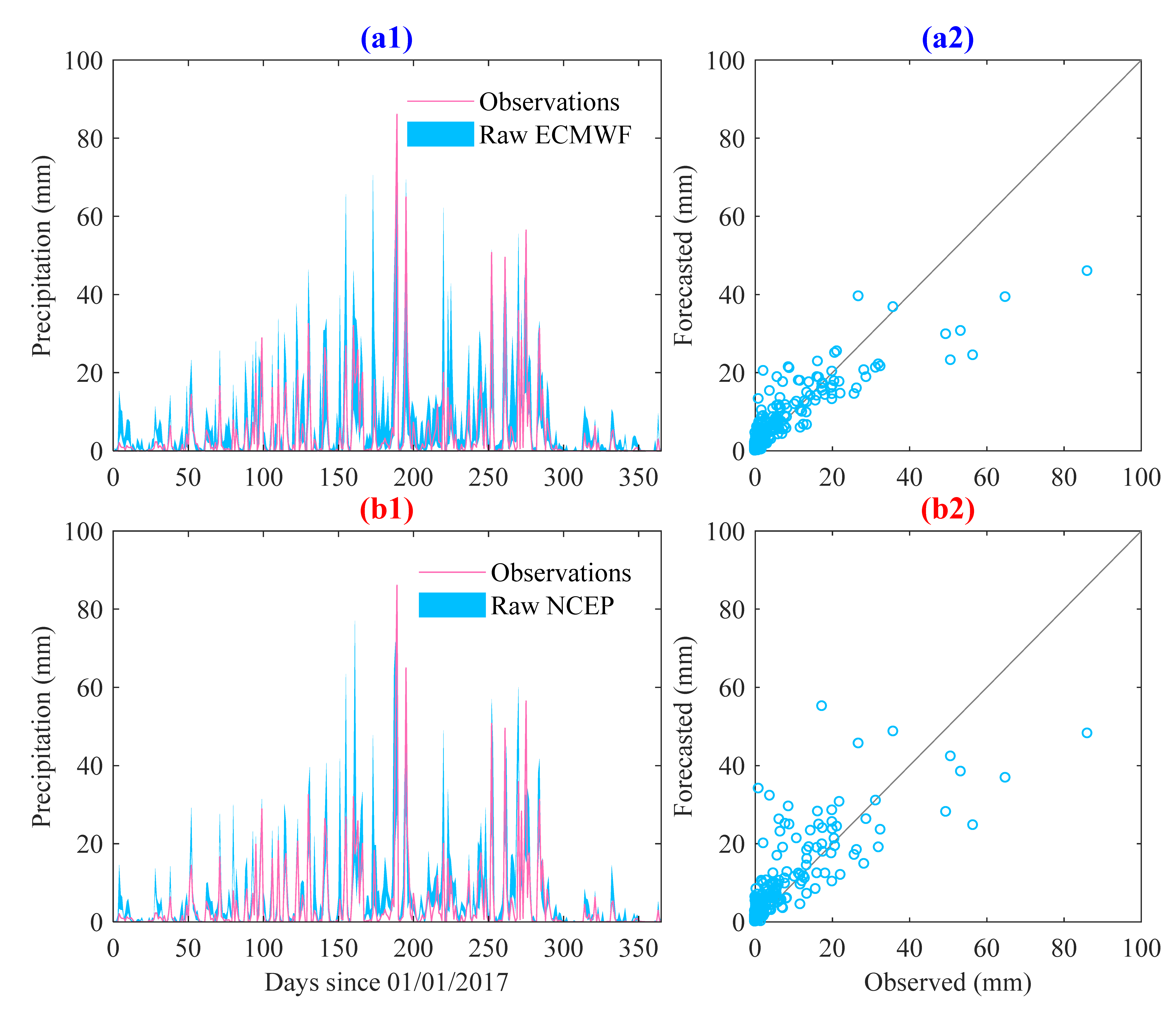
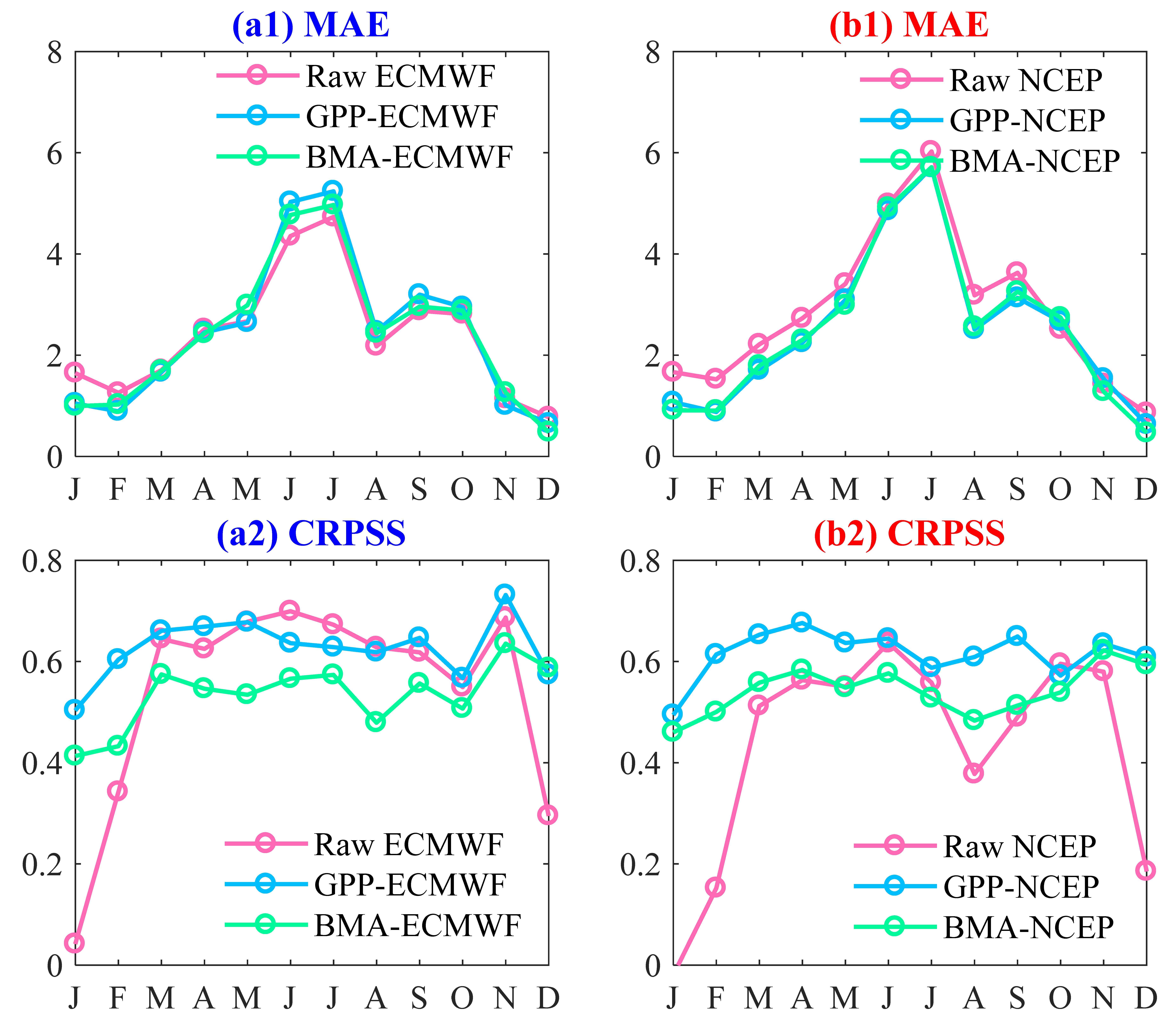
4.1. Performance of the Ensemble Precipitation Forecasts

Figure 3 presents the comparison of daily observed precipitation and raw EPFs from ECMWF (a1–a2) and NCEP (b1–b2) at 1 lead day during 2017. The left subplots are the time series of forecast and observed precipitation, and the right subplots are the scatter plots of ensemble mean forecast and observed precipitation. The time series of forecast and observed precipitation show that there are substantial biases between raw EPFs and observations. The scatter plots show significant underestimations of peak events by raw EPFs from both ECMWF and NCEP, which is consistent with the findings of previous studies [25,42,43]. Liu, Sun [42] found that heavy precipitation was generally underestimated over all of China, especially in the western region of China and South China due to the resolution and the related parameterization of convection. The underestimation of heavy precipitation is a concern of hydrological forecasting centers predicting discharge peaks and timing, as indicated by Jha, Shrestha [44].

Figure 4 presents the MAE and CRPSS of raw and postprocessed EPFs at all 7 lead days. Figure 4(a1,a2) are for ECMWF, and (b1–b2) are for NCEP. It can be seen that: (1) The MAE of raw ECMWF and NCEP are about 2.40~3.92 and 2.86~6.20 at all 7 lead days, respectively. The CRPSS of raw ECMWF and NCEP are about 0.49~0.65, 0.12~0.56 at all 7 lead days, respectively. The smaller MAE and larger CRPSS of ECMWF reveal better performance than NCEP. (2) The MAE/CRPSS values of the ensemble precipitation forecasts show a clear increase/decrease with the increase in the lead days, indicating a significant downward trend of the performance. (3) Figure 4(a1,a2) show that there are no significant improvements for ECMWF after postprocessing in terms of MAE and CRPSS. The CRPSS value of BMA-ECMWF is even slightly smaller than that of raw ECMWF. (4) Figure 4(b1,b2) show that both two postprocessing methods gain in skill compared to raw NCEP. Specifically, the MAE of GPP-NCEP decreases by 0.35~1.94 mm for 1~7 lead days; the MAE of BMA-NCEP decreases by 0.36~2.02 mm for 1~7 lead days. The CRPSS of GPP-NCEP increases by 0.09~0.34 for 1~7 lead days; the CRPSS of BMA-NCEP increases by 0.02~0.31 for 1~7 lead days. Moreover, the MAE and CRPSS ranges of postprocessed EPFs are both narrower than those of raw EPFs. These positive effects of the postprocessing methods for raw NCEP proved its necessity. Generally, the results above demonstrate that the GPP method performs better than the BMA method in improving forecasting skill and indicate the effectiveness of the postprocessing method for NCEP with a relatively inferior raw performance.

Figure 5 presents the monthly variation in MAE and CRPSS of raw and postprocessed EPFs at 1 lead day. Figure 5(a1,b1) show evident monthly variation in MAE of both raw and postprocessed EPFs, where there are larger values in June–July and smaller values in winter. There is little difference in MAE values between postprocessed and raw EPFs. Figure 5(a2,b2) also show evident monthly variation in CRPSS for raw EPFs, where the values in winter are much larger than those in other months, and the difference is up to 0.6, while the monthly variation in CRPSS for postprocessed EPFs are no longer larger, which is less than 0.23 and 0.18 for ECMWF and NCEP, respectively.

To further assess the forecast’s ability to discriminate heavy rain events, the ROC curves for 50 mm/day rainfall thresholds, at 1, 3, 5, and 7 lead days for raw and postprocessed ECMWF (solid line) and NCEP (dash line) are shown in Figure 6. The figure shows forecast discrimination of ECMWF is stronger than that of NCEP, where solid lines are closer to left corner of the plot than dash lines. For raw- and GPP-EPFs (Figure 6a,b), the ROC curves at 1, 3, 5, and 7 lead days increasingly move away from the top left corner of the plot, indicating that forecasts for shorter lead times have higher discriminative ability than those for longer lead times. This is not the case for BMA-EPFs (Figure 6c) with ROC curves for 7 lead days closer to the top left corner. Compared to the raw EPFs, GPP-EPFs demonstrate better forecasting ability in discriminating heavy rain events, while the opposite is true for BMA-EPFs.

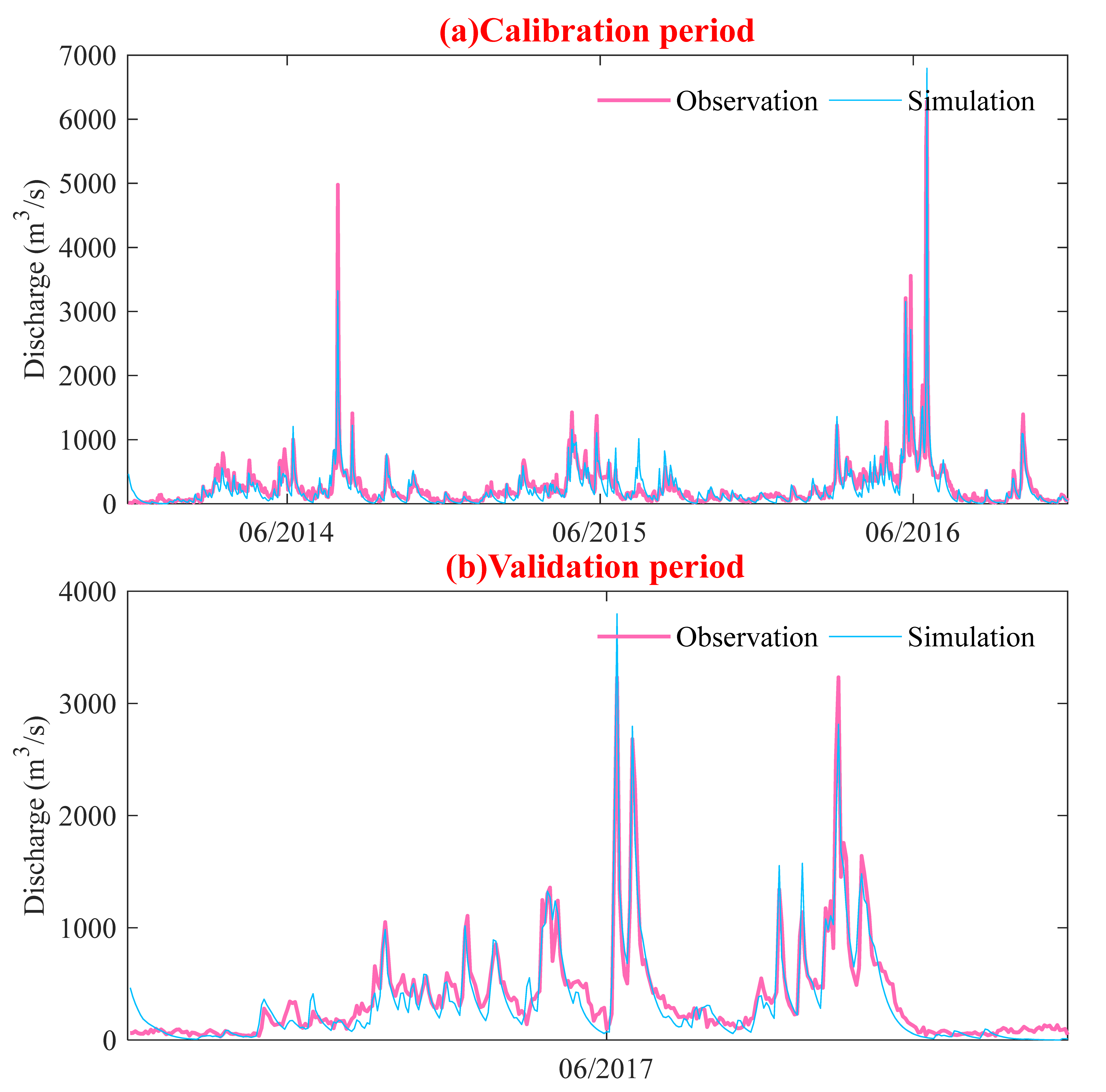
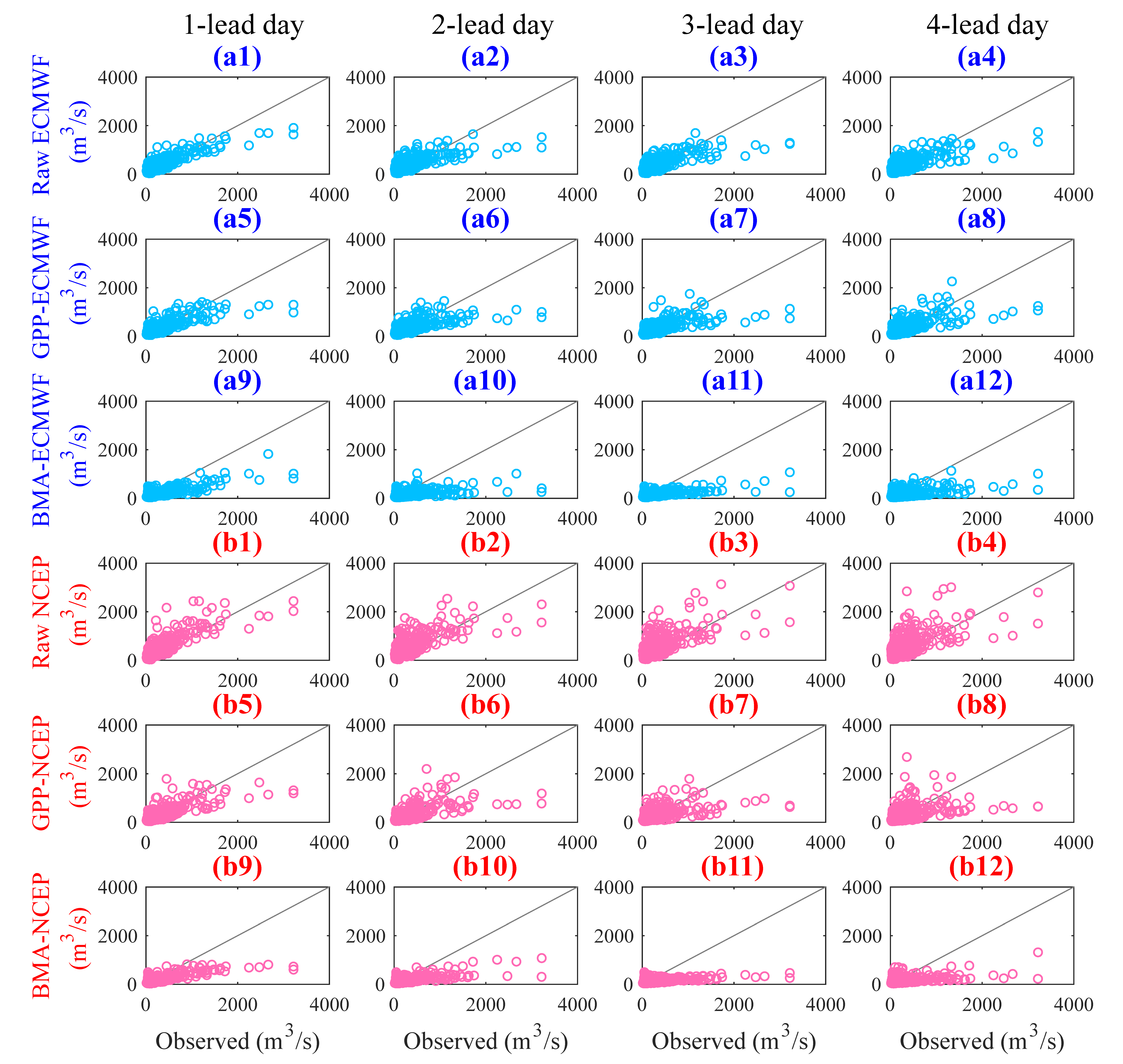
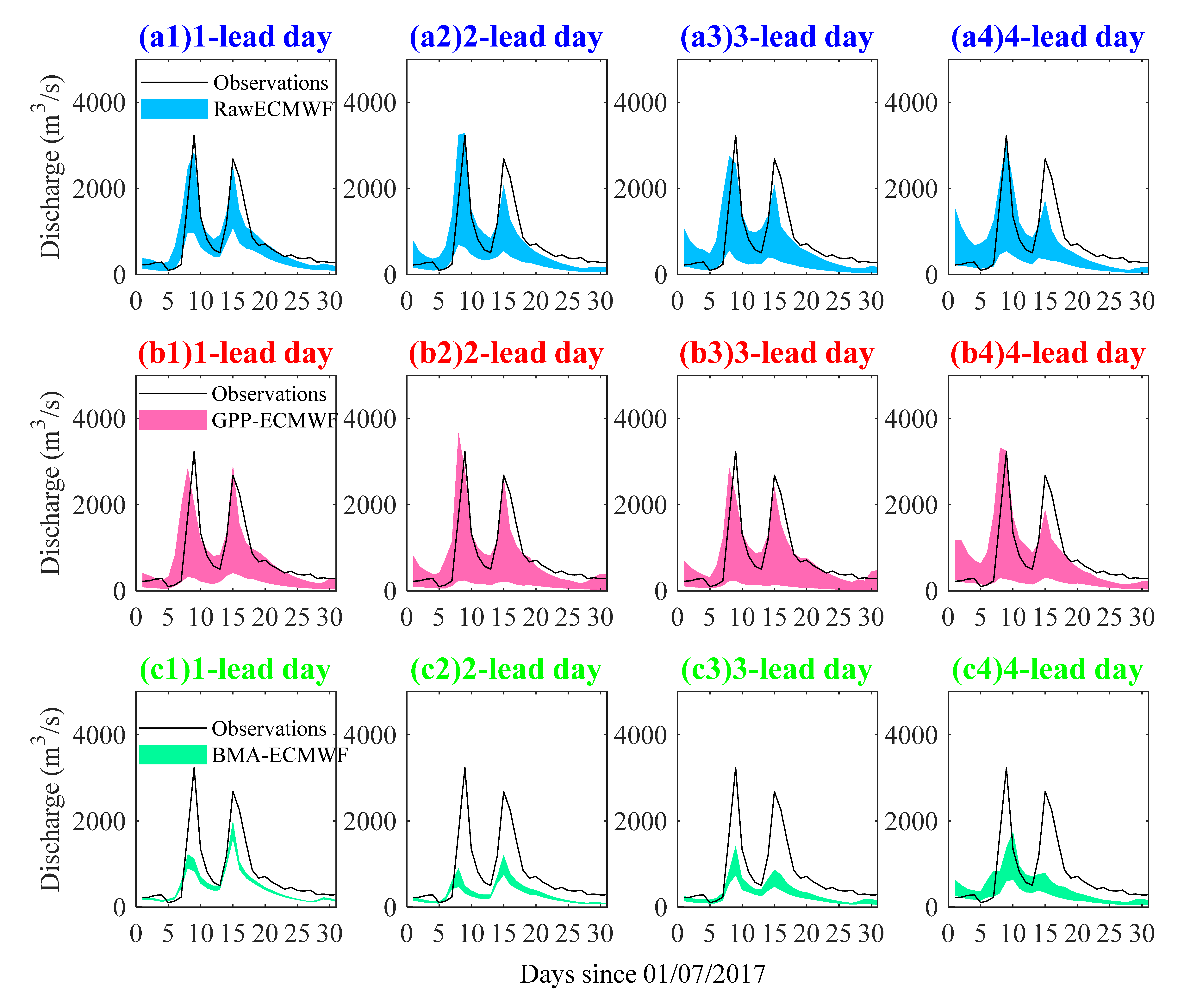
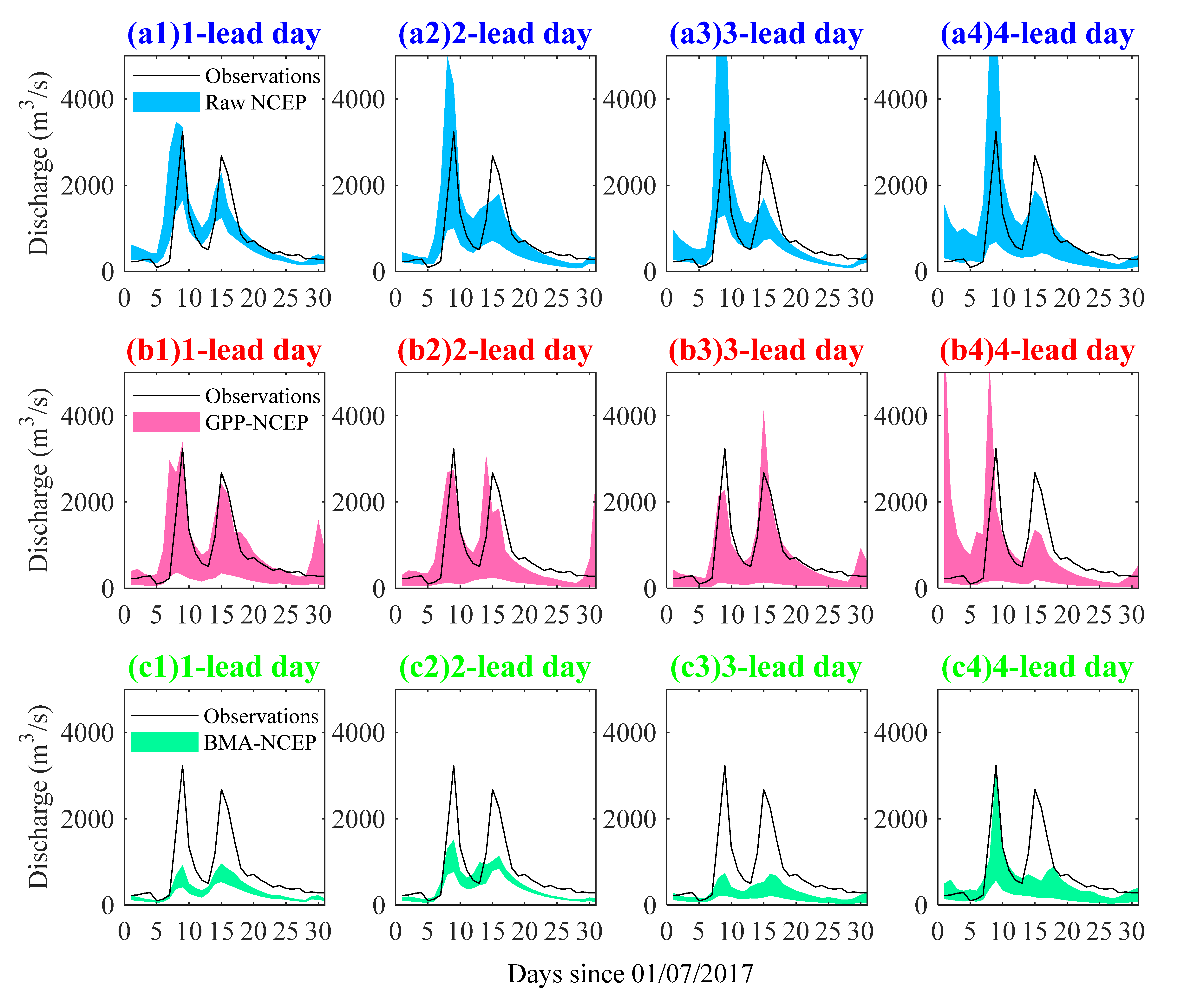
4.2. Performance of the Ensemble Streamflow Forecasts

In this section, the XAJ model was firstly calibrated to river discharge data based on meteorological observation data over the 2014–2016 period and validated over the 2017 period. Then, the ESPs were built by driving the calibrated XAJ model using raw EPFs, and postprocessed EPFs from ECMWF and NCEP, respectively.

Figure 7 presents the hydrographs of the daily simulated and observed streamflow for both calibration and validation periods; the NSE and RE are also present. It can be seen that the NSE values are both greater than 0.8 and the RE values are both below 10% for both the calibration and validation periods. In addition, the trend and magnitude of the simulated hydrograph are well-captured for both the peak and low flows. In general, the results demonstrate satisfactory performance of the XAJ model and thus can be used for streamflow forecasting.

Figure 8 presents the scatter plots of the ensemble mean forecast and observed streamflow at 1~4 lead days during the 2017 period. Figure 8a1–a12 are for ECMWF, and (Figure 8b1–b12) are for NCEP. The figure shows larger biases for forecast streamflow with the lead days increasing compared with observed streamflow. Both ECMWF and NCEP underestimate high streamflow (>2000 m³/s), which may be due to the underestimation of heavy precipitation events by EPFs (Figure 3). The use of NSE for calibrating the hydrological model could also result in underestimating peak flow events, which was theoretically demonstrated by Gupta, Kling [45]. What’s more, Tian, Booij [46] pointed out that the XAJ model was built for the regions with low surface runoff and high interflows with the concept of runoff generation on repletion of storage. While in mountainous areas, a flood could happen when the intensity of rainfall is significant without filling up the soil storage, thus leading to the underestimation of peak flow events. As for ECMWF, the performance in forecasting streamflow with low and moderate amounts (<2000 m³/s) is better than that with high amounts, with the former closer to the best-fitting line. As for NCEP, the performances are poor in forecasting streamflow with either high or low amounts, showing many data points far away from the best-fitting line. In addition, the improvements in depicting streamflow amounts are not significant for the forecasts by using the GPP method, while the performance is even worse when using the BMA method.

Table 2. CRPSS values for ensemble streamflow simulated by raw and postprocessed ECMWF and NCEP at 1~7 lead days during the 2017 period.

Lead Days	ECMWF			NCEP
	Raw	GPP	BMA	Raw	GPP	BMA
1lead day	0.62	0.59	0.29	0.49	0.54	0.28
2lead day	0.47	0.54	0.14	0.28	0.48	0.19
3lead day	0.50	0.53	0.14	0.15	0.39	0.10
4lead day	0.48	0.53	0.17	0.12	0.36	0.12
5lead day	0.47	0.50	0.17	0.17	0.38	0.15
6lead day	0.44	0.44	0.14	0.13	0.39	0.19
7lead day	0.42	0.39	0.18	0.21	0.37	0.20
Mean value	0.49	0.50	0.18	0.22	0.41	0.18

presents the CRPSS values for ensemble streamflow simulated by raw and postprocessed ECMWF and NCEP at 1~7 lead days over a 1-year period in 2017. ECMWF shows a better performance in streamflow prediction than NCEP, depicted by higher CRPSS values at all 7 lead days. According to studies of Harrigan, Prudhomme [47] and Bennett, Wang [48], the degree of ESP skill can be considered to be: very high if CRPSS is [0.75, 1]; high if CRPSS is [0.5, 0.75); moderate if CRPSS is [0.25, 0.5); low if CRPSS is (0, 0. 25); no skill if CRPSS = 0, and negative skill if CRPSS < 0. Based on that, the ESP skill of raw ECMWF is high for the first 3 lead days, and it is moderate for the latter 4 lead days. By using the GPP method, the ECMWF ESP skill is generally improved with the skill being high for 1~5 lead days. The ESP skill of raw NCEP is moderate for the first 2 lead days, and it is low for the other lead days. By using the GPP method, the NCEP ESP skill is significantly improved, with the skill being high for 1 lead day and moderate for 2~7 lead days. However, both the BMA-ECMWF and BMA-NCEP ESPs are, on average, lowly skillful for the 7 lead days. These results demonstrate the effectiveness of the GPP method in improving ESP skill, which is more significant for the NCEP with worse raw performances.

To further assess the EPF and ESP performances in extreme precipitation events, a severe flood event that occurred in July 2017 (Figure 7) was chosen. Therefore, the basin-averaged precipitation obtained from raw and postprocessed EPFs were examined against observed precipitation during the one-month period from 1 to 31 July 2017. Figure 9 presents the daily precipitation obtained from basin-averaged observations and raw forecasts at the first 4 lead days. It can be seen that observations show two peak events occurring on days 8 (86 mm) and 14 (65 mm), respectively. The peak occurrence time forecasted by raw ECMWF and NCEP both closely match the observed precipitation. Raw ECMWF forecasts lower magnitudes of precipitation relative to observations during the peak event. For the remaining days, raw ECMWF consistently forecasts higher magnitudes of precipitation. The differences between raw NCEP forecasts and observations are larger than those between raw ECMWF and observations. This is consistent with the results of Section 4.1, which reveal a better performance for ECMWF in precipitation forecasting. In addition, the forecasting uncertainty of both ECMWF and NCEP are larger for longer lead days, as indicated by the wider shade areas.

Figure 10 and Figure 11, respectively present the ensemble hydrographs simulated using raw and postprocessed ECMWF and NCEP at the first 4 lead days over the upper Qingjiang basin; the observed streamflow is also plotted. Figure 10a1–a4 show that the peak occurrence time predicted by raw ECMWF closely matches the observed streamflow. The differences in magnitude for the first peak event between predictions and observations are −11.90%, 1.74%, −14.78%, and −4.94%, at 1, 2, 3, and 4 lead days, respectively. Additionally, the differences for the second peak event are 6.57%, 22.81%, 22.31%, and 35.83%, at 1, 2, 3, and 4 lead days, respectively. The GPP-ECMWF can predict streamflow better than raw ECMWF, indicated by the reductions of both overprediction and underprediction for the two peak events at the first 3 lead days in Figure 10b1–b3. By using the GPP method, the absolute differences are lower than 13.38% and 10.54% for the first and second peak events, respectively. However, the streamflow prediction skill decreases by using the BMA method, with considerable underestimations of the two peak events demonstrated by Figure 10(c1–c4). In addition, the bias and uncertainty become larger as the number of lead days increases.

Figure 11a1–a4 show that the peak occurrence time predicted by raw NCEP closely matches the observed streamflow, just as the raw ECMWF does. As for the magnitude, the predictions at 1 lead day show 7.31% higher for the first peak event and 14.77% lower for the second peak event compared with the observations. There are considerable overestimations for the first peak event and underestimations for the second peak event at 2, 3, and 4 lead days. By using the GPP method, the NCEP forecasts at 1 and 2 lead days are improved in terms of representing the hydrograph. The absolute differences are lower than 13.41% and 14.89% for the first and second peak events, respectively. By using the BMA method, the magnitude of predicted streamflow is much smaller than observations. Similarly, the performance of the NCEP forecasts decreases as lead days increase. These results of Figure 10 and Figure 11 demonstrate that the ECMWF performs better than NCEP in flood prediction; the GPP method performs better than the BMA method in improving the prediction skill. The skillful forecast lead time can be 3 days/2 days for GPP-ECMWF/GPP-NCEP flood predictions, with differences in magnitude of less than 15%. It is shorter than the 5 lead days of NCEP for flood season streamflow predictions pointed out by Zhang, Chen [25]. This is due to difficulties in estimating precipitation in the mountain river basin in our evaluation.

5. Conclusions

This study evaluated the performances of EPF and ESP for raw and postprocessed ensemble precipitation obtained from ECMWF and NCEP over a mountain river basin. The GPP and BMA methods were used to postprocess EPFs and the XAJ model was used in building ESPs. Both the deterministic and probabilistic metrics, MAE and CRPSS, were chosen to evaluate the forecasting performances. The following conclusions can be drawn:

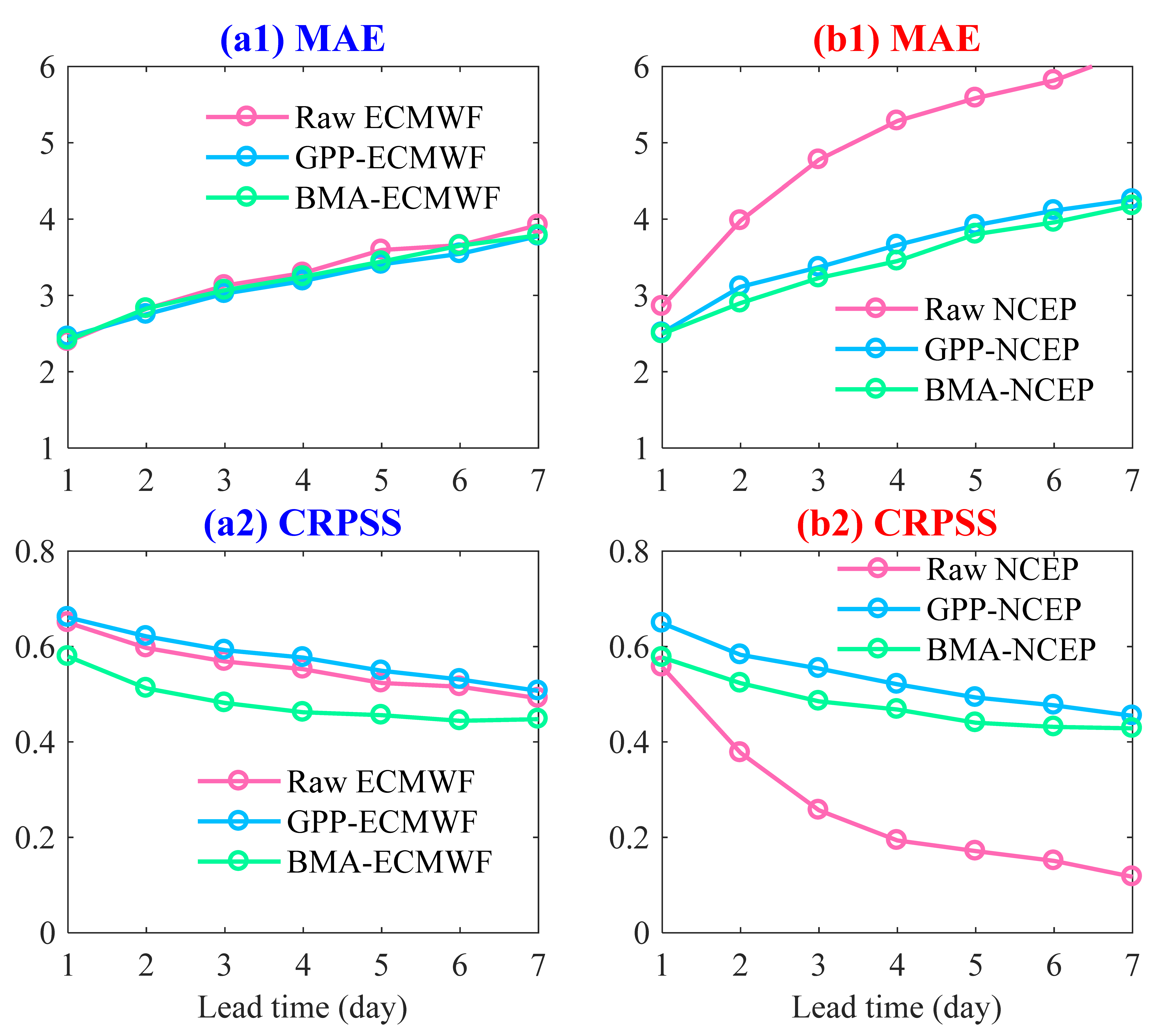
• Raw ECMWF shows a better performance in EPF than raw NCEP in terms of lower MAE and higher CRPSS at all 7 lead days. Raw ECMWF also shows a better performance in ESP with high skill for 1~3 lead days, and both magnitudes and peak occurrence time of peak events were captured better.
• The GPP method performs better than BMA in improving both EPF and ESP performances, and the improvements are more significant for the NCEP with worse raw performances.
• Both ECMWF and NCEP have good potential for both EPF and ESP. By using the GPP method, MAE values are lower than 4.2 and CRPSS values are higher than 0.43 for both ECMWF and NCEP EPFs at all 7 lead days. The GPP-ECMWF ESP is highly skillful for 1~5 lead days and the GPP-NCEP ESP is, on average, moderately skillful for 1~7 lead days. In addition, the skillful forecast lead time can be 3 days/2 days for GPP-ECMWF/GPP-NCEP flood predications, with absolute differences in magnitude of less than 15% for peak events.

Overall, this study revealed the potential of ECMWF and NCEP in medium-term precipitation and streamflow forecasting over a mountain river basin and showed the effectiveness of the GPP method in improving forecast skill. There are still some limitations. Previous studies [28,39] showed that the ensemble of multiple EPFs based on combination methods exhibited better forecast skill than the single EPF. Therefore, further work is needed to investigate the forecast skill of the ensemble of multiple EPFs. In addition, only one hydrological model was adopted for streamflow forecasting, even though hydrological prediction accuracy is influenced by different hydrological models [25,28]. This lack of consideration is because the purpose of this study is mainly to investigate the ESP performances related to different precipitation inputs and postprocessing methods. The uncertainty in streamflow prediction related to hydrological models will be investigated in our future study.

References

1. Roulin, E. Skill and Relative Economic Value of Medium-Range Hydrological Ensemble Predictions. Hydrol. Earth Syst. Sci. 2007, 11, 725–737. [Google Scholar] [CrossRef] [Green Version]
2. Shukla, S.; Voisin, N.; Lettenmaier, D.P. Value of Medium Range Weather Forecasts in the Improvement of Seasonal Hydrologic Prediction Skill. Hydrol. Earth Syst. Sci. 2012, 16, 2825–2838. [Google Scholar] [CrossRef] [Green Version]
3. Xu, Y.-P.; Tung, Y.-K. Decision-Making In Water Management Under Uncertainty. Water Resour. Manag. 2008, 22, 535–550. [Google Scholar] [CrossRef]
4. Alfieri, L.; Pappenberger, F.; Wetterhall, F.; Haiden, T.; Richardson, D.; Salamon, P. Evaluation of Ensemble Streamflow Predictions in Europe. J. Hydrol. 2014, 517, 913–922. [Google Scholar] [CrossRef] [Green Version]
5. Tao, Y.; Duan, Q.; Ye, A.; Gong, W.; Di, Z.; Xiao, M.; Hsu, K. An Evaluation Of Post-Processed TIGGE Multimodel Ensemble Precipitation Forecast in the Huai River Basin. J. Hydrol. 2014, 519, 2890–2905. [Google Scholar] [CrossRef] [Green Version]
6. Swinbank, R.; Kyouda, M.; Buchanan, P.; Froude, L.; Hamill, T.M.; Hewson, T.D.; Keller, J.H.; Matsueda, M.; Methven, J.; Yamaguchi, M.; et al. The TIGGE Project and Its Achievements. Bull. Am. Meteorol. Soc. 2016, 97, 49–67. [Google Scholar] [CrossRef]
7. Weidle, F.; Wang, Y.; Smet, G. On the Impact of the Choice of Global Ensemble in Forcing a Regional Ensemble System. Weather. Forecast. 2016, 31, 515–530. [Google Scholar] [CrossRef]
8. Titley, H.A.; Bowyer, R.L.; Cloke, H.L. A Global Evaluation Of Multi-Model Ensemble Tropical Cyclone Track Probability Forecasts. Q. J. R. Meteorol. Soc. 2020, 146, 531–545. [Google Scholar] [CrossRef]
9. Qu, B.; Zhang, X.; Pappenberger, F.; Zhang, T.; Fang, Y. Multi-Model Grand Ensemble Hydrologic Forecasting in the Fu River Basin Using Bayesian Model Averaging. Water 2017, 9, 74. [Google Scholar] [CrossRef]
10. Cloke, H.L.; Pappenberger, F. Ensemble Flood Forecasting: A Review. J. Hydrol. 2009, 375, 613–626. [Google Scholar] [CrossRef]
11. He, Y.; Wetterhall, F.; Cloke, H.L.; Pappenberger, F.; Wilson, M.; Freer, J.; McGregor, G. Tracking the Uncertainty in Flood Alerts Driven by Grand Ensemble Weather Predictions. Meteorol. Appl. A J. Forecast. Pract. Appl. Train. Tech. Model. 2009, 16, 91–101. [Google Scholar] [CrossRef] [Green Version]
12. Bertotti, L.; Bidlot, J.R.; Buizza, R.; Cavaleri, L.; Janousek, M. Deterministic and Ensemble-Based Prediction of Adriatic Sea Sirocco Storms Leading to ‘Acqua Alta’in Venice. Q. J. R. Meteorol. Soc. 2011, 137, 1446–1466. [Google Scholar] [CrossRef]
13. Hagedorn, R.; Hamill, T.M.; Whitaker, J.S. Probabilistic Forecast Calibration Using ECMWF and GFS Ensemble Reforecasts. Part I: Two-Meter Temperatures. Mon. Weather. Rev. 2008, 136, 2608–2619. [Google Scholar] [CrossRef]
14. Scheuerer, M.; Hamill, T.M. Statistical Postprocessing of Ensemble Precipitation Forecasts by Fitting Censored, Shifted Gamma Distributions. Mon. Weather. Rev. 2015, 143, 4578–4596. [Google Scholar] [CrossRef]
15. Vetter, T.; Reinhardt, J.; Flörke, M.; Van Griensven, A.; Hattermann, F.; Huang, S.; Koch, H.; Pechlivanidis, I.G.; Plötner, S.; Seidou, O.; et al. Evaluation of Sources of Uncertainty in Projected Hydrological Changes Under Climate Change in 12 Large-Scale River Basins. Clim. Chang. 2017, 141, 419–433. [Google Scholar] [CrossRef]
16. Wilks, D.S. Comparison of Ensemble-MOS Methods in the Lorenz’96 Aetting. Meteorol. Appl. 2006, 13, 243–256. [Google Scholar] [CrossRef]
17. Raftery, A.E.; Gneiting, T.; Balabdaoui, F.; Polakowski, M. Using Bayesian Model Averaging to Calibrate Forecast Ensembles. Mon. Weather. Rev. 2005, 133, 1155–1174. [Google Scholar] [CrossRef] [Green Version]
18. Roulin, E.; Vannitsem, S. Postprocessing of Ensemble Precipitation Predictions with Extended Logistic Regression Based on Hindcasts. Mon. Weather. Rev. 2012, 140, 874–888. [Google Scholar] [CrossRef]
19. Chen, J.; Brissette, F.P.; Li, Z. Postprocessing of Ensemble Weather Forecasts Using a Stochastic Weather Generator. Mon. Weather. Rev. 2014, 142, 1106–1124. [Google Scholar] [CrossRef]
20. Grönquist, P.; Yao, C.; Ben-Nun, T.; Dryden, N.; Dueben, P.; Li, S.; Hoefler, T. Deep Learning For Post-Processing Ensemble Weather Forecasts. Philos. Trans. R. Soc. A 2021, 379, 20200092. [Google Scholar] [CrossRef]
21. Zhao, P.; Wang, Q.J.; Wu, W.; Yang, Q. Extending a Joint Probability Modelling Approach for Post-Processing Ensemble Precipitation Forecasts from Numerical Weather Prediction Models. J. Hydrol. 2022, 605, 127285. [Google Scholar] [CrossRef]
22. Boucher, M.A.; Perreault, L.; Anctil, F.; Favre, A.C. Exploratory Analysis of Statistical Post-Processing Methods for Hydrological Ensemble Forecasts. Hydrol. Processes 2015, 29, 1141–1155. [Google Scholar] [CrossRef]
23. Schmeits, M.J.; Kok, K.J. A Comparison Between Raw Ensemble Output, (Modified) Bayesian Model Averaging, and Extended Logistic Regression Using ECMWF Ensemble Precipitation Reforecasts. Mon. Weather. Rev. 2020, 138, 4199–4211. [Google Scholar] [CrossRef]
24. Li, Y.; Jiang, Y.; Lei, X.; Tian, F.; Duan, H.; Lu, H. Comparison of Precipitation And Streamflow Correcting For Ensemble Streamflow Forecasts. Water 2018, 10, 177. [Google Scholar] [CrossRef] [Green Version]
25. Zhang, J.; Chen, J.; Li, X.; Chen, H.; Xie, P.; Li, W. Combining Postprocessed Ensemble Weather Forecasts And Multiple Hydrological Models For Ensemble Streamflow Predictions. J. Hydrol. Eng. 2020, 25, 04019060. [Google Scholar] [CrossRef]
26. Su, X.; Yuan, H.; Zhu, Y.; Luo, Y.; Wang, Y. Evaluation of TIGGE Ensemble Predictions of Northern Hemisphere Summer Precipitation During 2008–2012. J. Geophys. Res. Atmos. 2014, 119, 7292–7310. [Google Scholar] [CrossRef]
27. Qi, H.; Zhi, X.; Peng, T.; Bai, Y.; Lin, C. Comparative Study on Probabilistic Forecasts of Heavy Rainfall in Mountainous Areas of the Wujiang River Basin in China Based On TIGGE Data. Atmosphere 2019, 10, 608. [Google Scholar] [CrossRef] [Green Version]
28. Shu, Z.; Zhang, J.; Jin, J.; Wang, L.; Wang, G.; Wang, J.; Sun, Z.; Liu, J.; Liu, Y.; He, H.; et al. Evaluation and Application of Quantitative Precipitation Forecast Products for Mainland China Based on TIGGE Multimodel Data. J. Hydrometeorol. 2021, 22, 1199–1219. [Google Scholar] [CrossRef]
29. Liu, X.; Zhang, L.; She, D.; Chen, J.; Xia, J.; Chen, X.; Zhao, T. Postprocessing of Hydrometeorological Ensemble Forecasts Based On Multisource Precipitation In Ganjiang River Basin, China. J. Hydrol. 2022, 605, 127323. [Google Scholar] [CrossRef]
30. Liu, L.; Gao, C.; Zhu, Q.; Xu, Y.P. Evaluation of TIGGE Daily Accumulated Precipitation Forecasts Over the Qu River Basin, China. J. Meteorol. Res. 2019, 33, 747–764. [Google Scholar] [CrossRef]
31. Peng, T.; Qi, H.; Wang, J. Case Study on Extreme Flood Forecasting Based on Ensemble Precipitation Forecast in Qingjiang Basin of the Yangtze River. J. Coast. Res. 2020, 104, 178–187. [Google Scholar] [CrossRef]
32. Li, X.Q.; Chen, J.; Xu, C.Y.; Li, L.; Chen, H. Performance of post-processed methods in hydrological predictions evaluated by deterministic and probabilistic criteria. Water Resour. Manag. 2019, 33, 3289–3302. [Google Scholar] [CrossRef]
33. Sloughter, J.M.L.; Raftery, A.E.; Gneiting, T.; Fraley, C. Probabilistic Quantitative Precipitation Forecasting Using Bayesian Model Averaging. Mon. Weather. Rev. 2007, 135, 3209–3220. [Google Scholar] [CrossRef]
34. Ren-Jun, Z. The Xinanjiang model applied in China. J. Hydrol. 1992, 135, 371–381. [Google Scholar] [CrossRef]
35. Xiang, Y.; Chen, J.; Li, L.; Peng, T.; Yin, Z. Evaluation of Eight Global Precipitation Datasets in Hydrological Modeling. Remote Sens. 2021, 13, 2831. [Google Scholar] [CrossRef]
36. Duan, Q.Y.; Gupta, V.K.; Sorooshian, S. Shuffled Complex Evolution Approach for Effective and Efficient Global Minimization. J. Optim. Theory Appl. 1993, 76, 501–521. [Google Scholar] [CrossRef]
37. Nash, J.E.; Sutcliffe, J.V. River Flow Forecasting Through Conceptual Models Part I—A Discussion of Principles. J. Hydrol. 1970, 10, 282–290. [Google Scholar] [CrossRef]
38. Brown, J.D.; Demargne, J.; Seo, D.J.; Liu, Y. The Ensemble Verification System (EVS): A Software Tool For Verifying Ensemble Forecasts of Hydrometeorological and Hydrologic Variables at Discrete Locations. Environ. Model. Softw. 2010, 25, 854–872. [Google Scholar] [CrossRef]
39. Ma, F.; Ye, A.; Deng, X.; Zhou, Z.; Liu, X.; Duan, Q.; Xu, J.; Miao, C.; Di, Z.; Gong, W. Evaluating the Skill of NMME Seasonal Precipitation Ensemble Predictions for 17 Hydroclimatic Regions in Continental China. Int. J. Climatol. 2016, 36, 132–144. [Google Scholar] [CrossRef]
40. Swets, J.A. The Relative Operating Characteristic in Psychology: A Technique for Isolating Effects of Response Bias Finds Wide Use in the Study of Perception and Cognition. Science 1973, 182, 990–1000. [Google Scholar] [CrossRef]
41. Mason, S.J.; Graham, N.E. Conditional Probabilities, Relative Operating Characteristics, and Relative Operating Levels. Weather. Forecast. 1999, 14, 713–725. [Google Scholar] [CrossRef]
42. Liu, C.; Sun, J.; Yang, X.; Jin, S.; Fu, S. Evaluation of ECMWF Precipitation Predictions in China during 2015–18. Weather. Forecast. 2021, 36, 1043–1060. [Google Scholar] [CrossRef]
43. Huang, L.; Luo, Y. Evaluation of Quantitative Precipitation Forecasts By TIGGE Ensembles for South China During The Presummer Rainy Season. J. Geophys. Res. Atmos. 2017, 122, 8494–8516. [Google Scholar] [CrossRef]
44. Jha, S.K.; Shrestha, D.L.; Stadnyk, T.A.; Coulibaly, P. Evaluation of Ensemble Precipitation Forecasts Generated Through Post-Processing in a Canadian Catchment. Hydrol. Earth Syst. Sci. 2018, 22, 1957–1969. [Google Scholar] [CrossRef] [Green Version]
45. Gupta, H.V.; Kling, H.; Yilmaz, K.K.; Martinez, G.F. Decomposition of the Mean Squared Error and NSE Performance Criteria: Implications for Improving Hydrological Modelling. J. Hydrol. 2009, 377, 80–91. [Google Scholar] [CrossRef] [Green Version]
46. Tian, Y.; Booij, M.J.; Xu, Y.P. Uncertainty in High and Low Flows Due to Model Structure and Parameter Errors. Stoch. Environ. Res. Risk Assess. 2014, 28, 319–332. [Google Scholar] [CrossRef]
47. Harrigan, S.; Prudhomme, C.; Parry, S.; Smith, K.; Tanguy, M. Benchmarking Ensemble Streamflow Prediction Skill in the UK. Hydrol. Earth Syst. Sci. 2018, 22, 2023–2039. [Google Scholar] [CrossRef] [Green Version]
48. Bennett, J.C.; Wang, Q.J.; Robertson, D.E.; Schepen, A.; Li, M.; Michael, K. Assessment of an Ensemble Seasonal Streamflow Forecasting System for Australia. Hydrol. Earth Syst. Sci. 2017, 21, 6007–6030. [Google Scholar] [CrossRef] [Green Version]
Figure 1. The study area.
Water 14 02432 g001
Figure 2. Flowchart of the XAJ model.
Water 14 02432 g002
Figure 3. Comparison of daily observed precipitation and raw EPFs from ECMWF (a1,a2) and NCEP (b1,b2) at 1 lead day during 2017. (a1,b1) are the time series of forecast and observed precipitation; (a2,b2) are the scatter plots of ensemble mean forecast and observed precipitation.
Water 14 02432 g003
Figure 4. Line chart of evaluation indexes for ensemble precipitation forecasts by raw and postprocessed ECMWF (a1,a2) and NCEP (b1,b2).
Water 14 02432 g004
Figure 5. Monthly variation of evaluation indexes for ensemble precipitation forecasts by raw and postprocessed ECMWF (a1,a2) and NCEP (b1,b2).
Water 14 02432 g005
Figure 6. Relative operating characteristic (ROC) curve at 1, 3, 5, and 7lead days for ECMWF (solid line) and NCEP (dash line) for events of precipitation greater than 50 mm (the FPR is the hit rate of no-event “0”, and the TPR is the hit rate of event “1”). In the calculation of ROC, the daily data of 2017 were used.
Water 14 02432 g006
Figure 7. Hydrographs simulated by XAJ model in calibration and validation periods, compared with daily observations.
Water 14 02432 g007
Figure 8. Scatter plots of ensemble mean forecast and observed streamflow during the 2017 period. (a1a12) represent ECMWF and (b1b12) represent NCEP. Columns 1–4 represent 1, 2, 3, and 4 lead days, respectively.
Water 14 02432 g008
Figure 9. Comparison of time series of precipitation obtained from basin-averaged raw ECMWF (blue color) and NCEP (pink color) at 1, 2, 3, and 4 lead days, with observed precipitation. The shaded area represents the 5th–95th percentile values obtained from 1000 postprocessed ensembles.
Water 14 02432 g009
Figure 10. Hydrographs of ensemble streamflow simulated by XAJ model using raw and postprocessed EPFs from ECMWF as inputs at 1, 2, 3, and 4 lead days, compared with observed streamflow. The shaded area represents the 5th–95th percentile values driving by 1000 postprocessed ensembles.
Water 14 02432 g010
Figure 11. Hydrographs of ensemble streamflow simulated by XAJ model using raw and postprocessed EPFs from NCEP as inputs at 1, 2, 3, and 4 lead days, compared with observed streamflow. The shaded area represents the 5th–95th percentile values driving by 1000 postprocessed ensembles.
Water 14 02432 g011