
Effects of the Digital Elevation Model and Hydrological Processing Algorithms on the Geomorphological Parameterization


 ,
,  , ,
, ,  ,
,  and
and 
Abstract
1. Introduction
2. Methodology
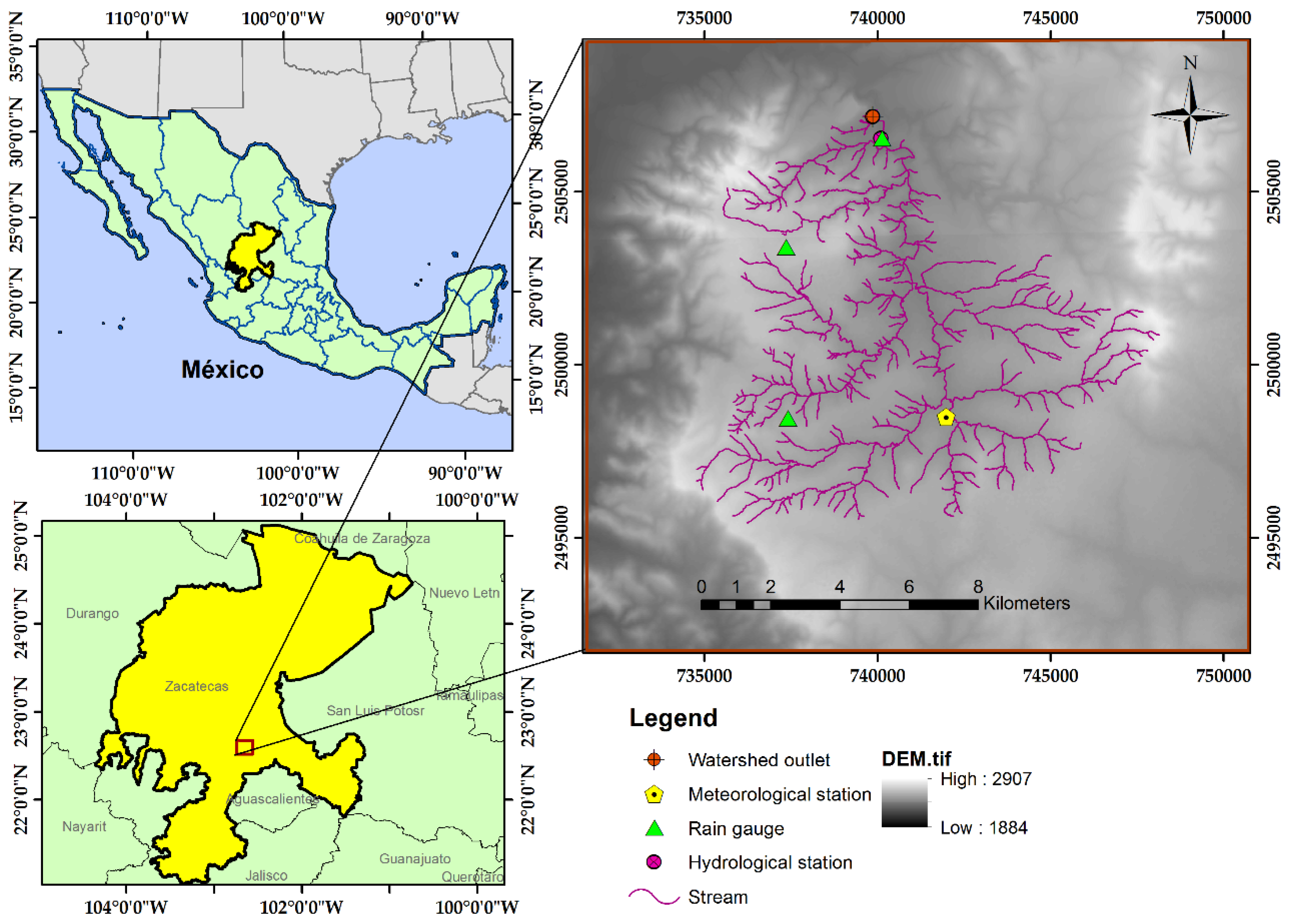
2.1. Study Site
2.2. Data Set Used
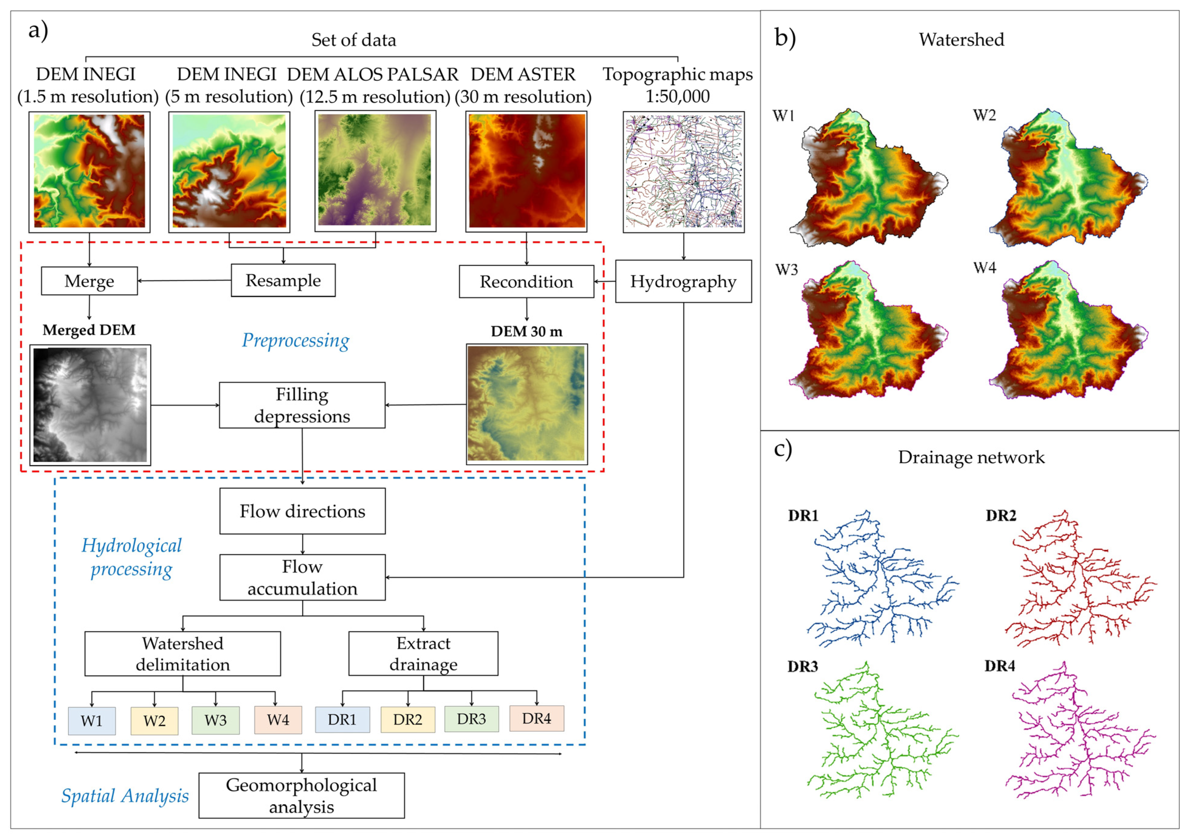
2.3. Geomorphological Parameterization
2.3.1. Preprocessing
Filling Depressions
2.3.2. Hydrological Processing
Flow Directions
Flow Accumulation
Determination of Drainage Network and Watershed Delimitation
Geomorphological Parameters Quantification
3. Results and Discussions
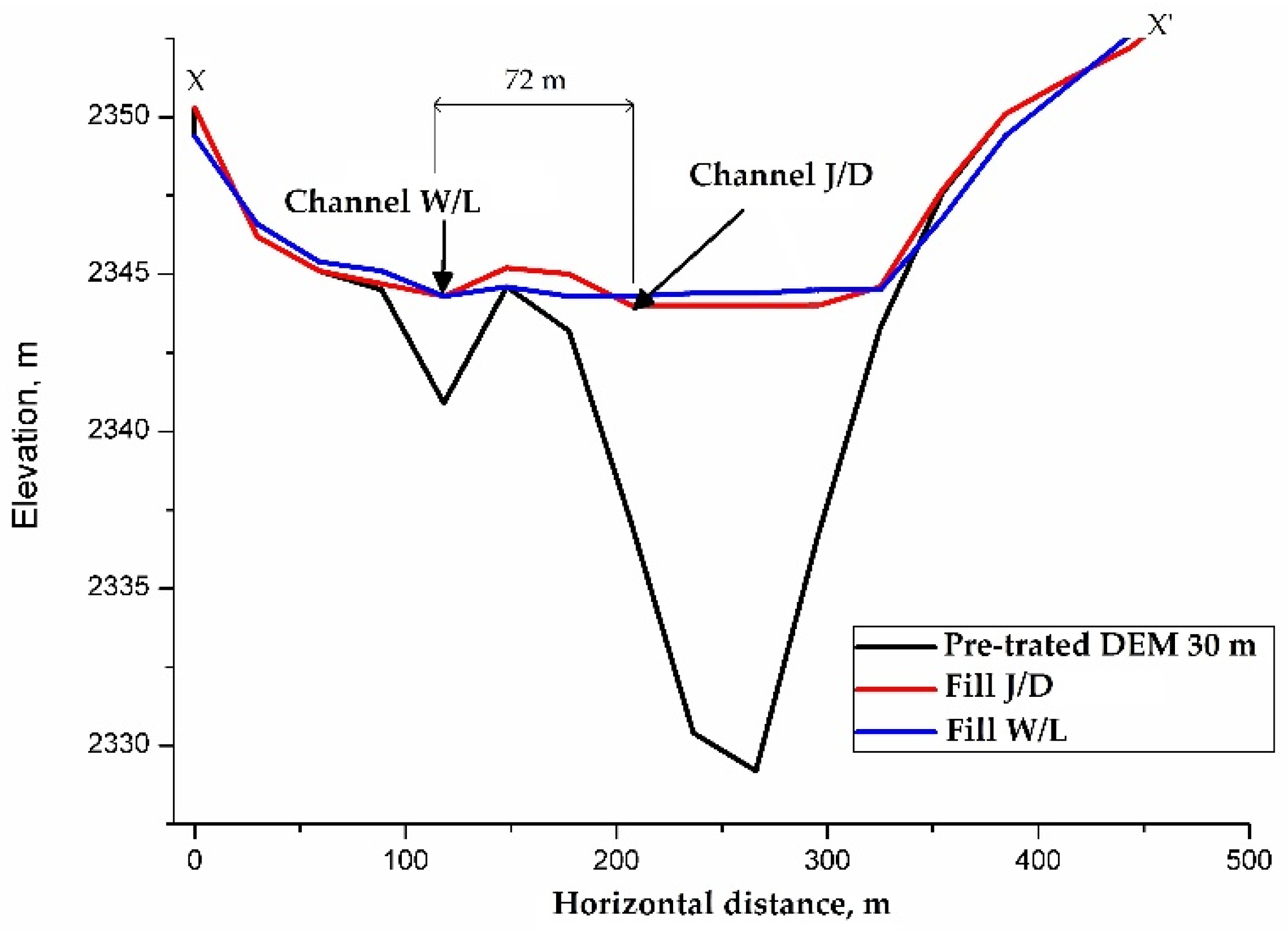
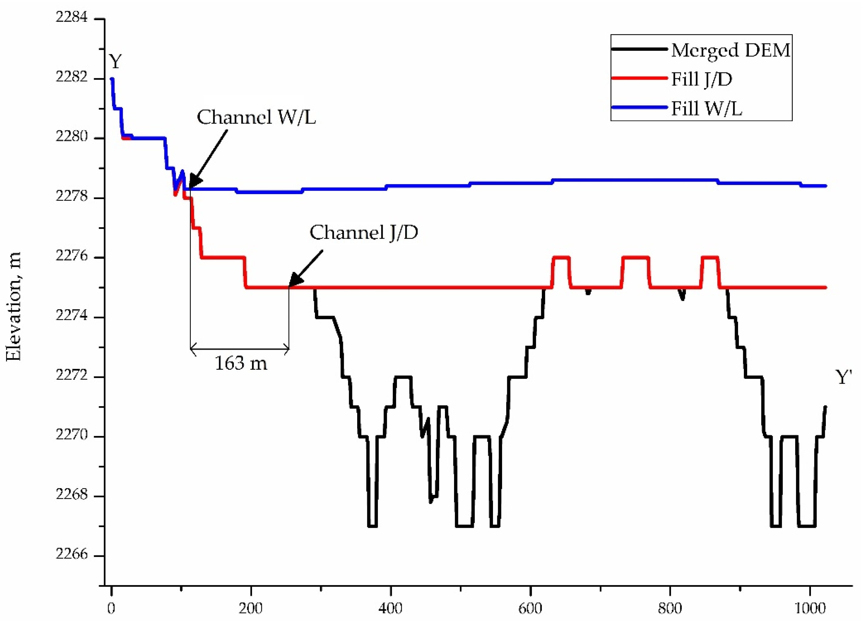
3.1. Comparative of Fill DEMs
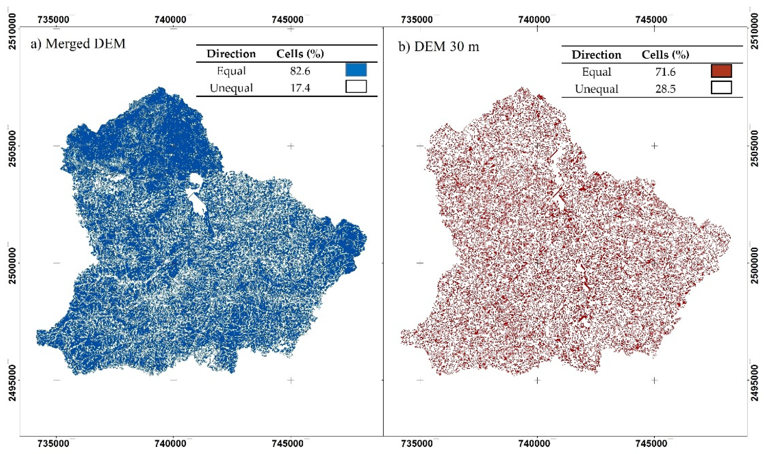
3.2. DEM Comparison Flow Direction
3.3. Geomorphometric Parameterization
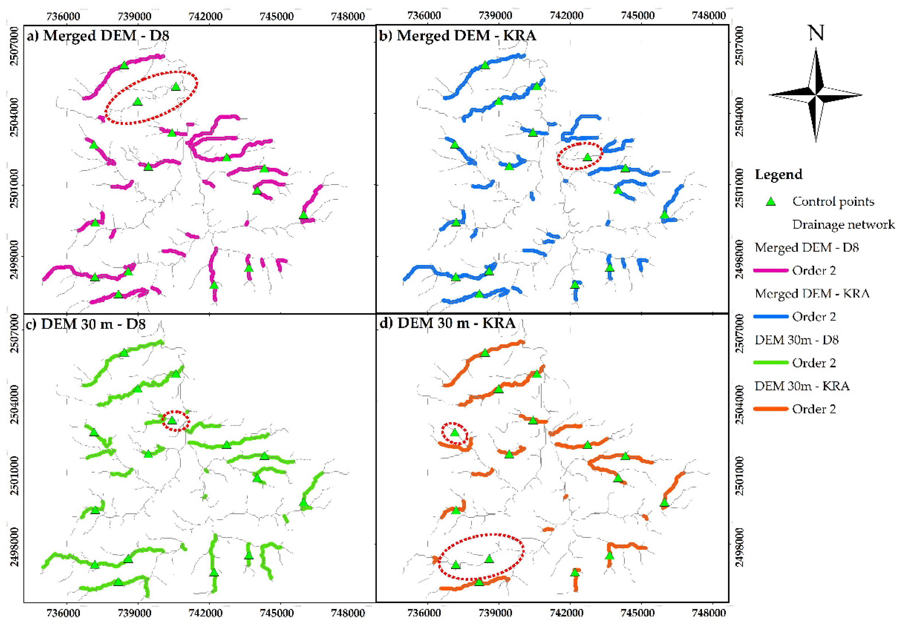
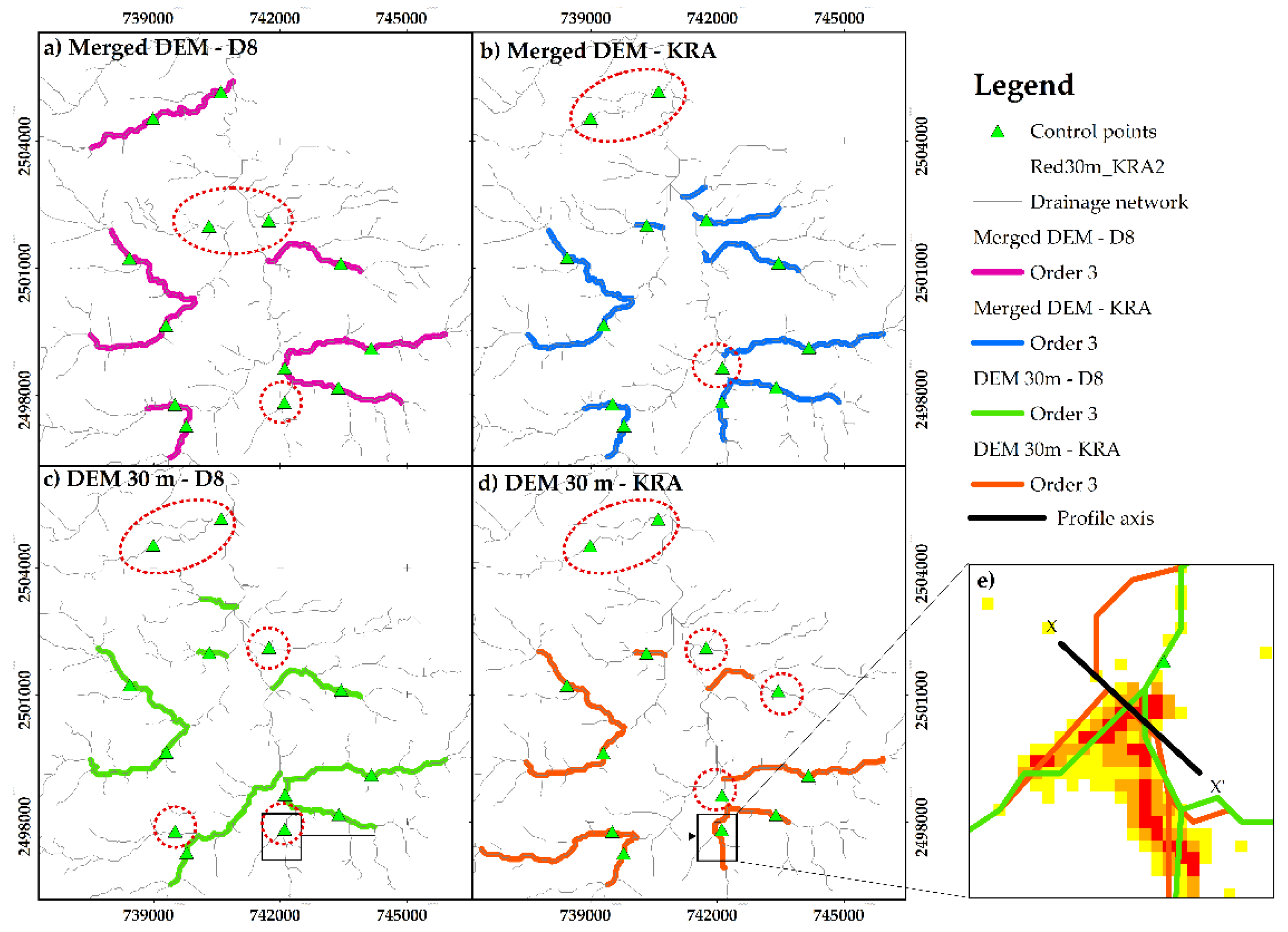
3.4. Drainage Networks Analysis
4. Conclusions
Author Contributions
Funding
Institutional Review Board Statement
Informed Consent Statement
Data Availability Statement
Acknowledgments
Conflicts of Interest
References
- Altaf, F.; Meraj, G.; Romshoo, S.A. Morphometric Analysis to Infer Hydrological Behaviour of Lidder Watershed, Western Himalaya, India. Geogr. J. 2013, 2013, 1–14. [Google Scholar] [CrossRef]
- Beven, K. Searching for the Holy Grail of Scientific Hydrology: Qt= H(SR)A as closure. Hydrol. Earth Syst. Sci. 2006, 3, 769–792. [Google Scholar] [CrossRef]
- Krishnamurthy, J.; Srinivas, G.; Jayaraman, V.; Chandrasekhar, M.G. Influence of Rock Types and Structures in Development of Drainage Network in Typical Hardrock Terrain. Int. J. Appl. Earth Obs. Geoinf. 1996, 3/4, 252–259. [Google Scholar]
- Pareta, K.; Pareta, U. Quantitative morphometric analysis of a watershed of Yamuna basin, India using ASTER (DEM) data and GIS. Int. J. Geomat. Geosci. 2011, 2, 248. [Google Scholar]
- Costabile, P.; Costanzo, C.; Ferraro, D.; Macchione, F.; Petaccia, G. Performances of the New HEC-RAS Version 5 for 2-D Hydrodynamic-Based Rainfall-Runoff Simulations at Basin Scale: Comparison with a State-of-the Art Model. Water 2020, 12, 2326. [Google Scholar] [CrossRef]
- Engelhardt, B.M.; Weisberg, P.J.; Chambers, J.C.; Huston, M. Influences of watershed geomorphology on extent and composition of riparian vegetation. J. Veg. Sci. 2012, 23, 127–139. [Google Scholar] [CrossRef]
- García, A.; Acosta, J.; Chávez, E.; Yuli Posadas, R.; Bulege, W. Use of Hydrogeomorphic Indexes in SAGA-GIS for the Characterization of Flooded Areas in Madre de Dios, Peru. Int. J. Appl. Eng. Res. 2017, 12, 9078–9086. [Google Scholar]
- Pilesjö, P.; Hasan, A. A Triangular Form-based Multiple Flow Algorithm to Estimate Overland Flow Distribution and Accumulation on a Digital Elevation Model. Trans. GIS 2014, 18, 108–124. [Google Scholar] [CrossRef]
- Tesfa, T.K.; Tarboton, D.G.; Watson, D.W.; Schreuders, K.A.T.; Baker, M.E.; Wallace, R.M. Extraction of hydrological proximity measures from DEMs using parallel processing. Environ. Model. Softw. 2011, 26, 1696–1709. [Google Scholar] [CrossRef]
- Diakakis, M. A method for flood hazard mapping based on basin morphometry: Application in two catchments in Greece. Nat. Hazards 2010, 56, 803–814. [Google Scholar] [CrossRef]
- Huang, P.-C.; Lee, K.T. Influence of topographic features and stream network structure on the spatial distribution of hydrological response. J. Hydrol. 2021, 603, 126856. [Google Scholar] [CrossRef]
- Costabile, P.; Costanzo, C.; De Bartolo, S.; Gangi, F.; Macchione, F.; Tomasicchio, G. Hydraulic Characterization of River Networks Based on Flow Patterns Simulated by 2-D Shallow Water Modeling: Scaling Properties, Multifractal Interpretation, and Perspectives for Channel Heads Detection. Water Resour. Res. 2019, 55, 7717–7752. [Google Scholar] [CrossRef]
- López-Vicente, M.; Navas, A. Routing runoff and soil particles in a distributed model with GIS: Implications for soil protection in mountain agricultural landscapes. Land Degrad. Dev. 2010, 21, 100–109. [Google Scholar] [CrossRef]
- Vozinaki, A.-E.K.; Morianou, G.G.; Alexakis, D.D.; Tsanis, I.K. Comparing 1D and combined 1D/2D hydraulic simulations using high-resolution topographic data: A case study of the Koiliaris basin, Greece. Hydrol. Sci. J. 2016, 62, 642–656. [Google Scholar] [CrossRef]
- Pardo-Igúzquiza, E.; Dowd, P.A. The mapping of closed depressions and its contribution to the geodiversity inventory. Int. J. Geoheritage Parks 2021, 9, 480–495. [Google Scholar] [CrossRef]
- Patel, D.P.; Gajjar, C.A.; Srivastava, P.K. Prioritization of Malesari mini-watersheds through morphometric analysis: A remote sensing and GIS perspective. Environ. Earth Sci. 2012, 69, 2643–2656. [Google Scholar] [CrossRef]
- Chen, H.; Liang, Q.; Liu, Y.; Xie, S. Hydraulic correction method (HCM) to enhance the efficiency of SRTM DEM in flood modeling. J. Hydrol. 2018, 559, 56–70. [Google Scholar] [CrossRef]
- Prieto, A.; Pinedo, A.; Vázquez, Q.; Valles, A.; Rascón, R.; Martinez, S.; Villarreal, G. A Multivariate Geomorphometric Approach to Prioritize Erosion-Prone Watersheds. Sustainability 2019, 11, 5140. [Google Scholar] [CrossRef]
- Brunda, G.S.; Nyamathi, S.J. Derivation and Analysis of Dimensionless Hydrograph and S Curve for Cumulative Watershed Area. Aquat. Procedia 2015, 4, 964–971. [Google Scholar] [CrossRef]
- Burke, L.; Sugg, Z. Hydrologic Modeling of Watersheds Discharging Adjacent to the Mesoamerican Reef; World Resources Institute: Washington, DC, USA, 2006; p. 36. [Google Scholar]
- Chang, C.-H.; Lee, K.T. Analysis of geomorphologic and hydrological characteristics in watershed saturated areas using topographic-index threshold and geomorphology-based runoff model. Hydrol. Processes 2008, 22, 802–812. [Google Scholar] [CrossRef]
- Goñi, M.; López, J.J.; Gimena, F.N. Geomorphological instantaneous unit hydrograph model with distributed rainfall. Catena 2019, 172, 40–53. [Google Scholar] [CrossRef]
- Ji, P.; Yuan, X.; Liang, X.-Z. Do Lateral Flows Matter for the Hyperresolution Land Surface Modeling? J. Geophys.Res. Atmos. 2017, 122, 12077–12092. [Google Scholar] [CrossRef]
- O’Callaghan, J.F.; Mark, D.M.J.C. The extraction of drainage networks from digital elevation data. Comput. Vis.Graph. Image Processing 1984, 28, 323–344. [Google Scholar] [CrossRef]
- Orlandini, S.; Moretti, G. Determination of surface flow paths from gridded elevation data. Water Resour. Res. 2009, 45, 1–14. [Google Scholar] [CrossRef]
- Orlandini, S.; Moretti, G.; Franchini, M.; Aldighieri, B.; Testa, B. Path-based methods for the determination of nondispersive drainage directions in grid-based digital elevation models. Water Resour. Res. 2003, 39, 1–8. [Google Scholar] [CrossRef]
- Orlandini, S.; Moretti, G.; Gavioli, A. Analytical basis for determining slope lines in grid digital elevation models. Water Resour. Res. 2014, 50, 526–539. [Google Scholar] [CrossRef]
- Sabzevari, T.; Noroozpour, S. Effects of hillslope geometry on surface and subsurface flows. Hydrogeol. J. 2014, 22, 1593–1604. [Google Scholar] [CrossRef]
- Sabzevari, T.; Saghafian, B.; Talebi, A.; Ardakanian, R. Time of concentration of surface flow in complex hillslopes. J. Hydrol. Hydromech. 2013, 61, 269–277. [Google Scholar] [CrossRef][Green Version]
- Sadeghi, S.H.; Moradi Dashtpagerdi, M.; Moradi Rekabdarkoolai, H.; Schoorl, J.M. Sensitivity analysis of relationships between hydrograph components and landscapes metrics extracted from digital elevation models with different spatial resolutions. Ecol. Indic. 2021, 121, 107025. [Google Scholar] [CrossRef]
- Tarboton, D.G. A new method for the determination of flow directions and upslope areas in grid digital elevation models. Water Resour. Res. 1997, 33, 309–319. [Google Scholar] [CrossRef]
- Tarboton, D.G.; Bras, R.L. Rodriguez-Iturbe, On the extraction of channel networks from digital elevation data. Hydrol. Processes 1991, 5, 81–100. [Google Scholar] [CrossRef]
- Zhu, Q.; Abdelkareem, M. Mapping Groundwater Potential Zones Using a Knowledge-Driven Approach and GIS Analysis. Water 2021, 13, 579. [Google Scholar] [CrossRef]
- López-Vicente, M.; García-Ruiz, R.; Guzmán, G.; Vicente-Vicente, J.L.; Van Wesemael, B.; Gómez, J.A. Temporal stability and patterns of runoff and runon with different cover crops in an olive orchard (SW Andalusia, Spain). Catena 2016, 147, 125–137. [Google Scholar] [CrossRef]
- López-Vicente, M.; Pérez-Bielsa, C.; López-Montero, T.; Lambán, L.J.; Navas, A. Runoff simulation with eight different flow accumulation algorithms: Recommendations using a spatially distributed and open-source model. Environ. Model. Softw. 2014, 62, 11–21. [Google Scholar] [CrossRef]
- Szumińska, D.; Czapiewski, S.; Goszczyński, J. Changes in Hydromorphological Conditions in an Endorheic Lake Influenced by Climate and Increasing Water Consumption, and Potential Effects on Water Quality. Water 2020, 12, 1348. [Google Scholar] [CrossRef]
- Muthusamy, M.; Casado, M.R.; Butler, D.; Leinster, P. Understanding the effects of Digital Elevation Model resolution in urban fluvial flood modelling. J. Hydrol. 2021, 596, 126088. [Google Scholar] [CrossRef]
- Seleem, O.; Heistermann, M.; Bronstert, A. Efficient Hazard Assessment for Pluvial Floods in Urban Environments: A Benchmarking Case Study for the City of Berlin, Germany. Water 2021, 13, 2476. [Google Scholar] [CrossRef]
- Mardhel, V.; Pinson, S.; Allier, D. Description of an indirect method (IDPR) to determine spatial distribution of infiltration and runoff and its hydrogeological applications to the French territory. J. Hydrol. 2021, 592, 125609. [Google Scholar] [CrossRef]
- Pham, H.T.; Marshall, L.; Johnson, F.; Sharma, A. A method for combining SRTM DEM and ASTER GDEM2 to improve topography estimation in regions without reference data. Remote Sens. Environ. 2018, 210, 229–241. [Google Scholar] [CrossRef]
- Erdbrügger, J.; van Meerveld, I.; Bishop, K.; Seibert, J. Effect of DEM-smoothing and -aggregation on topographically-based flow directions and catchment boundaries. J. Hydrol. 2021, 602, 126717. [Google Scholar] [CrossRef]
- Grimm, K.; Tahmasebi Nasab, M.; Chu, X. TWI Computations and Topographic Analysis of Depression-Dominated Surfaces. Water 2018, 10, 663. [Google Scholar] [CrossRef]
- Haile, A.; Rientjes, T. Effects of LiDAR DEM resolution in flood modelling: A model sensitivity study for the city of Tegucigalpa, Honduras. ISPRS WG 2005, 3, 168–173. [Google Scholar]
- Li, J.; Chen, H.; Xu, C.-Y.; Li, L.; Zhao, H.; Huo, R.; Chen, J. Joint Effects of the DEM Resolution and the Computational Cell Size on the Routing Methods in Hydrological Modelling. Water 2022, 14, 797. [Google Scholar] [CrossRef]
- Nardi, F.; Grimaldi, S.; Santini, M.; Petroselli, A.; Ubertini, L. Hydrogeomorphic properties of simulated drainage patterns using digital elevation models: The flat area issue / Propriétés hydro-géomorphologiques de réseaux de drainage simulés à partir de modèles numériques de terrain: La question des zones planes. Hydrol. Sci. J. 2010, 53, 1176–1193. [Google Scholar] [CrossRef]
- Seibert, J.; McGlynn, B.L. A new triangular multiple flow direction algorithm for computing upslope areas from gridded digital elevation models. Water Resour. Res. 2007, 43, 1–8. [Google Scholar] [CrossRef]
- Tarboton, D.G.; Baker, M.E. Towards an algebra for terrain-based flow analysis. In Modeling and Visualizing the Natural Environment: Innovations in GIS 13; CRC Press: Boca Raton, FL, USA, 2008; Volume 13, pp. 167–194. [Google Scholar]
- INEGI. SIATL: Simulador de Flujos de Agua de Cuencas Hidrográficas. Available online: https://antares.inegi.org.mx/analisis/red_hidro/siatl/ (accessed on 23 May 2022).
- INEGI. Marco Geoestadístico Municipal 2005 Versión 1.0 (Conteo de Población y Vivienda 2005). Available online: https://www.inegi.org.mx/app/biblioteca/ficha.html?upc=702825292850 (accessed on 23 May 2022).
- CONAGUA. Sistema de Información Hidrológica (SIH). Available online: https://sih.conagua.gob.mx/ (accessed on 31 May 2022).
- INEGI. Relieve Continental. Available online: https://www.inegi.org.mx/temas/relieve/continental/#Descargas (accessed on 23 May 2022).
- INEGI. Topografía (Mapas). Available online: https://www.inegi.org.mx/temas/topografia/ (accessed on 23 May 2022).
- Chymyrov, A. Comparison of different DEMs for hydrological studies in the mountainous areas. Egypt. J. Remote Sens. Space Sci. 2021, 24, 587–594. [Google Scholar] [CrossRef]
- Chu, X. Delineation of Pothole-Dominated Wetlands and Modeling of Their Threshold Behaviors. J. Hydrol. Eng. 2015, 22, D5015003. [Google Scholar] [CrossRef]
- Tahmasebi Nasab, M.; Singh, V.; Chu, X. SWAT Modeling for Depression-Dominated Areas: How Do Depressions Manipulate Hydrologic Modeling. Water 2017, 9, 58. [Google Scholar] [CrossRef]
- Conrad, O.; Bechtel, B.; Bock, M.; Dietrich, H.; Fischer, E.; Gerlitz, L.; Wehberg, J.; Wichmann, V.; Boehner, J. SAGA-GIS Module Library Documentation (v2.1.3). Available online: https://saga-gis.sourceforge.io/saga_tool_doc/2.1.3/a2z.html (accessed on 23 May 2022).
- ESRI. ArcGIS Desktop Help 10.5. Available online: https://desktop.arcgis.com/es/quick-start-guides/latest/arcgis-location-referencing-quick-start-guide.htm (accessed on 23 May 2022).
- Lea, N.J. An Aspect-Driven Kinematic Routing Algorithm. In Overland Flow: Hydraulics and Erosion Mechanics; Parson, A.J., Abrahams, A.D., Eds.; Taylor & Francis: London, UK, 1992; pp. 393–407. [Google Scholar]
- Wang, L.; Liu, H. An efficient method for identifying and filling surface depressions in digital elevation models for hydrologic analysis and modelling. Int. J. Geogr. Inf. Sci. 2006, 20, 193–213. [Google Scholar] [CrossRef]
- Olaya, V. A gentle introduction to SAGA GIS; The SAGA User Group eV: Gottingen, Germany, 2004; Volume 208, pp. 1–216. [Google Scholar]
- Pardo-Igúzquiza, E.; Valsero, J.J.D.; Dowd, P.A.J.A.C. Automatic detection and delineation of karst terrain depressions and its application in geomorphological mapping and morphometric analysis. Acta Carsologica 2013, 42, 17–24. [Google Scholar] [CrossRef]
- Wang, N.; Chu, X. A New Algorithm for Delineation of Surface Depressions and Channels. Water 2019, 12, 7. [Google Scholar] [CrossRef]
- Wang, N.; Chu, X.; Zhang, X. Functionalities of surface depressions in runoff routing and hydrologic connectivity modeling. J. Hydrol. 2021, 593, 125870. [Google Scholar] [CrossRef]
- Barnes, R.; Lehman, C.; Mulla, D. An efficient assignment of drainage direction over flat surfaces in raster digital elevation models. Comput. Geosci. 2014, 62, 128–135. [Google Scholar] [CrossRef]
- Garbrecht, J.; Martz, L.W. TOPAZ, An Automated Digital Landscape Analysis Tool for Topographic Evaluation, Drainage Identification, Watershed Segmentation, and Subcatchment Parameterization: Overview; ARS-NAWQL 95-1; US Department of Agriculture, Agricultural Research Service: El Reno, OK, USA, 1996.
- Jenson, S.K.; Domingue, J.O. Extracting topographic structure from digital elevation data for geographic information system analysis. Photogramm. Eng. Remote Sens. 1988, 54, 1593–1600. [Google Scholar]
- Marks, D.; Dozier, J.; Frew, J. Automated basin delineation from digital elevation data. Geo-Processing 1984, 2, 299–311. [Google Scholar]
- Martz, L.W.; Garbrecht, J. The treatment of flat areas and depressions in automated drainage analysis of raster digital elevation models. Hydrol. Processes 1998, 12, 843–855. [Google Scholar] [CrossRef]
- USACE. Geospatial Hydrologic Modelling Extension HEC-GeoHMS, User’s Manual, version 1.1; United States Army Corps of Engineers, Hydrologic Engineering Center: Davis, CA, USA, 2003. [Google Scholar]
- Team, G.D. GRASS GIS 7.8.8dev Reference Manual. Available online: https://grass.osgeo.org/grass78/manuals/ (accessed on 23 May 2022).
- Greenlee, D.D. Raster and vector processing for scanned linework. Photogramm. Eng. Remote Sens. 1987, 53, 1383–1387. [Google Scholar]
- Freeman, T.G. Calculating catchment area with divergent flow based on a regular grid. Comput. Geosci. 1991, 17, 413–422. [Google Scholar] [CrossRef]
- Huang, P.-C.; Lee, K.T. Distinctions of geomorphological properties caused by different flow-direction predictions from digital elevation models. Int. J. Geogr. Inf. Sci. 2015, 30, 168–185. [Google Scholar] [CrossRef]
- Tarboton, D.G. Terrain analysis using digital elevation models in hydrology. In Proceedings of the 23rd ESRI international users conference, San Diego, CA, USA, 7–11 July 2003. [Google Scholar]
- Horton, R.E. Erosional Development of Streams and Their Drainage Basins; Hydrophysical Approach to Quantitative Morphology. Geol. Soc. Am. Bull. 1945, 56, 275–370. [Google Scholar] [CrossRef]
- Strahler, A.N. Transactions American Geophysical Union. Quantitative analysis of watershed geomorphology. Eos Trans. Am. Geophys. Union 1957, 38, 913–920. [Google Scholar] [CrossRef]
- Gravelius, H. Grundrifi der gesamten Gewcisserkunde. Band I: Flufikunde. Compendium of Hydrology I. Rivers. 1914. [Google Scholar]
- Miller, V.C. A Quantitative Geomorphic Study of Drainage Basin Characteristics in the Clinch Mountain Area Virginia and Tennessee; Columbia University: New York, NY, USA, 1953. [Google Scholar]
- Schumm, S.A. Evolution of Drainage Systems and Slopes in Badlands at Perth Amboy, New Jersey. Geol. Soc. Am. Bull. 1956, 67, 597–646. [Google Scholar] [CrossRef]
- Horton, R.E. Drainage-basin characteristics. Trans. Am. Geophys. Union 1932, 13, 350–361. [Google Scholar] [CrossRef]
- Kirpich, Z.P. Time of concentration of small agricultural watersheds. Civ. Eng. 1940, 10, 362. [Google Scholar]
- Smith, K.G. Standards for grading texture of erosional topography. Am. J. Sci. 1950, 248, 655–668. [Google Scholar] [CrossRef]
- Faniran, A. The index of drainage intensity: A provisional new drainage factor. Austral. J. Sci 1968, 31, 326–330. [Google Scholar]
- Monsalve Sáenz, G. Hidrología en la Ingeniería; Alfaomega: Bogotá, Colombia, 1999. [Google Scholar]
- Romero Díaz, M.A.; López Bermúdez, F. Morfometria de redes fluviales: Revision critica de los parámetros más utilizados y aplicación al Alto Guadalquivir. Pap. De Geogr. 1987, 12, 47–62. [Google Scholar]
- IGAC. Estudio General de Suelos y Zonificación de Tierras de Boyacá Tomo I.; Instituto Geográfico Agustín Codazzi: Bogota, Colombia, 2005. [Google Scholar]
- Lee, K.T.; Chang, C.-H. Incorporating subsurface-flow mechanism into geomorphology-based IUH modeling. J. Hydrol. 2005, 311, 91–105. [Google Scholar] [CrossRef]
- Sabzevari, T.; Noroozpour, S.; Pishvaei, M.H. Effects of geometry on runoff time characteristics and time-area histogram of hillslopes. J. Hydrol. 2015, 531, 638–648. [Google Scholar] [CrossRef]
- dos Santos, P.; Tavares, A. Basin Flood Risk Management: A Territorial Data-Driven Approach to Support Decision-Making. Water 2015, 7, 480–502. [Google Scholar] [CrossRef]
- Fewtrell, T.J.; Duncan, A.; Sampson, C.C.; Neal, J.C.; Bates, P.D. Benchmarking urban flood models of varying complexity and scale using high resolution terrestrial LiDAR data. Phys. Chem. Earth Parts A/B/C 2011, 36, 281–291. [Google Scholar] [CrossRef]
- Sellers, C.; Corbelle-Rico, E.; Buján, S.; Miranda, D. Morfología interpretativa de alta resolución usando datos lídar en la cuenca hidrográfica del río Paute en Ecuador; Universidade de Santiago de Compostela, Servizo de Publicacións e Intercambio Científico: Santiago de Compostela, España, 2016; pp. 225–258. [Google Scholar]
- Faustino, J.; Jiménez, F. Manejo de cuencas hidrográficas; Centro Agronómico Tropical de Investigación y Enseñanza: Turrialba, Costa Rica, 2000. [Google Scholar]
- Wooding, R.A. A hydraulic model for the catchment-stream problem: I. Kinematic-wave theory. J. Hydrol. 1965, 3, 254–267. [Google Scholar] [CrossRef]
- Sabzevari, T.; Fattahi, M.H.; Mohammadpour, R.; Noroozpour, S. Prediction of surface and subsurface flow in catchments using the GIUH. J. Flood Risk Manag. 2013, 6, 135–145. [Google Scholar] [CrossRef]
- Zhang, H.; Cheng, X.; Jin, L.; Zhao, D.; Feng, T.; Zheng, K. A Method for Dynamical Sub-Watershed Delimitating by No-Fill Digital Elevation Model and Defined Precipitation: A Case Study of Wuhan, China. Water 2020, 12, 486. [Google Scholar] [CrossRef]
- Liu, H.; Kiesel, J.; Hörmann, G.; Fohrer, N. Effects of DEM horizontal resolution and methods on calculating the slope length factor in gently rolling landscapes. Catena 2011, 87, 368–375. [Google Scholar] [CrossRef]
- Habtezion, N.; Tahmasebi Nasab, M.; Chu, X. How does DEM resolution affect microtopographic characteristics, hydrologic connectivity, and modelling of hydrologic processes. Hydrol. Processes 2016, 30, 4870–4892. [Google Scholar] [CrossRef]


| No. | Name | Equation | Reference |
|---|---|---|---|
| Basic parameters | |||
| (1) | Area (A) | A = Watershed surface area (km2) | [75] |
| (2) | Perimeter (P) | P = Watershed perimeter (km) | [75] |
| (3) | Main channel length (Lc) | Lc = Main flow channel length (km) | [75] |
| (4) | Stream order (u) | u = Stream order (unitless) | [76] |
| (5) | All number of flow channels (Nu) | Nu = Number of flow channels | [75] |
| (6) | All channel lengths (Lu) | Lu = Length of all the flow channels in the watershed (km) | [75] |
| (7) | Mean slope of the main channel (Sc) | (%) | [75] |
| Shape parameters | |||
| (8) | Compactness coefficient (Kc) | (unitless) | [77] |
| (9) | Circularity ratio (Rc) | (unitless) | [78] |
| (10) | Elongatio ratio (Re) | (unitless) | [79] |
| No. | Name | Equation | Reference |
|---|---|---|---|
| Drainage parameters | |||
| (11) | Stream frequency (Fu) | (channels/km2) | [80] |
| (12) | Drainage density (Dd) | (km/km2) | [75] |
| (13) | Overland flow length (Lof) | (km) | [75] |
| (14) | Constant channel maintenance (C) | (km) | [79] |
| (15) | Concentration time (Tc) | (h) | [81] |
| (16) | Texture ratio (T) | T = Nu/P (channels/km) | [82] |
| (17) | Drainage intensity (Di) | (unitless) | [83] |
| (18) | Average extent of runoff (E) | (km) | [84] |
| (19) | Torrential coefficient (Ct) | (channels/km2) | [85] |
| Elevation Difference (m) | Cells Percentage (%) | |||
|---|---|---|---|---|
| Fill Merged DEM | Fill DEM 30 m | |||
| J/D | W/L | J/D | W/L | |
| <−2 | 0 | 0 | 0 | 9.8 |
| −2 to 0 | 0 | 0 | 0 | 56.2 |
| 0 to 2 | 99.1 | 98.3 | 96.5 | 26.3 |
| >2 | 0.9 | 1.7 | 3.5 | 7.7 |
| Min. value (m) | 0.0 | 0.0 | 0.0 | −9.0 |
| Max. value (m) | 19.0 | 19.4 | 29.4 | 27.2 |
| Relief Type | Range Slope (%) | Watershed Area (%) | ||||
|---|---|---|---|---|---|---|
| Fill Merged DEM | Fill DEM 30 m | |||||
| J/D | W/L | J/D | W/L | |||
| Flat | 0–3 | 68.9 | 69.0 | 18.7 | 21.7 | |
| Lightly flat | 3–7 | 1.0 | 1.0 | 41.8 | 44.3 | |
| Lightly inclined | 7–12 | 0.0 | 0.1 | 28.9 | 26.1 | |
| Strongly undulating | 12–25 | 20.6 | 20.7 | 10.2 | 7.7 | |
| Strongly inclined | 25–50 | 8.7 | 8.4 | 0.4 | 0.2 | |
| Steep | 50–75 | 0.7 | 0.7 | 0.0 | 0.0 | |
| Very steep | >75 | 0.0 | 0.0 | 0.0 | 0.0 | |
| Mean slope of the watershed | 7.20 | 7.08 | 6.59 | 6.04 | ||
| Flow Direction | Cells Percentage (%) | ||||
|---|---|---|---|---|---|
| Merged DEM | DEM 30 m | Max Difference | |||
| J/D | W/L | J/D | W/L | ||
| E | 24.2 | 23.0 | 14.1 | 13.7 | 10.5 |
| SE | 0.8 | 1.5 | 10.3 | 9.3 | 9.6 |
| S | 23.3 | 23.2 | 14.5 | 15.1 | 8.8 |
| SW | 0.6 | 1.1 | 8.8 | 9.0 | 8.3 |
| W | 21.0 | 21.5 | 11.9 | 14.6 | 9.6 |
| NW | 0.8 | 1.5 | 10.0 | 9.7 | 9.1 |
| N | 28.3 | 26.6 | 18.9 | 18.3 | 9.9 |
| NE | 0.9 | 1.6 | 11.5 | 10.3 | 10.6 |
| DEM | Fill Algorithm | Routing Algorithm | Area (km2) | Perimeter (km) |
|---|---|---|---|---|
| Merged DEM | J/D | D8 (W1) | 101.069 | 72.699 |
| W/L | D8 | 100.767 | 71.946 | |
| MFD | 102.820 | 89.133 | ||
| D∞ (W2) | 100.914 | 72.531 | ||
| DEM 30 m | J/D | D8 (W3) | 101.099 | 72.375 |
| W/L | D8 | 100.381 | 70.385 | |
| MFD | 103.524 | 77.261 | ||
| D∞ (W4) | 101.776 | 69.782 | ||
| Max difference | 3.144 | 19.351 | ||
| Subclassification | Symbol | Units | Merged DEM | DEM 30 m | Max Difference | |||
|---|---|---|---|---|---|---|---|---|
| D8 (W1) | KRA (W2) | D8 (W3) | KRA (W4) | |||||
| Basic parameters | Lc | km | 21.3802 | 21.1426 | 20.2043 | 19.9349 | 1.445 | |
| Sc | % | 1.127 | 1.149 | 1.274 | 1.294 | 0.167 | ||
| Shape parameters | Kc | unitless | 2.040 | 2.037 | 2.031 | 1.951 | 0.089 | |
| Rc | unitless | 0.240 | 0.241 | 0.243 | 0.263 | 0.022 | ||
| Re | unitless | 0.530 | 0.536 | 0.561 | 0.571 | 0.040 | ||
| Drainage parameters | Fu | channels/km2 | 3.136 | 3.221 | 2.948 | 2.928 | 0.293 | |
| Lof | km | 0.870 | 0.887 | 0.820 | 0.795 | 0.092 | ||
| C | km | 0.575 | 0.563 | 0.610 | 0.629 | 0.065 | ||
| Dd | km/km2 | 1.740 | 1.775 | 1.639 | 1.591 | 0.184 | ||
| Tc | h | 3.923 | 3.860 | 3.582 | 3.525 | 0.398 | ||
| T | no. channels/km2 | 4.360 | 4.481 | 4.117 | 4.270 | 0.363 | ||
| Di | unitless | 1.803 | 1.815 | 1.798 | 1.841 | 0.042 | ||
| E | km | 0.144 | 0.141 | 0.153 | 0.157 | 0.016 | ||
| Ct | unitless | 1.573 | 1.595 | | | 1.484 | 1.552 | 0.122 | |
| Order | Merged DEM | DEM 30 m | Mean | Max Difference | |||
|---|---|---|---|---|---|---|---|
| D8 | KRA | D8 | KRA | ||||
| 1 | No. Channels | 159 | 161 | 150 | 158 | 157 | 11 |
| Length (km) | 84.8717 | 86.0173 | 82.2345 | 87.7623 | 85.2215 | 5.53 | |
| 2 | No. Channels | 78 | 80 | 74 | 59 | 72.8 | 21 |
| Length (km) | 46.4873 | 48.2381 | 46.7814 | 34.4391 | 43.9865 | 13.8 | |
| 3 | No. Channels | 46 | 47 | 45 | 40 | 44.5 | 7 |
| Length (km) | 25.4547 | 25.296 | 22.3186 | 21.7334 | 23.7007 | 3.72 | |
| 4 | No. Channels | 12 | 15 | 18 | 17 | 15.5 | 6 |
| Length (km) | 7.3698 | 8.0719 | 7.9344 | 7.5575 | 7.7334 | 0.7 | |
| 5 | No. Channels | 22 | 22 | 11 | 24 | 19.8 | 13 |
| Length (km) | 11.6603 | 11.4627 | 6.4404 | 10.3935 | 9.9892 | 5.22 | |
| All Number of Flow Channels (Nu) | 317 | 325 | 298 | 298 | 309.5 | 27 | |
| All Channel Lengths (Lu), in km | 175.8438 | 179.086 | 165.7092 | 161.8858 | 170.6312 | 17.2 | |
Publisher’s Note: MDPI stays neutral with regard to jurisdictional claims in published maps and institutional affiliations. |
© 2022 by the authors. Licensee MDPI, Basel, Switzerland. This article is an open access article distributed under the terms and conditions of the Creative Commons Attribution (CC BY) license (https://creativecommons.org/licenses/by/4.0/).
Share and Cite
Dávila-Hernández, S.; González-Trinidad, J.; Júnez-Ferreira, H.E.; Bautista-Capetillo, C.F.; Morales de Ávila, H.; Cázares Escareño, J.; Ortiz-Letechipia, J.; Robles Rovelo, C.O.; López-Baltazar, E.A. Effects of the Digital Elevation Model and Hydrological Processing Algorithms on the Geomorphological Parameterization. Water 2022, 14, 2363. https://doi.org/10.3390/w14152363
Dávila-Hernández S, González-Trinidad J, Júnez-Ferreira HE, Bautista-Capetillo CF, Morales de Ávila H, Cázares Escareño J, Ortiz-Letechipia J, Robles Rovelo CO, López-Baltazar EA. Effects of the Digital Elevation Model and Hydrological Processing Algorithms on the Geomorphological Parameterization. Water. 2022; 14(15):2363. https://doi.org/10.3390/w14152363
Chicago/Turabian StyleDávila-Hernández, Sandra, Julián González-Trinidad, Hugo Enrique Júnez-Ferreira, Carlos Francisco Bautista-Capetillo, Heriberto Morales de Ávila, Juana Cázares Escareño, Jennifer Ortiz-Letechipia, Cruz Octavio Robles Rovelo, and Enrique A. López-Baltazar. 2022. "Effects of the Digital Elevation Model and Hydrological Processing Algorithms on the Geomorphological Parameterization" Water 14, no. 15: 2363. https://doi.org/10.3390/w14152363
APA StyleDávila-Hernández, S., González-Trinidad, J., Júnez-Ferreira, H. E., Bautista-Capetillo, C. F., Morales de Ávila, H., Cázares Escareño, J., Ortiz-Letechipia, J., Robles Rovelo, C. O., & López-Baltazar, E. A. (2022). Effects of the Digital Elevation Model and Hydrological Processing Algorithms on the Geomorphological Parameterization. Water, 14(15), 2363. https://doi.org/10.3390/w14152363