A Multi–Step Approach for Optically Active and Inactive Water Quality Parameter Estimation Using Deep Learning and Remote Sensing

Abstract

Water is a fundamental resource for human survival but the consumption of water that is unfit for drinking leads to serious diseases. Access to high–resolution satellite imagery provides an opportunity for innovation in the techniques used for water quality monitoring. With remote sensing, water quality parameter concentrations can be estimated based on the band combinations of the satellite images. In this study, a hybrid remote sensing and deep learning approach for forecasting multi–step parameter concentrations was investigated for the advancement of the traditionally employed water quality assessment techniques. Deep learning models, including a convolutional neural network (CNN), fully connected network (FCN), recurrent neural network (RNN), multi–layer perceptron (MLP), and long short term memory (LSTM), were evaluated for multi–step estimations of an optically active parameter, i.e., electric conductivity (EC), and an inactive parameter, i.e., dissolved oxygen (DO). The estimation of EC and DO concentrations can aid in the analysis of the levels of impurities and oxygen in water. The proposed solution will provide information on the necessary changes needed in water management techniques for the betterment of society. EC and DO parameters were taken as independent variables with dependent parameters, i.e., pH, turbidity, total dissolved solids, chlorophyll–$\alpha$, Secchi disk depth, and land surface temperature, which were extracted from Landsat–8 data from the years 2014–2021 for the Rawal stream network. The bi–directional LSTM obtained better results with a root mean square error (RMSE) of 0.2 (mg/L) for DO and an RMSE of 281.741 ($\mathsf{\mu }$S/cm) for EC, respectively. The results suggest that a hybrid approach provides efficient and accurate results in feature extraction and evaluation of multi–step forecast of both optically active and inactive water quality parameters.

1. Introduction

Water is an essential resource for human survival on Earth. However, water quality deterioration is a common occurrence due to various anthropogenic activities, including the improper disposal of sewage and other waste materials, construction and poor agricultural practices [1,2]. Water bodies can also be physically affected by natural factors such as the erosion of soil [3]. It is important to continuously monitor any deterioration in quality and plan for appropriate recovery mechanisms such as the use of aerators, linings, biological treatments, embankments, etc. The most commonly used parameters for analyzing water quality include physico–chemical parameters such as pH, conductivity and turbidity. These parameters are usually gathered manually and later tested in laboratories to measure water quality, which can be a tedious and time–consuming task. In Pakistan, as in most other countries, these traditional methods and tools are used for collecting and analyzing water samples [4,5,6]. Moreover, this requires human intervention and depends on the ready availability of data collection sites. Overall, this can lead to delayed action in response to events, leading to a deterioration in water quality. Traditionally, water quality estimation studies focus on predicting the water quality index (WQI) value, which is a multi–classification problem. However, water quality indices are biased as they are developed for a specific place and use a limited number of parameters. Thus, such indices are not applicable to all water types as they are dependent on the core physico–chemical water parameters, the location and the frequency of data sampling. With the recent advancements in remote sensing technology, a more generic approach can be used for acquiring timely data and increasing coverage in assessing water quality for any drinking water reservoir [7,8,9,10]. In remote sensing, the water quality is monitored by measuring the parameters that change the spectral properties of water bodies upon their interaction with light. These are known as the optically active constituents of water. On the other hand, there also exist components that do not show any direct detectable signals but can be estimated as they show high correlations with the detectable water quality parameters and these are referred to as the optically inactive parameters of water [11,12]. However, remote sensing alone does not have the capability to assess the water quality with precise and accurate results. Thus, modern techniques involving the combination of remote sensing and AI for accurate and timely water quality forecasts can be a more useful approach [13,14].

As for multi–step forecasting, researchers have been looking for more suitable models as the state–of–the–art artificial neural networks (such as MLP) directly consider each time point independently and discard much of the information in historical data in order to make a prediction at each time step [15,16]. Here, deep–learning–based regression models have been proven to be more effective as compared to machine learning models in solving complex regression problems such as multi–output multivariate time series forecasting [17]. The traditional models lack the ability to capture real–world dependencies, whereas deep neural networks such as recurrent neural network (RNN) and long short term memory (LSTM) models can be very powerful in this regard [18,19]. This is especially true for multi–output problems, where temporal dependencies need to be detected to make future forecasts, as in the case of weather forecasting [20].

The use of deep learning on remote sensing data for water quality parameter estimation is very limited. However, the work on water quality estimation through remote sensing has been utilized in this study. Due to the availability of various satellite images, water quality parameters have been investigated and various researchers have proposed different estimation algorithms for calculating water quality parameters. These studies have used satellites including Landsat, Sentinel and MODIS. Most of the studies have focused on optically active parameters, such as Chl–$\alpha$ [21,22], temperature [11], turbidity [23] and total suspended solids [24,25]. The reflection characteristics of optically active variables have allowed researchers to estimate parameters using semi–empirical/semi–analytical methods. These methods are used to establish patterns between the band wavelengths and the water quality parameters and to derive formulas for parameter estimations. For example, turbidity is calculated using bands 2 to 5 [26] and wavelength bands of 645 nm and 859 nm [27] of Landsat 8 images. Chl–$\alpha$ is extracted from images of Sentinel–2A [28]. However, parameters with weak optical characteristics are also important for assessing the water environment. Such water quality parameters can be derived from the optical active parameters [29]. Optically inactive parameters are also retrieved through remote sensing [30]. Similarly to optically inactive parameters, DO is retrieved through regression methods applied to establish patterns comparing the remote sensing and field data based on the ratio of Bands 2 and 4 [31]).

With the advent of artificial intelligence, machine learning is gradually being applied on remote sensing data. The use of machine learning techniques for water quality parameter estimation is traditionally carried out with models such as support vector machines (SVMs) [32]. Similarly in [33], 12 water quality parameters including DO, EC, nitrate, nitrite, pH, turbidity, etc., were extracted from the Karun River and the water quality index (WQI) was estimated with the use of a M5 Model Tree classifier that exhibited an RMSE of 1.412 and an MAE of 0.0274, in combination with the Gamma test technique, which was applied to the acquired data for data reduction purposes. An artificial neural network (ANN) model in combination with a linear regression model was used to extract total phosphorus and total nitrogen concentrations from Landsat 8 images [34]. Other regression–based models, including evolutionary polynomial regression, have been used to predict DO, biochemical oxygen demand (BOD) and chemical oxygen demand (COD) with nine independent variables i.e., pH, turbidity, nitrite, nitrate nitrogen, phosphate, calcium, magnesium, sodium and EC, giving RMSE values of 4.417, 4.999 and 5.557 for DO, COD and BOD, respectively [35]. A deep neural network (DNN) was proposed, using multiple hidden layers between the input and output layers and this network performed well in resolving complex problems with high accuracy [36]. Deep–learning–based regression models are very effective as compared to traditional models in solving complex regression problems such as the forecasting of water quality parameters. A CNN model was used to estimate the concentrations of phycocyanin and chl–$\alpha$ using airborne hyperspectral imagery [37]. In [38], deep–learning–based regression models were applied to remote sensing images of the Guanhe river in China to estimate optically inactive water quality parameters—zinc, the permanganate index, total nitrogen, and total phosphorus—with a coefficient of determination ($R^2$) greater than 0.6. A hybrid approach using a traditional model (ARIMA) and neural network model was investigated for water quality time series prediction, resulting in RMSE values of 0.039, 0.063, and 0.051 for water temperature, boron and DO, respectively [39]. A regression convolutional neural network (RegCNN) was proposed for multi–step wastewater treatment prediction with an MSE of 0.05 [40].

The literature has revealed that, overall, the use of remote sensing techniques for the estimation of water quality parameters is a much faster and economical method, with minor concerns regarding the accuracy of the parameters retrieved. In addition, the studies have discussed the importance of deep learning models in multi–step water quality forecasts. However, less work has been conducted on utilizing the combination of both techniques for water quality monitoring. Thus, in this study, an approach utilizing both remote sensing and deep learning techniques applied to optically active and inactive water quality parameter estimation was investigated.

In this study, data were acquired for the stream network of the Rawal watershed. The Rawal watershed area consists of land as well as water streams. Hence, the stream network was extracted from the Rawal watershed using GIS tools. A digital elevation model (DEM) was created with Shuttle Radar Topography Mission (SRTM) data to extract the stream network. A total of eight water quality parameters were extracted from Landsat 8 (Collection 1 Level 1(C1 L1)) images for the period from 2014 to 2021. Amongst these eight parameters, six were optically active and two were optically inactive parameters. The optically active water quality parameters included “turbidity”, “total dissolved solids (TDS)”, “electric conductivity (EC)”, “Chlorophyll–$\alpha$ (chl–$\alpha$)”, “Secchi disk depth (SDD)” and “land surface temperature (LST)”. The optically inactive parameters were “pH” and “dissolved oxygen (DO)”. Out of the eight parameters, seven were taken as dependent variables to estimate the future concentrations of the inactive parameter ‘DO’, which was considered an independent variable. Similarly, ‘EC’ was considered an independent variable amongst the eight parameters, whereas the remaining seven parameters were taken as dependent variables. The estimation of the EC and DO concentrations was chosen as these parameters are crucial in monitoring water quality. EC and DO help to identify the level of impurities and the level of oxygen in the water bodies, which can help analyze the survival of fish and other aquatic organisms. In addition, to analyze the performance of deep learning models on multivariate multi–step forecasts; various deep learning models including a convolutional neural network (CNN), fully connected network (FCN), recurrent neural network (RNN), multi–layer perceptron (MLP) and five variants of LSTMs [41] that included vanilla, stacked, bidirectional, convolutional and CNN LSTMs were evaluated. This study was limited to the satellite imagery collected for the years 2014 to 2021 that covered the Rawal watershed area. Moreover, the optically active and inactive water quality parameters, i.e., EC and DO, were estimated for current and future events, using different water quality parameters with deep learning models. The study revealed that LSTMs demonstrated significantly goodperformance in multi–step forecasting for both optically active and inactive (EC and DO) parameters. The major contributions of this study are as follows:

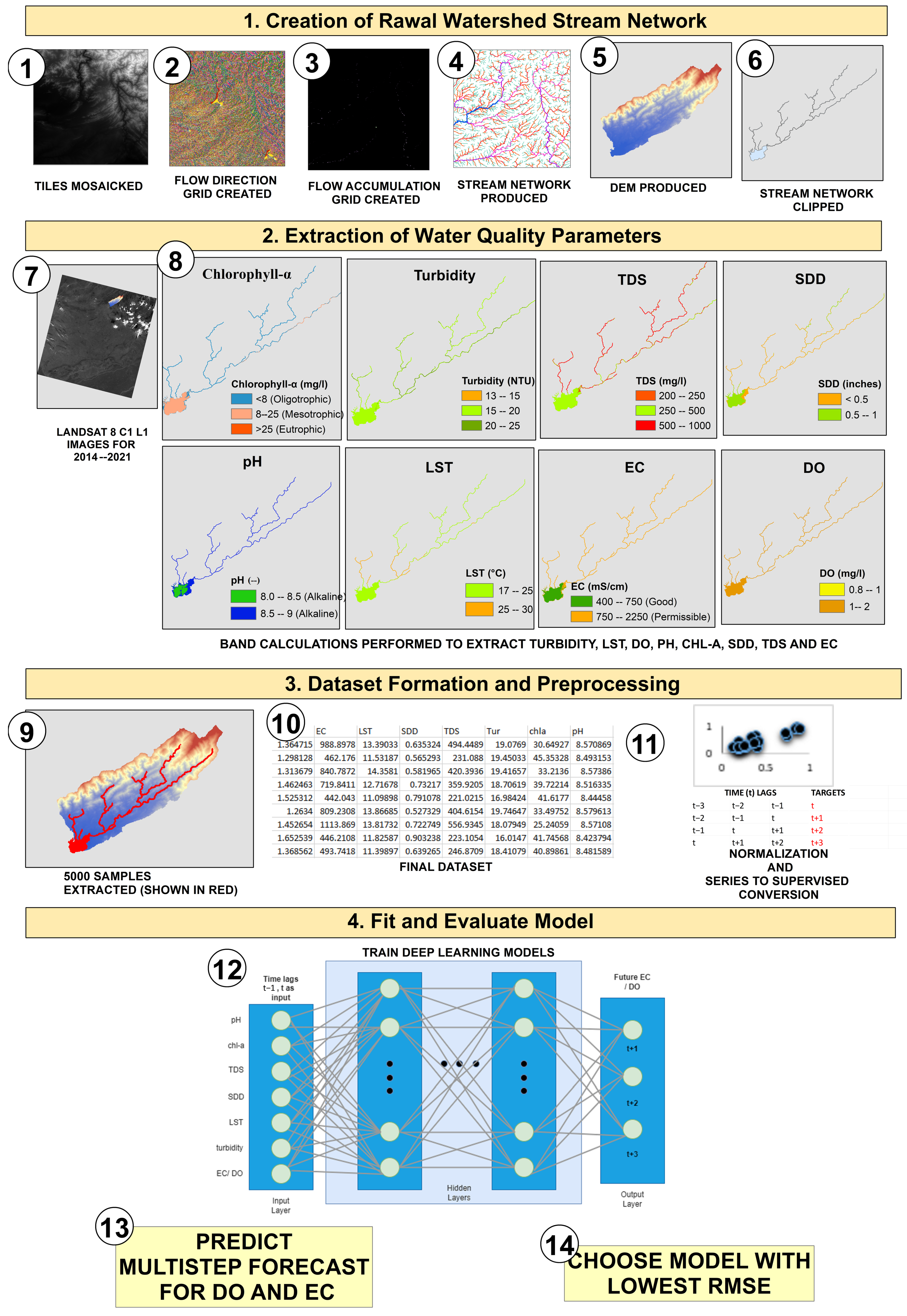
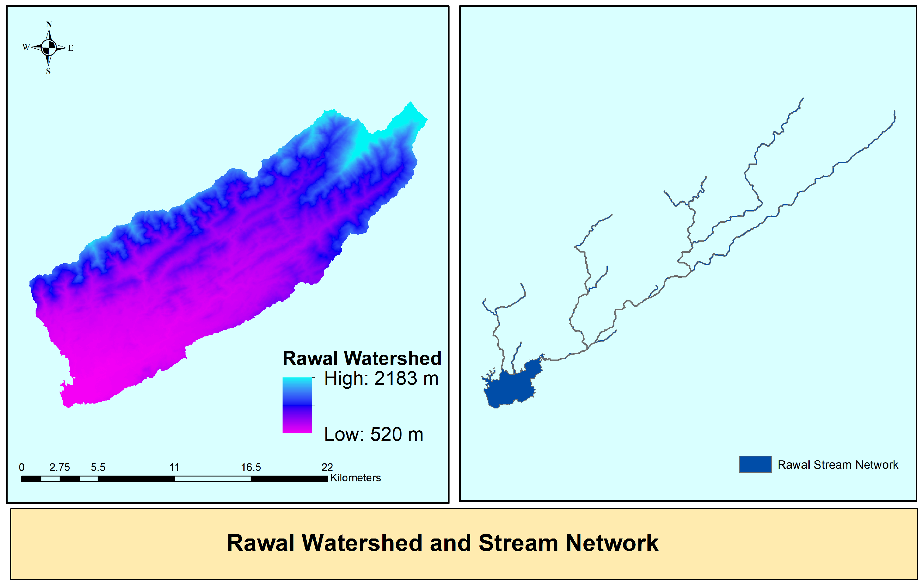
• The extraction of the stream network for the Rawal watershed from the SRTM DEM.
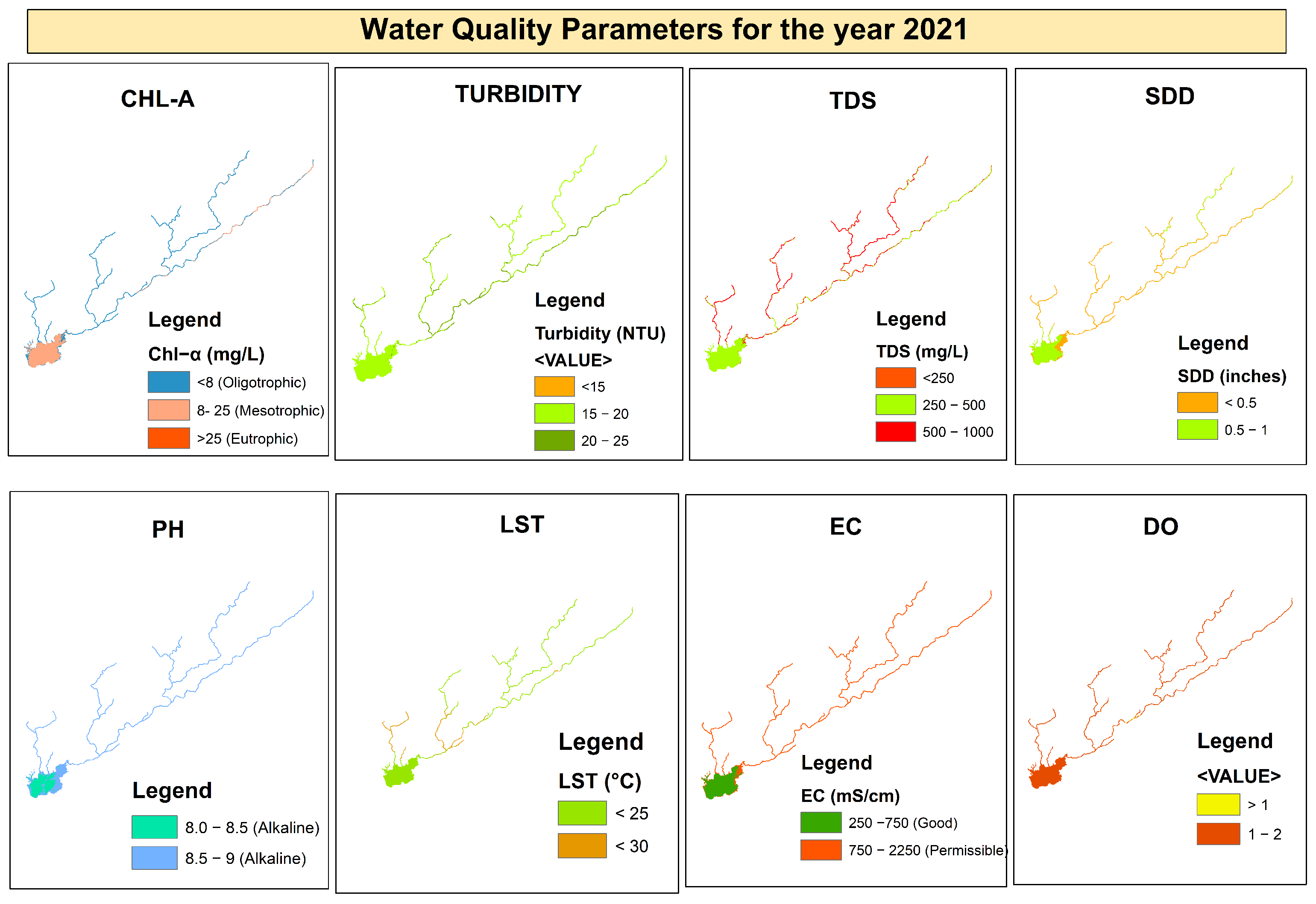
• The extraction of a total of eight water quality parameters, six optically active and two optically inactive water quality parameters, by applying estimated band equations on Landsat 8 satellite imagery for the Rawal watershed stream network pertaining to the years 2014–2021.
• The application of deep learning models for current and future multi–step forecasting of an optically active parameter, i.e., EC, and an optically inactive parameter, i.e., DO, using optically active/inactive water quality parameters. The analysis conducted using the deep learning models demonstrated the decline in water quality over the eight–year period and revealed that the factors that have contributed to the deterioration in water quality include seasonal variations and other environmental variables.

The value of using a remote sensing and machine learning approach was that it led to some important conclusions, including the identification of (i) the fact that the quality of water declined over the eight–year period, as well as (ii) the factors that contributed to this deterioration in water quality. In this study we aimed to find practical methods to analyze the factors affecting the water quality and to investigate the changes needed in the traditional water quality monitoring techniques for the betterment of society on a global scale. This will improve the socio–economic environment, which is dependent on an appropriate standard of water quality for its development, which may include activities such as agricultural operations. Therefore, the proposed solution can be used as a guideline for applications in other drinking water reservoirs besides the current study area. The hybrid deep learning and remote sensing approach can promote innovation in state–of–the–art water quality management and assessment techniques.

The paper is organized as follows. Section 2 covers the proposed methodology for the extraction of the optically active and inactive water quality parameters and the application of deep learning models is discussed. The results of the deep learning models are elaborated in Section 3. In Section 4, the conclusions and future works in this area of research are presented.

2. Materials and Methods

In this paper, we introduces a multi–step forecasting–based deep learning model for the multi–step parameter estimation of two optically active and inactive water quality parameters, i.e., EC and DO, for the study area of the Rawal watershed stream network. Figure 1 illustrates the methodology employed for creating the desired model. The process is divided into four main steps. These steps and the respective methods used are discussed in this section.

2.1. Study Area

The Rawal watershed covers an area of 272 sq km within longitudes 73°03′–73°24′ E and latitudes 33°41′–33°54′ N [42]. The watershed area is surrounded by highly populated places, which results in water quality deterioration due to anthropogenic activities such as improper sewage disposal. Water is received from 4 major streams and 43 small streams. The Rawal watershed encompasses land, as well as the water tributaries. Thus, to extract the parameter values from only the water bodies, the study area was enhanced by producing a stream network using SRTM DEM data, and this can be seen in Figure 2.

Stream Network: The production of the stream network required the latest map of the Rawal watershed area. However, due to construction and development over the years, the most recent map of the watershed did not show a high–resolution image of the area of the water streams. To overcome this issue, GIS tools were utilized to extract only the water bodies from the Rawal watershed. The resultant stream network was produced using the SRTM data. The SRTM images of the desired area were mosaicked together using ArcGIS software [43]. Later, flow direction and flow accumulation were calculated with the Hydrology toolset in ArcGIS software to produce the required DEM. This tool helped to model the flow of water across the Rawal DEM. The Rawal stream network can be seen in Figure 2.

2.2. Data Acquisition

The data were acquired in the form of multi–spectral satellite images from Landsat 8 (C1 L1) satellite data from the archives of the United States Geological Survey (USGS) [44]. The Landsat images were observed for the years 2014 to 2021, which comprised of a total of 327 images. However, in the data preprocessing phase, 167 out of 327 satellite images were found to show or cover the Rawal lake area. These preprocessed satellite images were used to perform band calculations to acquire water quality parameters from only the water streams located in the watershed. A stream network was produced using SRTM DEM data and then both optically active and inactive parameters, including pH, turbidity, DO, TDS, EC, chl–$\alpha$, SDD and LST, were extracted. Five–thousand data/sample points were retrieved from each satellite image after the calculation of the water quality parameters, i.e., 820,848 data points in total, as seen in

Table 1. Numbers of satellite images, preprocessed images and sample points retrieved for the years 2014 to 2021.

Years	No. of Images	Preprocessed Images that Cover Rawal Lake	No. of Samples
2014	41	22	107,492
2015	42	21	102,606
2016	44	23	112,378
2017	45	23	112,378
2018	42	21	102,606
2019	43	22	107,492
2020	38	19	92,834
2021	32	16	83,062
Total	327	167	820,848

.

Figure 3 shows the acquisition process for a single Landsat image and the features extracted for a single data point. Each parameter selected for this study plays a key role in the monitoring of the water health [45]. For example, the LST parameter is responsible for many water–borne processes. Similarly, high and low values of pH determine the usability of water. pH values in the range of 6.5 to 8 are considered ideal for the productivity of fish and other aquatic organisms. EC is an important indicator of pollution or some other discharge in the water body. On the other hand, the turbidity and SDD parameters signify the clarity of water, which can determine the depth of photosynthesis that can take place in the water body. Thus, aquatic organisms are dependent on water turbidity for survival as highly turbid water can impact the level of DO, which will affect the growth rate. The Chl–$\alpha$ parameter indicates the presence of algae growth, which is essential for photosynthesis and oxygen production. Another important parameter is DO, which has the highest significance amongst the other variables, as all respiring organisms are dependent on it for their survival. Moreover, the Landsat 8 remote sensor, used to retrieve data on these water quality parameters, has a spatial resolution of 15–100 m, with the presence of 11 bands. The parameters that were successfully retrieved based on the band calculations used in previous studies include the pH, turbidity, DO, TDS, EC, chl–$\alpha$, SDD and LST. These eight parameters were then reproduced for the selected study area.

Water Quality Parameter Extraction from Landsat Images

Landsat 8 (C1 L1) satellite data for an eight year time period, i.e., 2014 to 2021, were used to extract the optically active and inactive water quality features, using different band combinations. These satellite images have 11 bands with high–quality Landsat scenes, i.e., 30 m (Bands 1–7, 9), 100 m (Bands 10, 11), and 15 m (Band 8). A total of 167 images were retrieved and 5000 samples were extracted from the stream network for each image. To extract each water quality feature from the images, an estimation algorithm was applied, which involved the following steps.

• Conversion of Digital Numbers (DN) to Top–Of–Atmosphere (TOA) Reflectance:
  Preprocessing of the satellite images comprised operations including atmospheric or geometric correction and normalization. The first step of retrieving the water quality features involved the conversion of the DNs or the pixels in the satellite image to TOA reflectance values. TOA reflectance values include factors from clouds, atmospheric aerosols and gases. These DNs are converted to ToA reflectance values using rescaling coefficients and parameters found in the metadata file provided with the data and using the following expression:

  $$R_x=M_P\ast Q_{cal}+A_p$$

  (1)
  In Equation (1), $R_x$ = TOA reflectance for band number x; $M_P$ = REFLECTANCE_MULT_BAND_x, $Q_{cal}$ = standard pixels of band x or DN of band x; and $A_P$ = REFLECTANCE_ADD_BAND_x where x is band 2, 3, 4, 5 and 6, respectively. This conversion formula uses values such as REFLECTANCE_MULT_BAND and REFLECTANCE_ADD_BAND, which are kept in the metadata set with each image. REFLECTANCE_MULT_BAND is multiplied for the reflectance correction valueto be applied with each input band and its default value for Landsat 8 is 0.00002. Similarly, the REFLECTANCE_ADD_BAND is the addictive correction value for reflectance to be applied with each input band and its default value is −0.1 [46].
• Application of the Estimated Equations:
  The optically active/inactive features were then calculated by applying the algorithms given in

  Table 2. Calculations performed to determine pH, Turbidity, DO, TDS, EC, Chl–$\alpha$, SDD, and LST using Landsat 8 images.

  Parameters	Adapted Equation	Equation No	Reference
  pH	$8.790$ + ($1.141$ × $R_6$) − ($0.288$ × (($R_3$)/($R_4$)))	2	[47]
  Turbidity	$35.121$− ($14.489$ × ($R_3$/$R_4$)) − ($0.911$ × $R_5$)	3	[48]
  DO	($R_2$) / ($R_4$)	4	[31,49]
  TDS	$120.750$ + $264.752$ × ($R_5$/$R_1$)	5	[47]
  EC	$241.500$ + $529.504$ × ($R_5$/$R_1$)	6	[47]
  chl–$\alpha$	$54.658$ + $520.451$ × $R_2$ − $1221.89$ × $R_3$ + $611.115$ × $R_4$ − $198.199$ × $R_5$	7	[26]
  SDD	$0.2$ + $1.4$ × ln($R_2$/$R_4$)	8	[50]
  LST	$L_{10\Lambda }$ = $M_L$ × $Q_{cal}$ + $A_L$ 1	9	[51]
  	$BT$ = $K_2$/ln⁡ (1 + $K_1$/$L_{10\Lambda }$) 2	10
  	NDVI = (NIR − VIS)/(NIR + VIS) 3	11
  	$P_v$ = ((NDVI − $NDV{I}_{MIN}$)/($NDV{I}_{MAX}$ − $NDV{I}_{MIN}$)) ${}^2$	12
  	$ϵ$ = $0.004$ × $P_v$ + $0.986$	13
  	LST = BT/ (1 + ($\Lambda$ × BT/$\rho$) × (ln (⁡$ϵ$))) − $273.15$ 4	14

  Note(s): ¹ Here, $L_{10\Lambda }$ = TOA spectral radiance for Band 10, $M_L$ = RADIANCE_MULT_BAND_10, $A_L$ = RADIANCE_ADD_BAND_10, ² $K_1$ = K1_CONSTANT_BAND_10, $K_2$ = K2_CONSTANT_BAND_10, ³ NIR = Band 5, VIS = Band 4, ⁴ Λ = 10.895 μm, ρ = 1.438 × 10⁻² m·K.

  . These methods were selected as they performed the best amongst others for the selected study area. Band math analysis was applied to the images using the Google Earth Engine. A total of 0.82 M sample points for every feature were extracted.
  Each feature was calculated based on different band combinations. The optically inactive pH feature used a combination of bands 3, 4 and 6. The optically active turbidity feature was extracted with bands 3, 4 and 5. Bands 1 and 5 were used to extract EC and TDS. A combination of bands 2 and 4 were used to extract DO and SDD. Finally, bands 2, 3, 4 and 5 were used to retrieve chl–$\alpha$.
• Evaluation of the Equation:
  The methods were evaluated by comparing them with the observed ground parameters for the study area. The best–performing method on the selected study area was selected for extracting the sample points.

2.3. Deep Learning Models

In this study, various deep learning models, including MLP, CNN, FCN, RNN, and five variants of LSTMs, were considered for the comparison of their estimations of the water quality parameter concentrations. For time series problems, deep learning models such as RNN and LSTM can discover dependence in the historical data with the patterns in their networks. Deep networks such as CNN are used for image and video classification problems but they can also be used for sequential data. In the following, we introduce the parameters and the structures of the deep learning models used in this study.

2.3.1. Multi–Layer Perceptron (MLP)

In this study, the MLP model was made up of three layers in a dense layer. The first layer had 128 neurons and the second layer had 64 neurons, each followed by a rectified linear unit (ReLU). The ReLU activation function was used as it is fast, simple and works well with a deep neural network, compared to other activation functions. The second layer was followed by a dropout activation function. To avoid overfitting/ underfitting problems, the deep neural network used a regulatory layer known as the dropout layer [52]. The optimization hyperparameter was used to minimize the loss function to an acceptable level.

2.3.2. Convolutional Neural Network (CNN)

A one–dimensional CNN was employed for estimating water parameter concentrations in this study, and this did not differ much from a regular CNN model [53,54] other than the fact that the convolutional hidden layer operated on one–dimensional sequential data [55]. In this study, the first convolutional layer was followed by a second layer and then a pooling layer that summarized the features by filtering the output of the preceding convolutional layers. The convolutional and pooling layers were followed by a flatten layer to reduce the input to a single one–dimensional vector. Then a dense fully connected layer was implemented to interpret the extracted features.

2.3.3. Fully Connected Network (FCN)

The FCN model employed for this study was the same as the architecture originally proposed by Wang et al. in 2017 [56], composed of three convolutional blocks, in which each convolution is followed by a batch normalization fed to a ReLU activation function with a slight change in the pooling layer where instead of taking the average, the results are fed to a max pooling layer. Finally, this is followed by a dense layer to obtain the final output.

2.3.4. Recurrent Neural Network (RNN)

The RNN employed in this study for predicting multi–step water quality parameter concentrations is known as the stacked RNN. It uses a combination of multiple recurrent neural networks [57]. The model had 2 layers; the first RNN layer was followed by a dropout layer and then the second RNN layer, followed by the final dense layer.

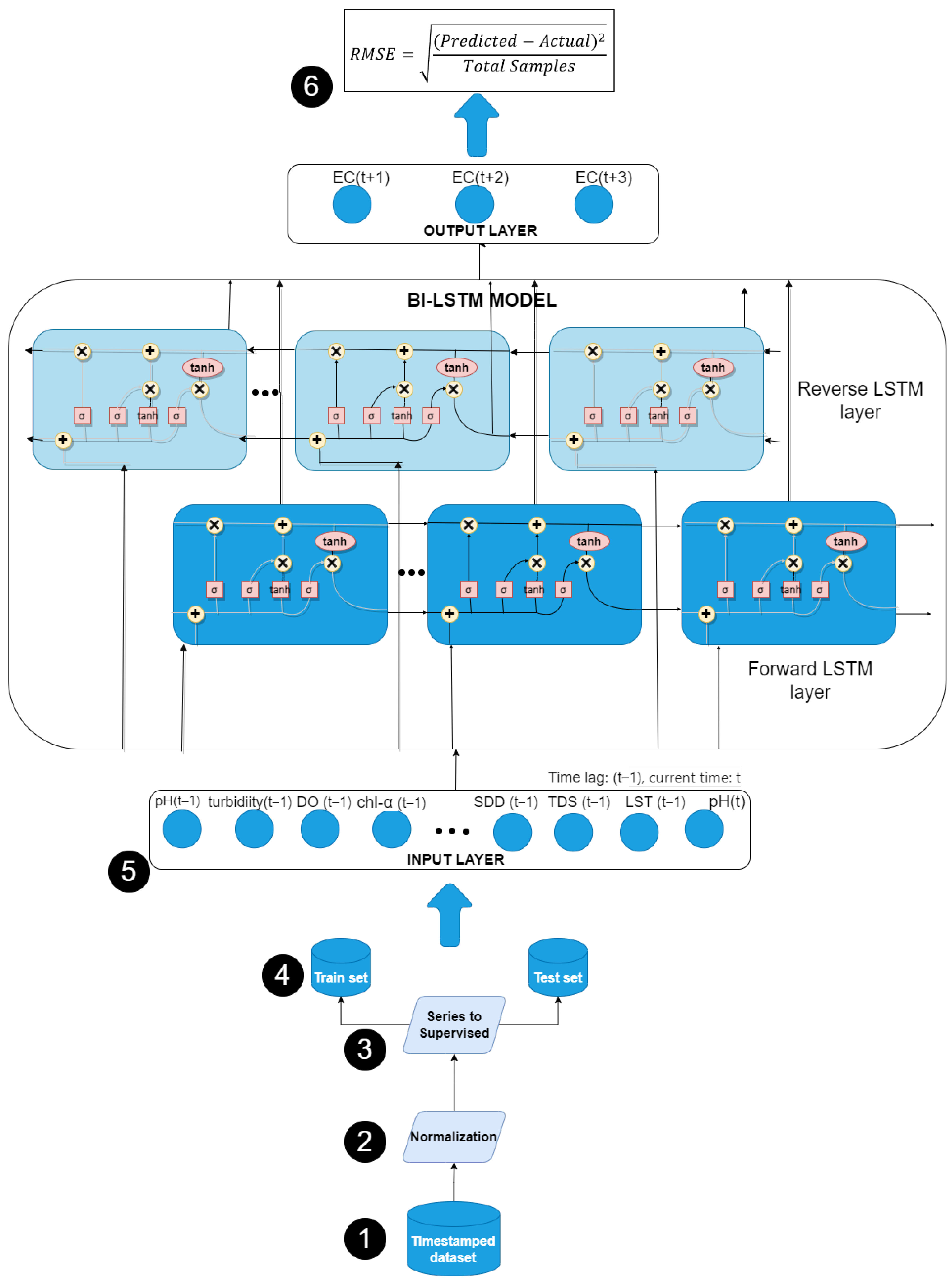
2.3.5. Long Short Term Memory (LSTM) and Its Variants

LSTM was first proposed by Hochreiter and Schmidhubercin 1997 [58], and it is popular due to its internal self–looped cell that captures the dynamic characteristics of a time series problem. Five variants of LSTM models were evaluated in this study. These included the basic LSTM and the LSTM–dominated and LSTM–integrated variations. The integrated variations consisted of LSTM cells with other components, whereas the dominated variations focused only on the performance of the LSTM cells [41]. The LSTM–dominated versions included a stacked LSTM (S–LSTM), a bidirectional LSTM (Bi–LSTM), a convolutional LSTM (Conv–LSTM), and an LSTM–integrated variant, i.e., a CNN LSTM (CNN–LSTM). These variants were chosen for their distinct characteristics in handling regression and time series problems.

Vanilla LSTM (V–LSTM) is the most commonly used LSTM proposed by Graves and Schmidhuber. It has a single hidden layer with forget gates and an output layer. S–LSTM is simply an LSTM model that has multiple hidden layers, each stacked one on top of another. All layers use the output of the previous layer as their input. The final output is passed on to a full–connect layer for classification. Bi–LSTM learns both forwards and backwards, as proposed in [59]. This model is capable of accessing long–range context in both directions. The model is trained using back–propagation through time (BPTT) [60]. The Conv–LSTM model has units that directly read the convolutional input. Conv–LSTM tends to preserve spatial information, which can help in the reconstruction of data. CNN–LSTM is a hybrid of the CNN model with an LSTM backend. This hybrid model uses a CNN to interpret subsequences of input and passes them together to the LSTM model to interpret. Each input is passed through a convolutional and max pooling layer.

2.3.6. Training of the Deep Learning Model

Once the water quality features were extracted from the clipped Rawal stream network, the data were then prepped for the multi–step forecasting problem. This step involved data preprocessing and normalization, before outputting datafor the training of the deep model. The procedure is described below.

• Data Preparation: The dataset was converted into a time series dataset by transforming the timestamp column as an index.
• Normalization: All features in the dataset were normalized in the range of 0 to 1, in a process referred to as min–max normalization. For every water quality feature, the values were in different units. For example, the pH of water was mostly in the range of 6 to 9. Similarly, the EC of water lay in the range of 400 µS/cm to 1000 µS/cm. Thus, to bring uniformity into the dataset, the values were normalized for each feature in the range of 0 to 1.
• Series to Supervised: The dataset was then further transformed for a supervised learning problem by splitting the input sequence, i.e., the input data at the current time (t) were split into a three dimensional shape (samples, time steps, features) for a multiple input multi–step time series, where a lag time (t − n) and further time steps (t + 1, t + 2, …, t + n) were defined for features (n).
• Training and test sets: The transformed dataset was then split into training and test sets. Here, the last 2 years’ worth of data (220,845 samples) were selected as the test set and 5 years’ worth of data (600,000 samples) were selected as the training set.
• Model Parameters: The parameters (neurons, epochs, and hidden layers) of the deep model were initialized. Here, each deep model had a different set of parameters with a difference in dropout layers and hidden layers.
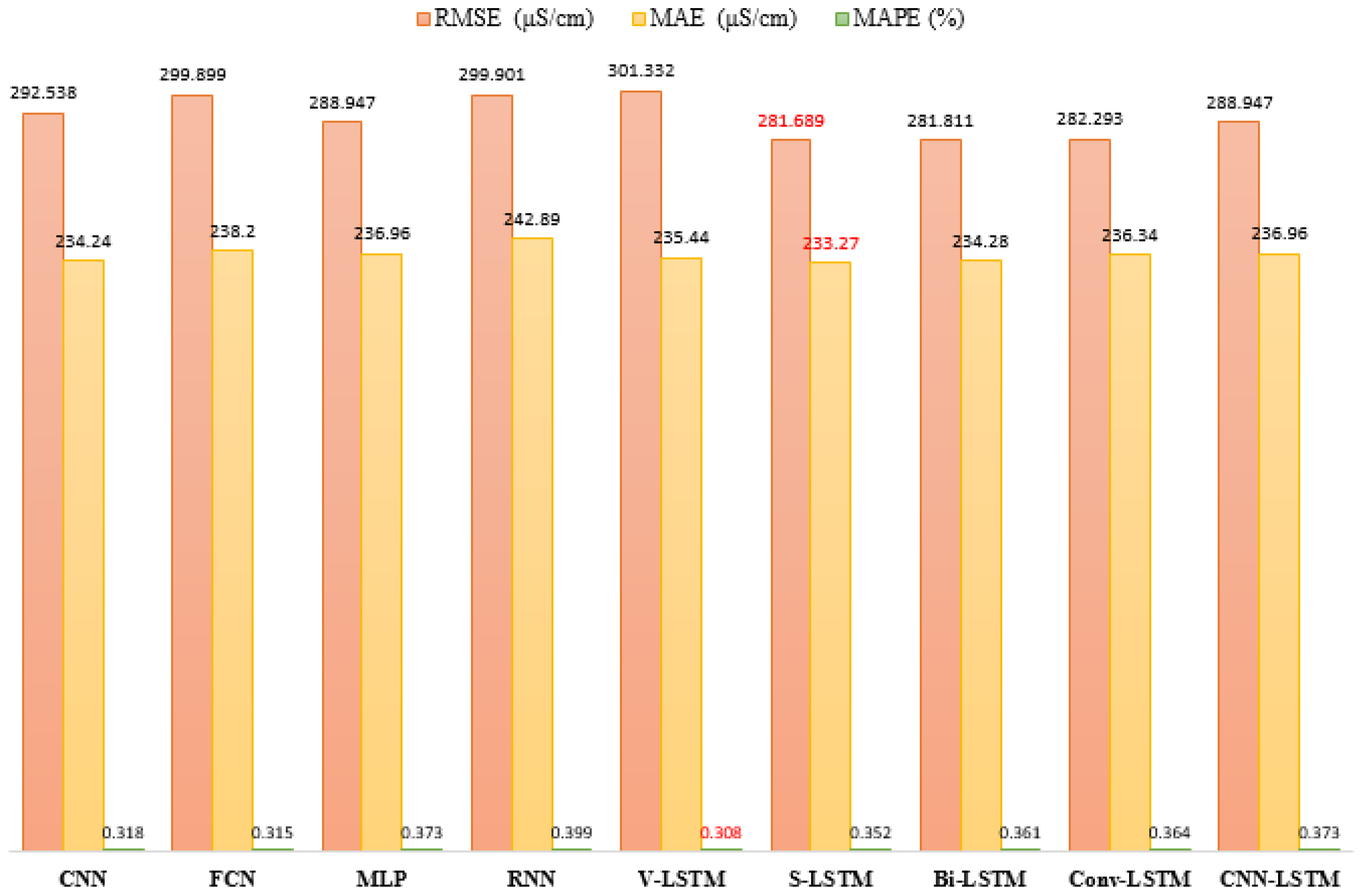
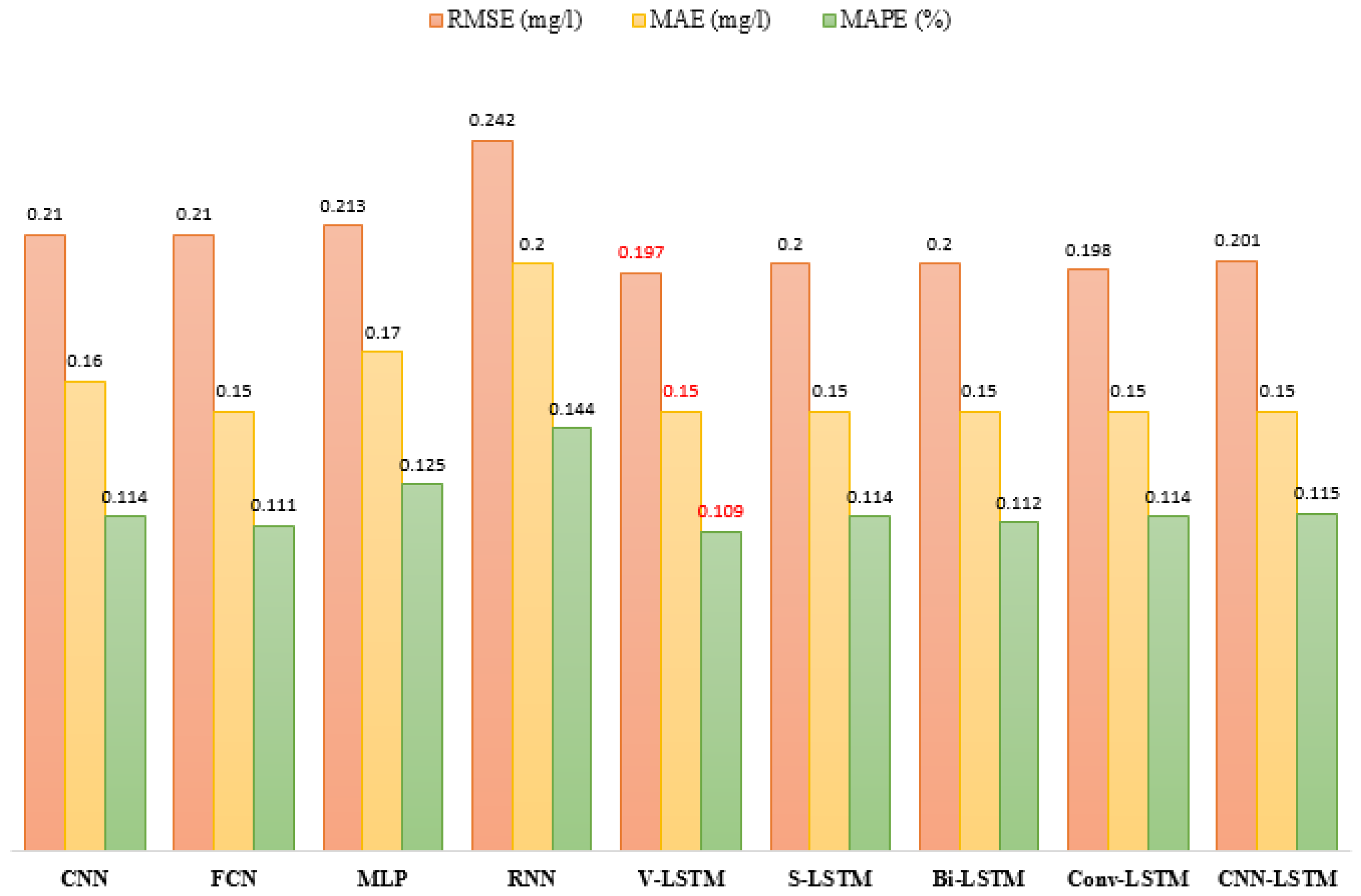
• Model Evaluation: The model was evaluated based on the three loss functions, i.e., root mean square error (RMSE), mean absolute error (MAE), and mean absolute percentage error (MAPE). RMSE and MAE give the error in the same units as the predicted variable and MAPE is given as a percentage (%).

Figure 4 shows the designed Bi–LSTM architecture used for predicting the multi–step EC concentrations. This figure demonstrates the six steps involved in the training of the deep model, as mentioned in detail in Section 2.3.6.

3. Results and Discussion

The aim of this study was to explore the use of different deep learning models in current and multi–step parameter estimation for both optically active and inactive water quality parameters, i.e., EC and DO. The results and findings are discussed in detail in this section. The models were assessed in terms of three loss functions i.e., the root mean square error (RMSE), mean absolute error (MAE) and the mean absolute percentage error (MAPE). The RMSE and MAE both measure the error in the same units as the predicted variable. On the other hand, the MAPE indicates the error margin in the model forecast and is expressed as a percentage (%). Moreover, there are some temporal dependencies for time series forecasting problems. To overcome such dependencies, the data were trained by determining a split point without shuffling them. Hence, the training was performed on 0.6M samples without shuffling the data. A sample of the features calculated from the Landsat 8 images for the year 2021 is depicted in Figure 5 and the last twenty samples are shown in

Table 3. Last 20 water quality samples extracted from LANDSAT 8 images for September 2021.

DO	EC	LST	SDD	TDS	Tur	chl–$\mathit{\alpha }$	pH
1.69	487.22	23.71	0.94	243.61	15.51	31.23	8.43
1.69	466.66	23.14	0.94	233.33	15.73	32.73	8.43
1.58	524.88	23.78	0.84	262.44	15.76	24.90	8.44
1.37	698.71	23.78	0.64	349.36	18.71	26.96	8.53
1.41	713.33	24.06	0.68	356.66	17.18	14.78	8.52
1.52	492.27	23.50	0.79	246.14	16.45	28.01	8.45
1.54	488.48	23.43	0.80	244.24	16.14	26.70	8.44
1.35	824.81	22.26	0.62	412.41	18.32	13.58	8.56
1.52	496.10	23.49	0.78	248.05	16.35	26.80	8.45
1.47	1065.93	23.72	0.74	532.96	17.32	1.79	8.57
1.66	460.37	23.40	0.91	230.19	15.63	31.76	8.43
1.60	526.96	23.23	0.86	263.48	16.27	28.01	8.45
1.64	493.14	23.08	0.90	246.57	16.27	31.84	8.45
1.25	1105.11	23.61	0.51	552.56	18.69	−9.95	8.69
1.69	468.18	23.62	0.93	234.09	15.72	33.26	8.43
1.28	685.49	18.29	0.54	342.75	19.07	1.93	8.59
1.49	773.22	24.09	0.76	386.61	17.18	16.71	8.51
1.50	993.48	22.87	0.77	496.74	16.65	0.72	8.53
1.76	456.41	23.55	0.99	228.20	15.46	35.63	8.42

. The results of the deep learning algorithms—the CNN, FCN, RNN, MLP and LSTM variants—are assessed and each model performance is compared on the basis of the lowest RMSE reached with the same number of epochs.

The regression time series problem was framed inthe following two formulations:

• Predict the DO and EC at the current time event (t) given the eight water quality features at the prior time steps, that is, a lag time period of three (t − 3, t − 2, t − 1).
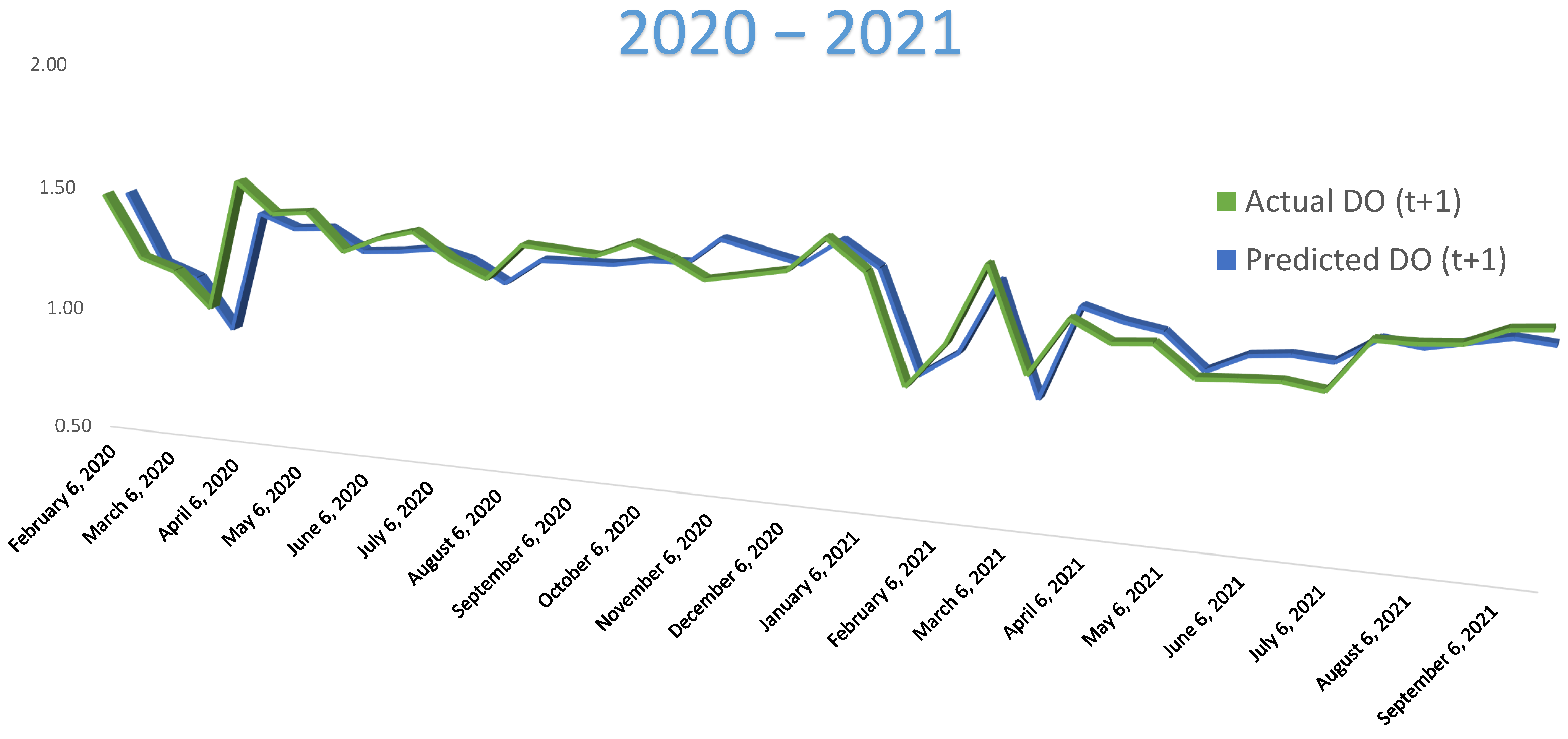
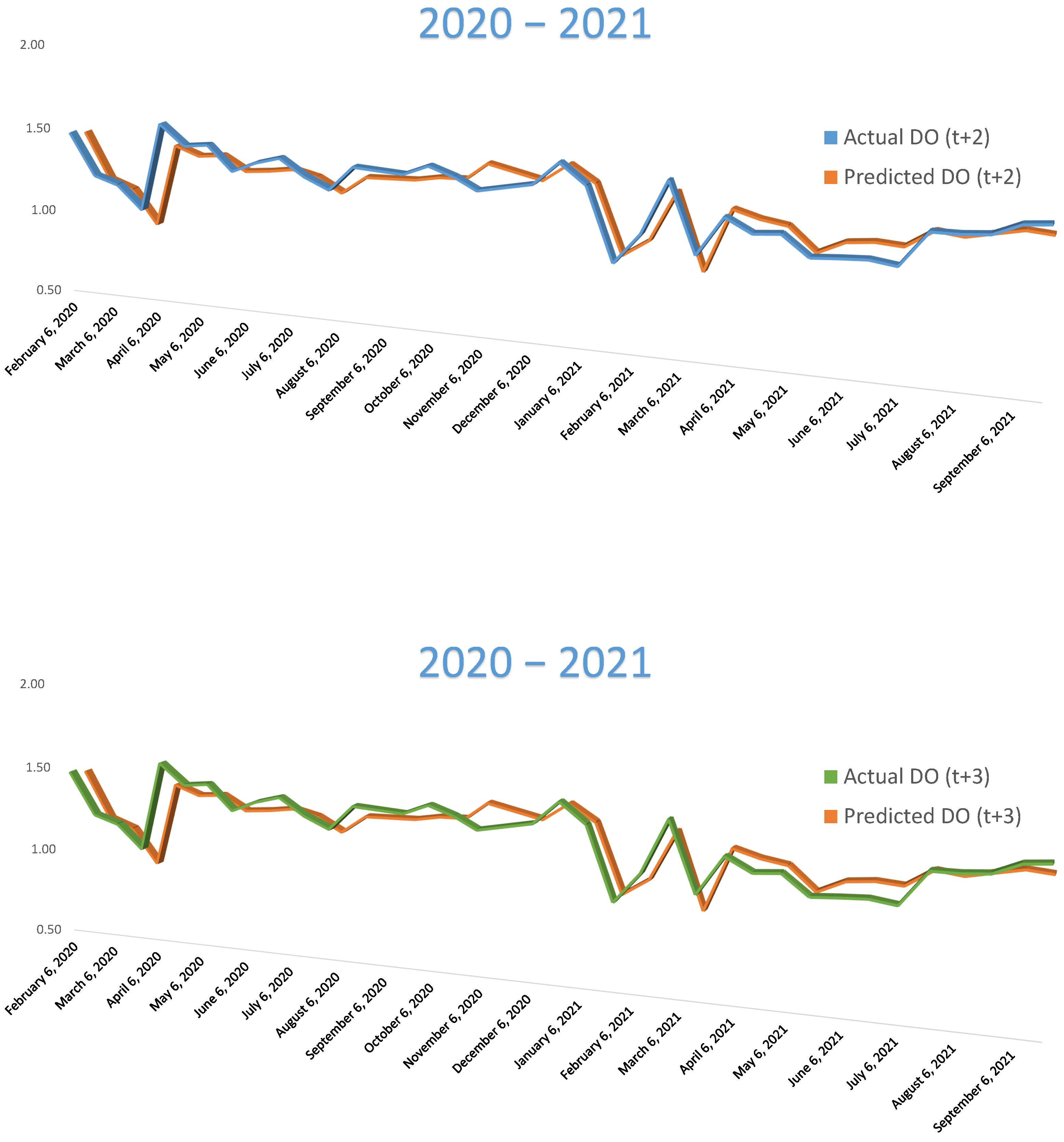
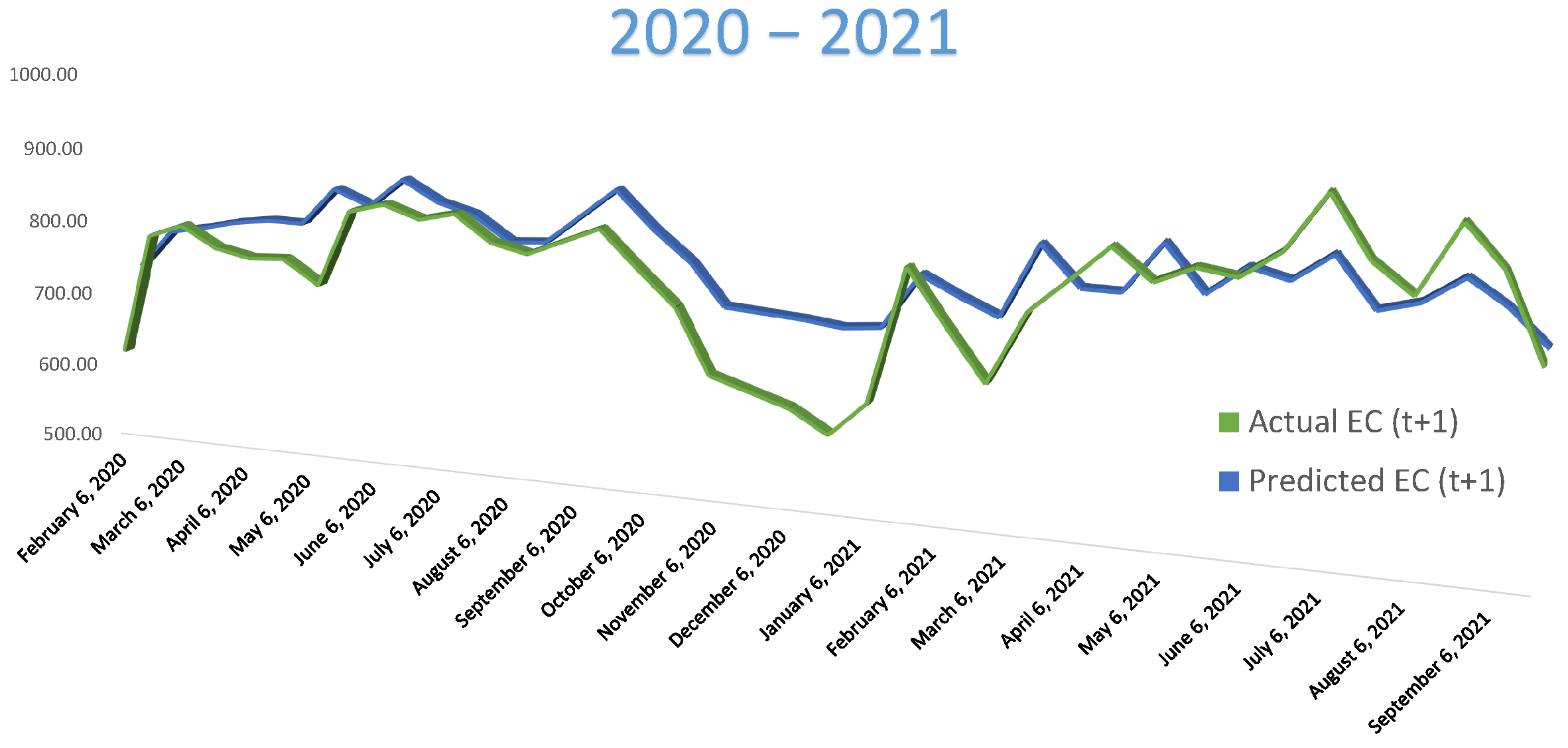
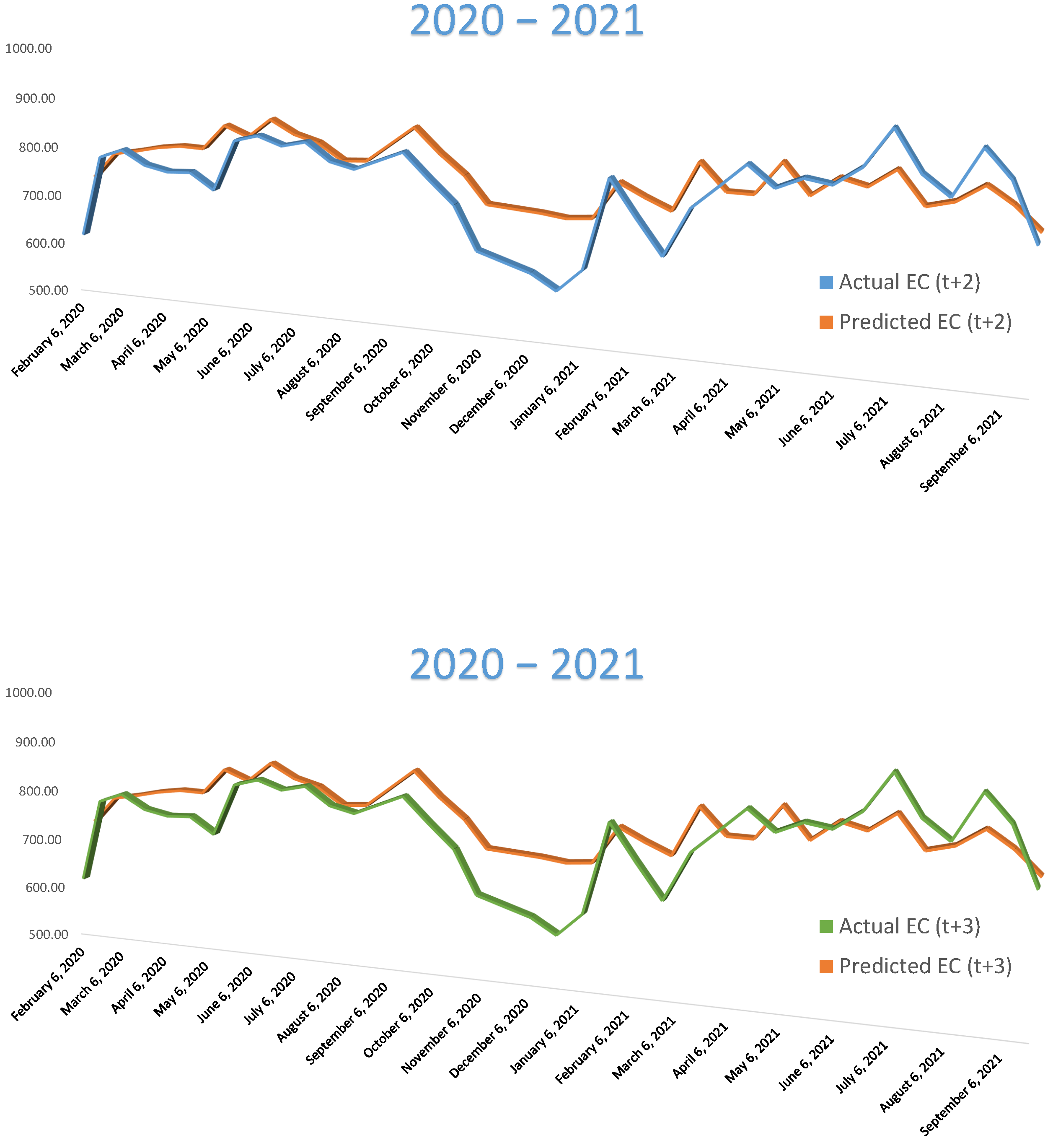
• Predict the DO and EC for the next three events (t + 1, t + 2, t + 3) based on the eight water quality features at the prior time steps with a lag time period of one (t − 1).

Next, the results for both of these formulations are discussed. The LSTM variants showed exemplary performance as compared to the other deep learning models.

Predictions of current event parameters: For current predictions of the optically active and inactive parameters, the last three lag events (t − 3, t − 2, t − 1) were used to predict the current time event (t). Figure 6 displays the results for the current EC predictions. It can be seen that S–LSTM outperformed the other deep models, followed by the bi–LSTM with RMSE values of 281.689 and 281.811 (µS/cm), respectively. Overall, the LSTM variants displayed a much better performance for the current time event prediction task. This shows that the LSTM–dominated variants outperformed the LSTM–integrated ones. On the other hand, FCN and RNN models exhibited high RMSE values up to 301 (µS/cm). Figure 7 displays the results for the current DO prediction task. The best results were achieved with V–LSTM and conv–LSTM, with RMSE values of 0.197, 0.198 (mg/L), respectively. Here, the LSTM variants showed a better performance when compared with other deep models, with V–LSTM giving only an 0.109 % MAPE. Similarly, for DO prediction, the RNN model demonstrated a high RMSE of 0.242 (mg/L).

Predictions of future event parameters: For multi–step forecasts, a lag time period of one (t − 1) was used to predict the next three events, i.e., t + 1, t + 2, and t + 3. For the future time event predictions of optically active and inactive parameters, EC and DO, Bi–LSTM performed the best among the other LSTM variants. For DO, V–LSTM and Bi–LSTM showed the minimum RMSE values of 0.2 and 0.199 (mg/L), respectively. Other variants, such as CNN–LSTM and Conv–LSTM, showed much better results than other deep models for the multi–step forecasting of DO, as shown in

Table 4. Results for the optically inactive parameter DO for the multi–step (t + 1, t + 2, t + 3) events.

Deep Learner	Lag Time Period	Time Steps	Epochs	Hyperparameters	RMSE (mg/L)	MAE (mg/L)	MAPE (%)
CNN	1	3	500	filters = 6, 12, average pooling (size 1)	0.213	0.16	0.116
FCN	1	3	500	filters = 128, 256, 128, kernel = 1, 1, 1, max pooling (size 1)	0.209	0.15	0.1121
MLP	1	3	500	128, 64 with dropout	0.212	0.16	0.115
RNN	1	3	500	20 neurons, 2 layers with 1 dropout 0.2, 8 dense layer	0.238	0.18	0.135
V–LSTM	1	3	500	50 neurons	0.22	0.153	0.111
S–LSTM	1	3	500	dropout = 0.2, 4 layers with 50 neurons	0.213	0.16	0.116
Bi–LSTM	1	3	500	50 neurons	0.1994	0.15	0.114
Conv–LSTM	1	3	500	filters = 64, kernel = 1, LSTM with 50 neurons	0.203	0.15	0.114
CNN–LSTM	1	3	500	filters = 64 and 128, kernel = 1, max pooling, LSTM with 50 neurons	0.206	0.16	0.116

Note(s): ¹ The lowest MAPE retrieved. ² The second lowest RMSE retrieved. ³ The lowest MAE retrieved. ⁴ The lowest RMSE retrieved.

. The RNN model exhibited a high RMSE of 0.238 (mg/L). For EC, the best results were shown by the two variants of LSTM as well, i.e., S–LSTM and Bi–LSTM with RMSE values of 281.93 and 281.741 (µS/cm), respectively, as seen in

Table 5. Results for the optically active parameter EC for the multi–step (t + 1, t + 2, t + 3) events.

Deep Learner	Lag Time Period	Time Steps	Epochs	Hyperparameters	RMSE (µS/cm)	MAE (µS/cm)	MAPE (%)
CNN	1	3	500	filters = 64, 128, average pooling (size 1)	294.38	238.72	0.33
FCN	1	3	500	filters = 128, 256, 128, kernel = 1, 1, 1, max pooling (size 1)	296.464	238.59	0.3251
MLP	1	3	500	128, 64 with dropout	288.939	236.96	0.373
RNN	1	3	500	20 neurons, 2 layers with 1 dropout 0.2, 8 dense layer	288.613	238.73	0.386
V–LSTM	1	3	500	50 neurons	290.254	234.232	0.326
S–LSTM	1	3	500	dropout = 0.2, 4 layers with 50 neurons	281.933	234.99	0.361
Bi–LSTM	1	3	500	50 neurons	281.7414	234.36	0.363
Conv–LSTM	1	3	500	filters = 64, kernel = 1, LSTM with 50 neurons	282.153	235.55	0.359
CNN–LSTM	1	3	500	filters = 64 and 128, kernel = 1,max pooling, LSTM with 50 neurons	282.614	236.25	0.360

Note(s): ¹ The lowest MAPE retrieved. ² The lowest MAE retrieved. ³ The second lowest RMSE retrieved. ⁴ The lowest RMSE retrieved.

. Thus, for both current and future water quality forecasts, the LSTM variants showed much better results than the other deep models. However, Bi–LSTM was the best performer when compared with the other LSTM variants. For EC, FCN and CNN showed high RMSE values of 296.46 and 294.38 (µS/cm), respectively.

Figure 8 and Figure 9 show a year–wise comparison of the Bi–LSTM model for DO and EC, respectively. The performance of the Bi–LSTM model was the best among the deep learning models. The actual and predicted forecasts for both DO and EC parameters for the years 2020 and 2021 can be seen. Figure 8 shows that, for each time step, the error margin for the DO predictions was very low. However, for EC, the forecasts for October through December 2020 were not that accurate as seen in Figure 9. This could be due to the fact that EC shows variations during the summer and winter seasons. EC values in winter are generally lower than those in the summer season due to the high evaporation losses in summer and the increased drainage water inflow [61]. Moreover, the year–wise analysis showed a decline in the water quality over the eight–year period, as we can observe a decline in the observed concentrations of the EC and DO water quality variables. The decline in concentrations over the years can be attributed to seasonal variations and other environmental variables [62].

4. Conclusions

Rawal Lake is the main source of drinking water for the residents of Islamabad and Rawalpindi. However, the lake water is unfit to drink from as it receives untreated sewage and other wastewater due to the increase in population. Water quality assessments are made using manual labor and in laboratories, which is time-consuming. Thus, using the advancements in remote sensing and other technologies, water quality monitoring tasks can be made simple and robust. In this study, eight water quality features for the years 2014 to 2021 were calculated using Landsat 8 images of the study area of the Rawal stream network that were extracted with SRTM DEM data, using hydrological GIS tools. Six optically active water quality parameters, including turbidity, Chl– $\alpha$, SDD, TDS, EC, and LST, and two optically inactive features, i.e., DO and pH, were taken as inputs to observe the water quality parameter estimations for current and future events.

The experiments were limited to predicting only one of the active and inactive water quality parameters, i.e., EC and DO. The multi–step water quality forecasts were made using different deep learning models, i.e., CNN, FCN, MLP, RNN, and five variants of the LSTM model, which included LSTM–dominated and LSTM–integrated versions, including vanilla, stacked, bi–directional, convolutional, and a CNN LSTM hybrid. These models were then compared on the basis of the lowest RMSE achieved. The results showed that the LSTM variants displayed the best performance in the current and future multi–step parameter estimations for both optically active and inactive parameters with the bi–directional LSTM emerging as the leading variant among them. Moreover, the performance of the LSTM–dominated variants was better when compared with the LSTM–integrated version for the observed problem.

The proposed approach, using the combination of remote sensing and machine learning, identified that the water quality declined over the eight–year period, as observed through the concentrations of the water quality variables. Moreover, the factors that contributed to this water quality deterioration include the concentrations of water quality variables that are affected by seasonal variations and other environmental variables. Thus, in the future, some additional water quality parameters can be used for multi–step water quality parameter estimations and forecasts. These environmental variables, which may include air quality parameters, slope, soil type, and the geology and lithology of the study area, can be considered to examine water quality parameters.

References

1. Hamzaoui-Azaza, F.; Ketata, M.; Bouhlila, R.; Gueddari, M.; Riberio, L. Hydrogeochemical characteristics and assessment of drinking water quality in Zeuss–Koutine aquifer, southeastern Tunisia. Environ. Monit. Assess. 2011, 174, 283–298. [Google Scholar] [CrossRef] [PubMed]
2. Pazand, K.; Hezarkhani, A.; Ghanbari, Y.; Aghavali, N. Groundwater geochemistry in the Meshkinshahr basin of Ardabil province in Iran. Environ. Earth Sci. 2012, 65, 871–879. [Google Scholar] [CrossRef]
3. Issaka, S.; Ashraf, M.A. Impact of soil erosion and degradation on water quality: A review. Geol. Ecol. Landscapes 2017, 1, 1–11. [Google Scholar] [CrossRef] [Green Version]
4. Qadir, A.; Malik, R.N.; Husain, S.Z. Spatio-temporal variations in water quality of Nullah Aik-tributary of the river Chenab, Pakistan. Environ. Monit. Assess. 2008, 140, 43–59. [Google Scholar] [CrossRef]
5. Nazeer, S.; Hashmi, M.Z.; Malik, R.N. Heavy metals distribution, risk assessment and water quality characterization by water quality index of the River Soan, Pakistan. Ecol. Indic. 2014, 43, 262–270. [Google Scholar] [CrossRef]
6. Bhatti, N.; Siyal, A.; Qureshi, A. Groundwater quality assessment using water quality index: A Case study of Nagarparkar, Sindh, Pakistan. Sindh Univ. Res.-J.-Surj. (Sci. Ser.) 2018, 50, 227–234. [Google Scholar]
7. Chen, L.; Tan, C.H.; Kao, S.J.; Wang, T.S. Improvement of remote monitoring on water quality in a subtropical reservoir by incorporating grammatical evolution with parallel genetic algorithms into satellite imagery. Water Res. 2008, 42, 296–306. [Google Scholar] [CrossRef]
8. Hsu, H.H.; Chen, L.; Kou, C.H.; Yeh, H.C.; Wang, T.S. Applying Multi-temporal Satellite Imageries to Estimate Chlorophyll-a Concentration in Feitsui Reservoir Using ANNs. In Proceedings of the 2009 International Joint Conference on Artificial Intelligence, Hainan, China, 25–26 April 2009; IEEE Computer Society: Los Alamitos, CA, USA, 2009; pp. 345–348. [Google Scholar]
9. Wen, X.P.; Yang, X.F. Monitoring of water quality using remote sensing techniques. Appl. Mech. Mater. 2010, 29, 2360–2364. [Google Scholar] [CrossRef]
10. Fichot, C.G.; Downing, B.D.; Bergamaschi, B.A.; Windham-Myers, L.; Marvin-DiPasquale, M.; Thompson, D.R.; Gierach, M.M. High-resolution remote sensing of water quality in the San Francisco Bay–Delta Estuary. Environ. Sci. Technol. 2016, 50, 573–583. [Google Scholar] [CrossRef]
11. Ritchie, J.C.; Zimba, P.V.; Everitt, J.H. Remote sensing techniques to assess water quality. Photogramm. Eng. Remote Sens. 2003, 69, 695–704. [Google Scholar] [CrossRef] [Green Version]
12. Kallio, K. Remote sensing as a tool for monitoring lake water quality. Hydrol. Limnol. Asp. Lake Monit. 2000, 14, 237. [Google Scholar]
13. Ahmed, M.; Mumtaz, R.; Baig, S.; Zaidi, S.M.H. Assessment of correlation amongst physico-chemical, topographical, geological, lithological and soil type parameters for measuring water quality of Rawal watershed using remote sensing. Water Supply 2022, 22, 3645–3660. [Google Scholar] [CrossRef]
14. Ahmed, M.; Mumtaz, R.; Hassan Zaidi, S.M. Analysis of water quality indices and machine learning techniques for rating water pollution: A case study of Rawal Dam, Pakistan. Water Supply 2021, 21, 3225–3250. [Google Scholar] [CrossRef]
15. Xiang, L.; Li, J.; Hu, A.; Zhang, Y. Deterministic and probabilistic multi-step forecasting for short-term wind speed based on secondary decomposition and a deep learning method. Energy Convers. Manag. 2020, 220, 113098. [Google Scholar] [CrossRef]
16. Yan, K.; Wang, X.; Du, Y.; Jin, N.; Huang, H.; Zhou, H. Multi-step short-term power consumption forecasting with a hybrid deep learning strategy. Energies 2018, 11, 3089. [Google Scholar] [CrossRef] [Green Version]
17. Jayasinghe, W.L.P.; Deo, R.C.; Ghahramani, A.; Ghimire, S.; Raj, N. Deep Multi-Stage Reference Evapotranspiration Forecasting Model: Multivariate Empirical Mode Decomposition Integrated With the Boruta-Random Forest Algorithm. IEEE Access 2021, 9, 166695–166708. [Google Scholar] [CrossRef]
18. Lv, Z.; Xu, J.; Zheng, K.; Yin, H.; Zhao, P.; Zhou, X. Lc-rnn: A deep learning model for traffic speed prediction. In Proceedings of the 27th International Joint Conference on Artificial Intelligence (IJCAI-18), Stockholm, Sweden, 13–19 July 2018; Volume 2018, p. 27. [Google Scholar]
19. Bloemheuvel, S.; Hoogen, J.v.d.; Jozinović, D.; Michelini, A.; Atzmueller, M. Multivariate Time Series Regression with Graph Neural Networks. arXiv 2022, arXiv:2201.00818. [Google Scholar]
20. Dumas, J.; Cointe, C.; Fettweis, X.; Cornélusse, B. Deep learning-based multi-output quantile forecasting of PV generation. In Proceedings of the 2021 IEEE Madrid PowerTech, Madrid, Spain, 28 June–2 July 2021; IEEE: Piscataway, NJ, USA, 2021; pp. 1–6. [Google Scholar]
21. Gitelson, A.A.; Merzlyak, M.N. Remote sensing of chlorophyll concentration in higher plant leaves. Adv. Space Res. 1998, 22, 689–692. [Google Scholar] [CrossRef]
22. Xu, M.; Liu, H.; Beck, R.; Lekki, J.; Yang, B.; Shu, S.; Liu, Y.; Benko, T.; Anderson, R.; Tokars, R.; et al. Regionally and locally adaptive models for retrieving chlorophyll-a concentration in inland waters from remotely sensed multispectral and hyperspectral imagery. IEEE Trans. Geosci. Remote Sens. 2019, 57, 4758–4774. [Google Scholar] [CrossRef]
23. Harrington, J.A., Jr.; Schiebe, F.R.; Nix, J.F. Remote sensing of Lake Chicot, Arkansas: Monitoring suspended sediments, turbidity, and Secchi depth with Landsat MSS data. Remote Sens. Environ. 1992, 39, 15–27. [Google Scholar] [CrossRef]
24. Imen, S.; Chang, N.B.; Yang, Y.J. Developing the remote sensing-based early warning system for monitoring TSS concentrations in Lake Mead. J. Environ. Manag. 2015, 160, 73–89. [Google Scholar] [CrossRef]
25. Sharaf El Din, E. A novel approach for surface water quality modelling based on Landsat-8 tasselled cap transformation. Int. J. Remote Sens. 2020, 41, 7186–7201. [Google Scholar] [CrossRef]
26. Lim, J.; Choi, M. Assessment of water quality based on Landsat 8 operational land imager associated with human activities in Korea. Environ. Monit. Assess. 2015, 187, 1–17. [Google Scholar] [CrossRef] [PubMed]
27. Kapalanga, T.S. Assessment and Development of Remote Sensing Based Algorithms for Water Quality Monitoring in Olushandja Dam, North-Central Namibia. Master’s Thesis, University of Zimbabwe, Harare, Zimbabwe, 2015. [Google Scholar]
28. Liu, H.; Xu, M.; Beck, R. An Ensemble Approach to Retrieving Water Quality Parameters from Multispectral Satellite Imagery. In Proceedings of the IGARSS 2018-2018 IEEE International Geoscience and Remote Sensing Symposium, Valencia, Spain, 22–27 July 2018; IEEE: Piscataway, NJ, USA, 2018; pp. 9284–9287. [Google Scholar]
29. Wang, J.; Shi, T.; Yu, D.; Teng, D.; Ge, X.; Zhang, Z.; Yang, X.; Wang, H.; Wu, G. Ensemble machine-learning-based framework for estimating total nitrogen concentration in water using drone-borne hyperspectral imagery of emergent plants: A case study in an arid oasis, NW China. Environ. Pollut. 2020, 266, 115412. [Google Scholar] [CrossRef] [PubMed]
30. El Din, E.S.; Zhang, Y. Estimation of both optical and nonoptical surface water quality parameters using Landsat 8 OLI imagery and statistical techniques. J. Appl. Remote Sens. 2017, 11, 046008. [Google Scholar]
31. Theologou, I.; Patelaki, M.; Karantzalos, K. Can single empirical algorithms accurately predict inland shallow water quality status from high resolution, multi-sensor, multi-temporal satellite data? Int. Arch. Photogramm. Remote Sens. Spat. Inf. Sci. 2015, 40, 1511. [Google Scholar] [CrossRef] [Green Version]
32. Tan, G.; Yan, J.; Gao, C.; Yang, S. Prediction of water quality time series data based on least squares support vector machine. Procedia Eng. 2012, 31, 1194–1199. [Google Scholar] [CrossRef] [Green Version]
33. Najafzadeh, M.; Homaei, F.; Farhadi, H. Reliability assessment of water quality index based on guidelines of national sanitation foundation in natural streams: Integration of remote sensing and data-driven models. Artif. Intell. Rev. 2021, 54, 4619–4651. [Google Scholar] [CrossRef]
34. Vakili, T.; Amanollahi, J. Determination of optically inactive water quality variables using Landsat 8 data: A case study in Geshlagh reservoir affected by agricultural land use. J. Clean. Prod. 2020, 247, 119134. [Google Scholar] [CrossRef]
35. Najafzadeh, M.; Ghaemi, A.; Emamgholizadeh, S. Prediction of water quality parameters using evolutionary computing-based formulations. Int. J. Environ. Sci. Technol. 2019, 16, 6377–6396. [Google Scholar] [CrossRef]
36. Miikkulainen, R.; Liang, J.; Meyerson, E.; Rawal, A.; Fink, D.; Francon, O.; Raju, B.; Shahrzad, H.; Navruzyan, A.; Duffy, N.; et al. Evolving deep neural networks. In Artificial Intelligence in the Age of Neural Networks and Brain Computing; Elsevier: Cambridge, MA, USA, 2019; pp. 293–312. [Google Scholar]
37. Pyo, J.C.; Ligaray, M.; Kwon, Y.S.; Ahn, M.H.; Kim, K.; Lee, H.; Kang, T.; Cho, S.B.; Park, Y.; Cho, K.H. High-spatial resolution monitoring of phycocyanin and chlorophyll-a using airborne hyperspectral imagery. Remote Sens. 2018, 10, 1180. [Google Scholar] [CrossRef] [Green Version]
38. Niu, C.; Tan, K.; Jia, X.; Wang, X. Deep learning based regression for optically inactive inland water quality parameter estimation using airborne hyperspectral imagery. Environ. Pollut. 2021, 286, 117534. [Google Scholar] [CrossRef] [PubMed]
39. Faruk, D.Ö. A hybrid neural network and ARIMA model for water quality time series prediction. Eng. Appl. Artif. Intell. 2010, 23, 586–594. [Google Scholar] [CrossRef]
40. Zhang, L.; Ma, X.; Shi, P.; Bi, S.; Wang, C. Regcnn: A deep multi-output regression method for wastewater treatment. In Proceedings of the 2019 IEEE 31st International Conference on Tools with Artificial Intelligence (ICTAI), Portland, OR, USA, 4–6 November 2019; IEEE: Piscataway, NJ, USA, 2019; pp. 816–823. [Google Scholar]
41. Yu, Y.; Si, X.; Hu, C.; Zhang, J. A review of recurrent neural networks: LSTM cells and network architectures. Neural Comput. 2019, 31, 1235–1270. [Google Scholar] [CrossRef] [PubMed]
42. Ashraf, A. Chapter: Changing Hydrology of the Himalayan Watershed. 2013. Available online: https://www.intechopen.com/chapters/43184 (accessed on 13 May 2022).
43. ArcGIS Pro. Available online: https://www.esri.com/en-us/arcgis/products/arcgis-pro/overview (accessed on 13 May 2022).
44. Survey, U.U.G. Earthexplorer. Available online: https://earthexplorer.usgs.gov/ (accessed on 13 May 2022).
45. Gorde, S.; Jadhav, M. Assessment of water quality parameters: A review. J. Eng. Res. Appl. 2013, 3, 2029–2035. [Google Scholar]
46. Paul, B. Estimation of Greenfield Changes in Kerala using NDVI on Landsat Data. Pramana Res. J. 2019, 9, 757–770. [Google Scholar]
47. Abdullah, H.S. Water Quality Assessment for Dokan Lake Using Landsat 8 Oli Satellite Images. Master’s Thesis, University of Sulaimani, Sulaymaniyah, Iraq, 2015. [Google Scholar]
48. Khattab, M.F.; Merkel, B.J. Application of Landsat 5 and Landsat 7 images data for water quality mapping in Mosul Dam Lake, Northern Iraq. Arab. J. Geosci. 2014, 7, 3557–3573. [Google Scholar] [CrossRef]
49. Khalil, M.T.; Saad, A.; Ahmed, M.; El Kafrawy, S.B.; Emam, W.W. Integrated field study, remote sensing and GIS approach for assessing and monitoring some chemical water quality parameters in Bardawil lagoon, Egypt. Int. J. Innov. Res. Sci. Eng. Technol. 2016, 5, 10–15680. [Google Scholar]
50. Deutsch, E.; Alameddine, I.; El-Fadel, M. Developing Landsat Based Algorithms to Augment in Situ Monitoring of Freshwater Lakes and Reservoirs. In Proceedings of the 11th International Conference on Hydroinformatics, New York, NY, USA, 17–21 August 2014; City University of New York (CUNY): New York, NY, USA, 2014; Volume 1. [Google Scholar]
51. Avdan, U.; Jovanovska, G. Algorithm for automated mapping of land surface temperature using LANDSAT 8 satellite data. J. Sens. 2016, 2016, 1480307. [Google Scholar] [CrossRef] [Green Version]
52. Srivastava, N.; Hinton, G.; Krizhevsky, A.; Sutskever, I.; Salakhutdinov, R. Dropout: A simple way to prevent neural networks from overfitting. J. Mach. Learn. Res. 2014, 15, 1929–1958. [Google Scholar]
53. Szegedy, C.; Liu, W.; Jia, Y.; Sermanet, P.; Reed, S.; Anguelov, D.; Erhan, D.; Vanhoucke, V.; Rabinovich, A. Going deeper with convolutions. In Proceedings of the IEEE Conference on Computer Vision and Pattern Recognition, Boston, MA, USA, 7–12 June 2015; pp. 1–9. [Google Scholar]
54. Krizhevsky, A.; Sutskever, I.; Hinton, G.E. Imagenet classification with deep convolutional neural networks. Adv. Neural Inf. Process. Syst. 2012, 25. [Google Scholar] [CrossRef]
55. Zhao, B.; Lu, H.; Chen, S.; Liu, J.; Wu, D. Convolutional neural networks for time series classification. J. Syst. Eng. Electron. 2017, 28, 162–169. [Google Scholar] [CrossRef]
56. Wang, Z.; Yan, W.; Oates, T. Time series classification from scratch with deep neural networks: A strong baseline. In Proceedings of the 2017 International Joint Conference on Neural Networks (IJCNN), Anchorage, AK, USA, 14–19 May 2017; IEEE: Piscataway, NJ, USA, 2017; pp. 1578–1585. [Google Scholar]
57. Medsker, L.R.; Jain, L. Recurrent neural networks. Des. Appl. 2001, 5, 64–67. [Google Scholar]
58. Hochreiter, S.; Schmidhuber, J. Long short-term memory. Neural Comput. 1997, 9, 1735–1780. [Google Scholar] [CrossRef]
59. Graves, A.; Jaitly, N.; Mohamed, A.r. Hybrid speech recognition with deep bidirectional LSTM. In Proceedings of the 2013 IEEE Workshop on Automatic Speech Recognition and Understanding, Olomouc, Czech Republic, 8–12 December 2013; IEEE: Piscataway, NJ, USA, 2013; pp. 273–278. [Google Scholar]
60. Boden, M. A guide to recurrent neural networks and backpropagation. Dallas Proj. 2002, 2, 1–10. [Google Scholar]
61. Sallam, G.A.; Elsayed, E. Estimating the impact of air temperature and relative humidity change on the water quality of Lake Manzala, Egypt. J. Nat. Resour. Dev. 2015, 5, 76–87. [Google Scholar] [CrossRef] [Green Version]
62. Gray, N.F. Drinking Water Quality: Problems and Solutions, 2nd ed.; Cambridge University Press: Cambridge, UK, 2008. [Google Scholar]
Figure 1. Steps proposed for estimating multi–step forecasts of EC and DO parameters for the study area of the Rawal watershed.
Water 14 02112 g001
Figure 2. Study area DEM of the Rawal watershed and the stream network extracted after processing.
Water 14 02112 g002
Figure 3. Data acquisition process for a single mosaicked Landsat image.
Water 14 02112 g003
Figure 4. The architecture of the designed Bi–LSTM model, displaying the steps involved in training the deep model to predict the multi–step EC concentrations.
Water 14 02112 g004
Figure 5. Water quality features, i.e., C h l α , turbidity, TDS, SDD, pH, LST, EC, and DO, extracted from Landsat 8 images using the adapted equations mentioned in Table 2 for the year 2021.
Water 14 02112 g005
Figure 6. Results for the optically active parameter EC for the current (t) event.
Water 14 02112 g006
Figure 7. Results for the optically inactive parameter DO for the current (t) event.
Water 14 02112 g007
Figure 8. Test data results of the Bi–LSTM model for multi–step (t + 1, t + 2, t + 3) forecasts of the optically inactive parameter DO for the years 2020 and 2021.
Water 14 02112 g008aWater 14 02112 g008b
Figure 9. Test data results of Bi–LSTM model for multi–step (t + 1, t + 2, t + 3) forecasts of the optically active parameter EC for the years 2020 and 2021.
Water 14 02112 g009aWater 14 02112 g009b