Review

Measurement of Water Soil Erosion at Sparacia Experimental Area (Southern Italy): A Summary of More than Twenty Years of Scientific Activity

Department of Agricultural, Food and Forestry Sciences, University of Palermo, Viale delle Scienze, Building 4, 90128 Palermo, Italy
*
Author to whom correspondence should be addressed.
Water 2022, 14(12), 1881; https://doi.org/10.3390/w14121881
Submission received: 12 May 2022 / Revised: 6 June 2022 / Accepted: 7 June 2022 / Published: 11 June 2022
(This article belongs to the Special Issue Soil Erosion Measurement Techniques and Field Experiments)

Abstract

:
The main purpose of this article is to give a general idea of the scientific activity that was carried out starting from the 2000s on the basis of the data collected in the plots installed at the Sparacia experimental station for soil erosion measurement in Sicily, South Italy. The paper includes a presentation of the experimental site, a description of the methods and procedures for measuring soil erosion processes both available in the literature and applied at the Sparacia station (sediment sampling and water level reading in the storage tanks for total erosion measurements; profilometer, and Structure from Motion technique for rill erosion measurements), and the main results obtained in the monitoring period in the experimental site. The latter concern the effects of plot size and steepness on soil loss, the measurement variability, the frequency analysis of soil loss, the rill erosion characterization, and the comparison between rill and interrill erosion rates. Each of these topics is addressed with multi-temporal analyses performed with increasing size of the available database, which allowed to draw robust conclusions. Soil loss did not vary appreciably with plot length in contrast with the assumption made in the USLE/RUSLE. The variability of the measurements of soil loss, runoff volume, and sediment concentration at the event scale in replicated plots decreased as the mean measured value increased. The normalized event soil loss was distributed according to a two-component distribution. A power relationship between rill volumes and lengths was established. The measurements also confirmed the morphological similarity between the channels of the rills and ephemeral gullies described by a power dimensionless relationship. Rill erodibility of the sampled clay soil varied over time, maintaining relatively low values. Finally, rill erosion was dominant relative to interrill erosion, and a more efficient sediment transport system through the rill network occurred as plot steepness increased.

1. Introduction

In the research field of water soil erosion, the measurement of a representative variable of the phenomenon (e.g., plot soil loss, basin sediment yield) and its controlling factors (e.g., rainfall energetic characteristics, soil grain size distribution) allows for directly evaluating the magnitude of the phenomenon in the area of interest, extending and improving the knowledge of the erosive processes, and establishing the effectiveness of soil conservation practices. Moreover, the simulation of the erosive phenomenon by mathematical models needs measurement of the parameters and/or variables included in the equations used to describe the different subprocesses. The measurements are also necessary to calibrate and validate the models through the comparison between the estimated and measured values of the variable expressive of the erosive phenomenon.
Laboratory erosion research can be carried out in highly controlled experimental conditions and is ideal for fast and repeatable experiments, but it usually requires using scale models and disturbed soil samples whose representativeness of field conditions is rather uncertain. Instead, field erosion research allows for gaining data at the proper scale and with undisturbed soils. Moreover, field data are generally representative of the climatic, soil, morphologic, and land use characteristics of the sampled site. However, these types of data are less accurate than the laboratory ones due to the practical problems of experimental field activities. In addition, to obtain representative data of average or extreme conditions for the sampled site, a multiyear monitoring period is needed, with noticeable costs and practical problems.
This paper summarizes the scientific activity that has been going on for more than twenty years in the Sparacia experimental station for soil erosion measurement in Sicily, South Italy. The Sparacia station of the Department of Agricultural, Food, and Forest Sciences—Palermo University is located approximately 100 km south of Palermo. The climate is of Mediterranean semiarid type with an average annual rainfall of 700 mm. The soil is a Vertic Xerocrept and has a clay texture (62% clay, 33% silt, and 5% sand) and negligible gravel content. The experimental station includes 20 plots with different lengths λ, widths wi, and slope steepness s. Six plots of 22 m × 8 m (λ × wi), two plots of 33 m × 8 m, two plots of 44 m × 8 m, two plots of 11 m × 4 m, two plots of 11 m × 2 m and two plots of 22 m × 2 m are installed on a 14.9% slope (Figure 1a), where a recording rain gauge operates with a 1 min resolution. Two plots of 22 m × 6 m are established on a 22% slope, and two plots of 22 m × 6 m are established on a 26% slope (Figure 1b). Rainfall data are measured with a recording rain gauge located near the four plots at 1 min intervals. The oldest plots (four plots of 22 m × 8 m) were constructed in 1999, whereas the most recent plots (two plots of 22 m × 2 m) were constructed in 2007. Plots are maintained in cultivated fallow, with up and downhill tillage, by a power cultivator. Tillage is conducted 3–4 times per year when the soil is relatively dry.
Runoff and associated sediments are intercepted by a gutter placed at the lower end of each plot and collected into a storage system consisting of tanks of known geometric characteristics that are arranged in series (Figure 2a). Total runoff and soil loss are measured after each erosive event (i.e., an event producing measurable runoff and sediment) or after a sequence of events if they are separated by a short time interval. Microplots of 0.25 m × 0.25 m and 0.40 m × 0.40 m were also installed on the 14.9 and 22% slopes, and two experimental basins of 3.67 ha and 30 ha are also located in the experimental area. The present paper focuses only on the soil erosion measurement at the plot scale. These measurements allowed parameterizing and validating Universal Soil Loss Equation (USLE)-based models for estimating event soil loss where the runoff coefficient is included in the erosivity factor [2,3]. Among these models, the so-called USLE-MM was developed through main steps starting from 2008 [4], while the USLE-MB [5] was proposed more recently and resulted in similar estimate performances as the former.
The paper reports both the methods to measure rill, interrill erosion, and total, i.e., rill + interrill, erosion at the Sparacia station and the main results concerning the effects of plot size and steepness on soil loss, the measurement variability, the frequency analysis of soil loss, the rill erosion characterization, and the comparison between rill and interrill erosion rates. A section concerning a review on soil loss measurement is first presented.

2. A Brief Summary on Soil Loss Measurement in the Literature

The spatial scale at which the measurement is performed (splash cup, microplot, plot, hillslope, or watershed) and the applied measurement technique have to be chosen in the light of the considered erosion subprocesses (e.g., impact, interrill, rill, and gully). Field plots with different sizes and steepness are often used to measure interrill and rill erosion. Microplots, with a small surface area varying approximately between 0.04 m2 and 10 m2 [6,7], are used to measure interrill erosion because rill development is not usual. Plots approximately 10–200 m long and 2–50 m wide [8] can be used to measure total, i.e., rill + interrill, erosion. Soil erosion and runoff were recognized to be dependent on the spatial scale [9,10], which makes questionable upscaling of plot erosion measurement to the basin scale. This scale dependency is attributed to spatial variability in infiltration, temporal variations in rainfall intensity during a storm event, hillslope sediment sinks, and sediment delivery along flow paths within a basin [11] that are not generally represented at the plot scale. As a result, measured erosion rates per unit area are higher on the plot than on the basin scale. On the other hand, larger plots allow for a better representation of the hydrological and erosive response of a given ecosystem [9,12], and a plot length of 20 m is sufficient to determine runoff and sediment export rates representative of a basin [13].
The measurement of the total soil loss from the experimental plots is performed either by collecting a portion of the total surface runoff coming from a conveyance system (e.g., H-flume or pipe) [14] in a sampling unit or the whole runoff inside a storage system. In the former case, once calibrated in the field, the sampling unit directly allows for measuring runoff volume and sediment concentration (e.g., Coshocton wheel [15], Fagna-type unit [16]) or storing runoff and sediments for large runoff events (multislot divisors [8,17]). In the second case, the water–sediment mixture is usually collected into tanks of known geometry, and its volume is determined by measuring the water depth. The plot soil loss is equal to the sediment mean concentration by volume. Sediment concentration can be measured by either catching the whole sediment amount after siphoning the supernatant-cleared water or collecting a sample of the mixed suspension [18]. The good accuracy of the first technique is paid by the necessity to remove high mud volumes to oven-dry in the laboratory, which makes this technique more and more cumbersome and time-consuming as stored runoff and plots’ number and size increase. In order to obtain reliable soil loss measurements by the second technique, the sample has to be representative of the whole suspension; that is, the sampled suspended sediment concentration has to be equal to the actual one. This occurs in the case of homogeneity of the suspension, i.e., when the sample concentration in any measurement point of the tank is equal to the actual concentration. This occurrence can be hindered by the incomplete mixing of the suspension [6,19].
For instance, Lang [20] detected that sampling with a bottle at the bottom of the tank, where the soil–water mixture was vigorously agitated to suspend sediment, determined underestimations of sediment concentration ranging from −17 to −74%. Zobisch et al. [21] measured total soil loss by adding the suspended sediment stored in a large tank and the sediment settled in a smaller metal bucket placed within the tank. The suspension was stirred, and its concentration was determined on a sample taken by an immersed laboratory beaker. The dry weight of the total settled sediments was also determined. Zobisch et al. [21] verified a poor accuracy of soil loss measurement and its strong dependence on the field workers, which negatively affected the repeatability of the sampling procedure. They concluded that the differences were due to the level of mixing thoroughness of the suspended sediment and the timing and plunging depth of the sample beaker. The sampling procedure of Ciesiolka et al. [22] consisted of stirring the mixture in the tank and taking samples simultaneously at three depths. The average of three sediment concentrations was used as a representative value for the entire depth of the mixture. The measured sediment concentration systematically underestimated the actual one. The authors proposed an equation based on settling theory to remove the error due to the delay time between stirring and sampling, which reduced the underestimation to values generally ranging from −66 to −6%. The residual underestimation could be due to other sources of error, such as a not uniform sediment distribution within the tank and the sampling technique. A cylindrical sampler was used by Nikkami [23] after stirring the suspension in the storage tank to withdraw a column of suspension, and the results were compared with those obtained by bottle and pipette samplings. The latter underestimated the actual sediment concentration and were unreliable, while the measurements by the cylindrical sampler were affected by errors ranging from −18 to −4%. A similar sampling cylinder with a closing valve at the bottom was proposed by Carollo et al. [24] (Figure 3) and tested to be applied for soil loss measurement at the Sparacia experimental area. The details regarding the cylinder and the applied sampling procedure are reported below. Bagarello and Ferro [19], Bagarello et al. [6], and Todisco et al. [25] evaluated factors affecting the measured sediment concentration and derived calibration curves for the sediment storage tanks at the Sparacia and Masse (Umbria, central Italy) stations. The experimental stations are characterized by the same type of plots, runoff storage system, and different soils.

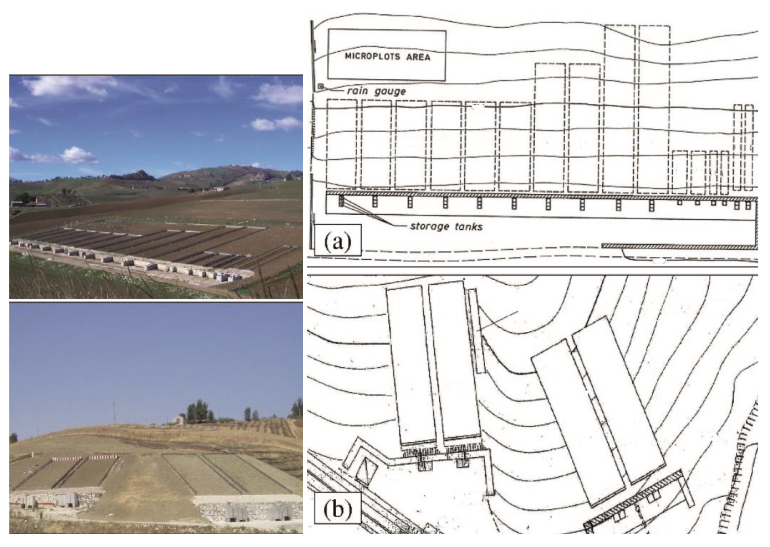
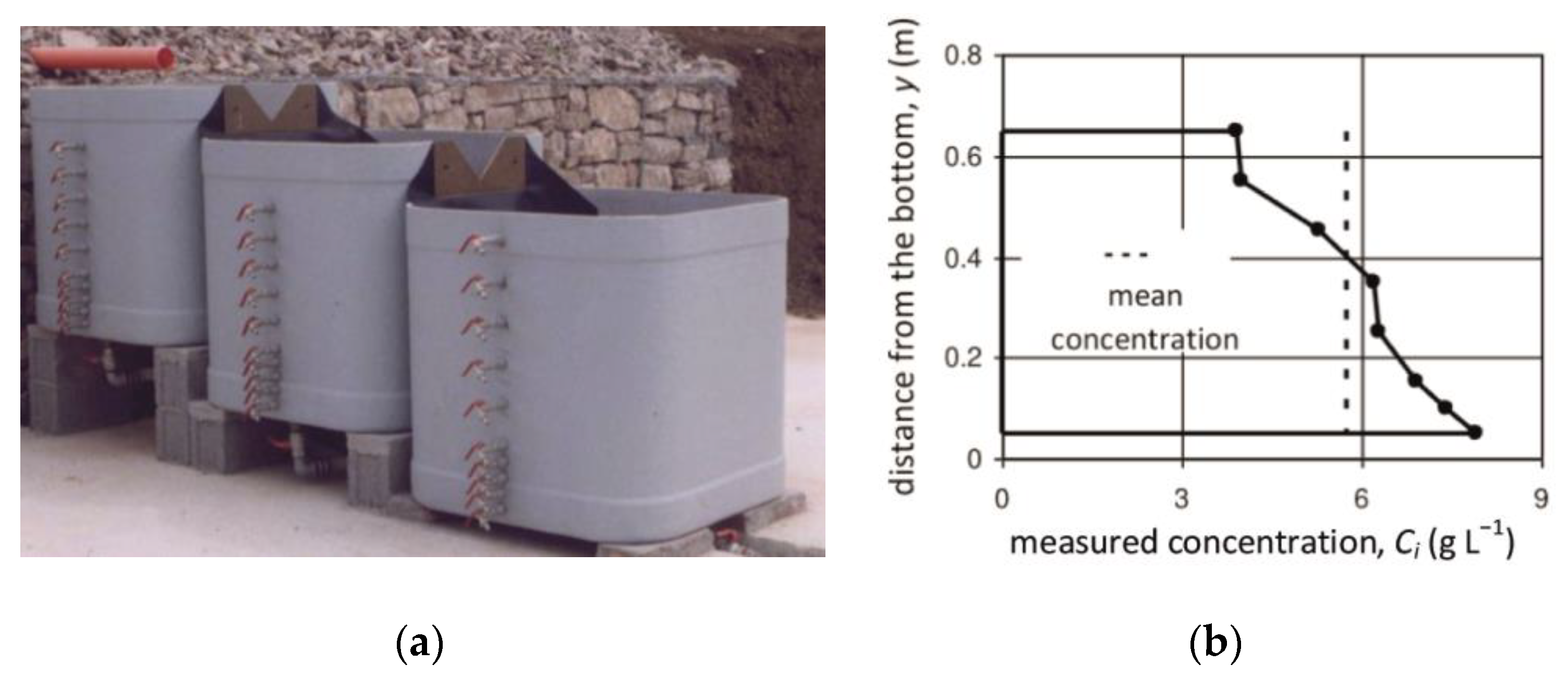
3. Measurement of Total Erosion at Sparacia

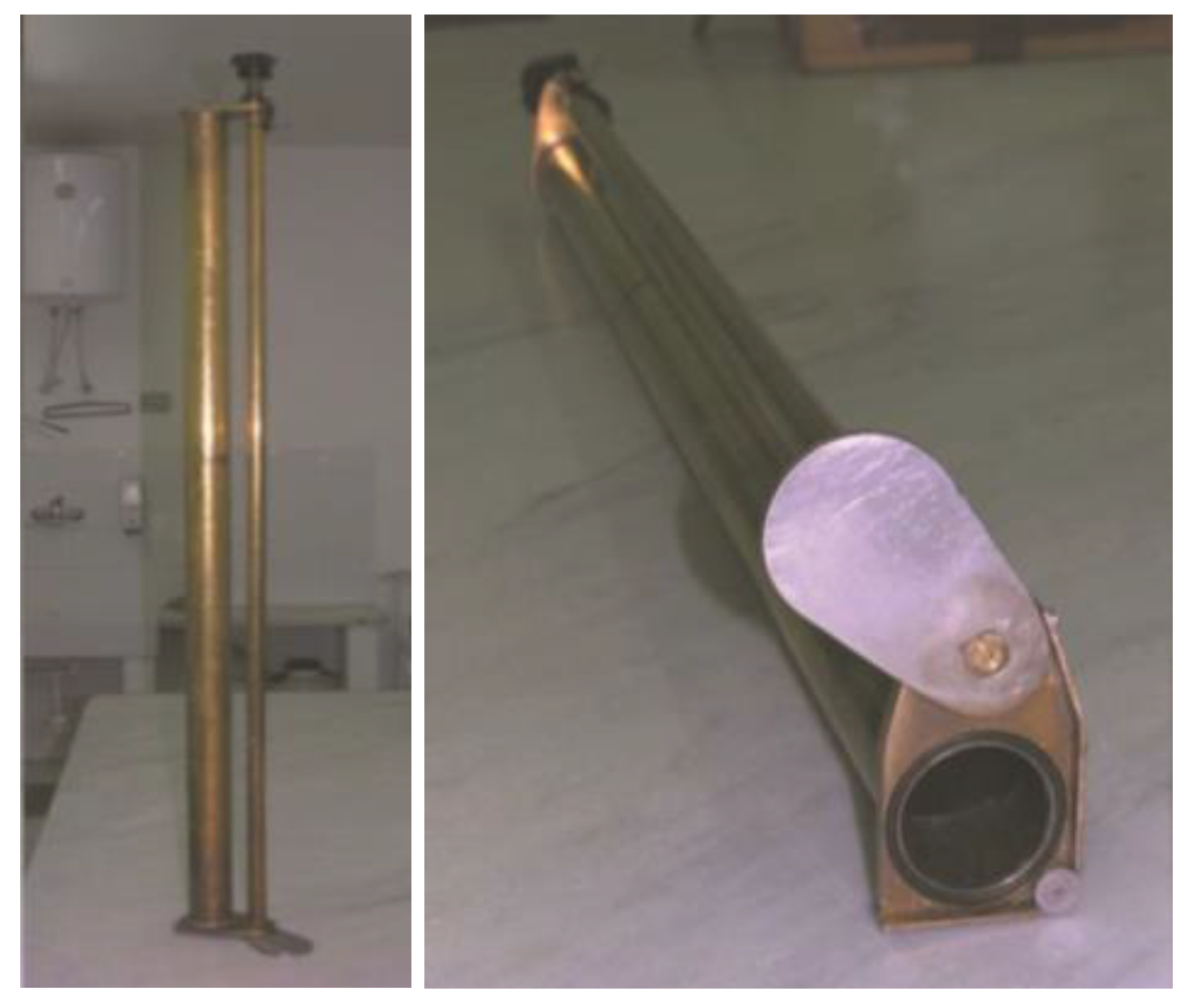
3.1. Measurement Methods

The total weight of the solid particles in the suspension collected into each tank is calculated as mean concentration by volume. The latter is easily determined by the water level reading. In order to measure mean concentration, two different procedures were applied over the monitoring period. By using the former procedure, after mixing the suspension for a given time, the sediment is sampled from 10 taps deployed along the middle vertical of the tank wall to determine the sediment concentration profile and, by integration, the mean concentration (Figure 2b). The samples are oven-dried at 105 °C for 48 h, and both the sediment weight and the associated water volume are determined. The measured mean sediment concentration differs from the actual concentration Ce as the sampling procedure determines an incomplete mixing condition, and sedimentation phenomena occur over the sampling time [19,20,25]. The measured mean concentration is then converted into the actual concentration using the calibration curve of the storage system [6,19]. According to the calibration curve, the actual concentration is equal to four-fold the measured mean concentration. When considering the high number of equipped plots in the experimental area, the above procedure was highly time-consuming for both the field sampling phase and the oven-drying one in the laboratory. Therefore, since September 2013, a quick sampling procedure using an efficient sampler has been applied [24]. The sampler is a brass cylinder with a height of 120 cm and an inner diameter of 4.75 cm. It is equipped with a closing valve ‘guillotine’ fitted with a sealing gasket (Figure 3). The valve is controlled from above using a knob joined to a drive pin. The sampler allows the extraction of a whole column, i.e., bounded by the free surface and the tank bottom of the suspension. The sampling procedure adopted in the field is based on the analysis of laboratory measurements performed by Carollo et al. [24]. Specifically, this analysis allowed us to establish that the mean value of the measured concentration in different verticals can be considered equal to the actual concentration, i.e., this sampling procedure does not need a calibration curve of the storage system, and that five samples are sufficient to obtain a relatively low margin of error. The margin of error decreases sharply as the actual concentration increases.

3.2. Experimental Results

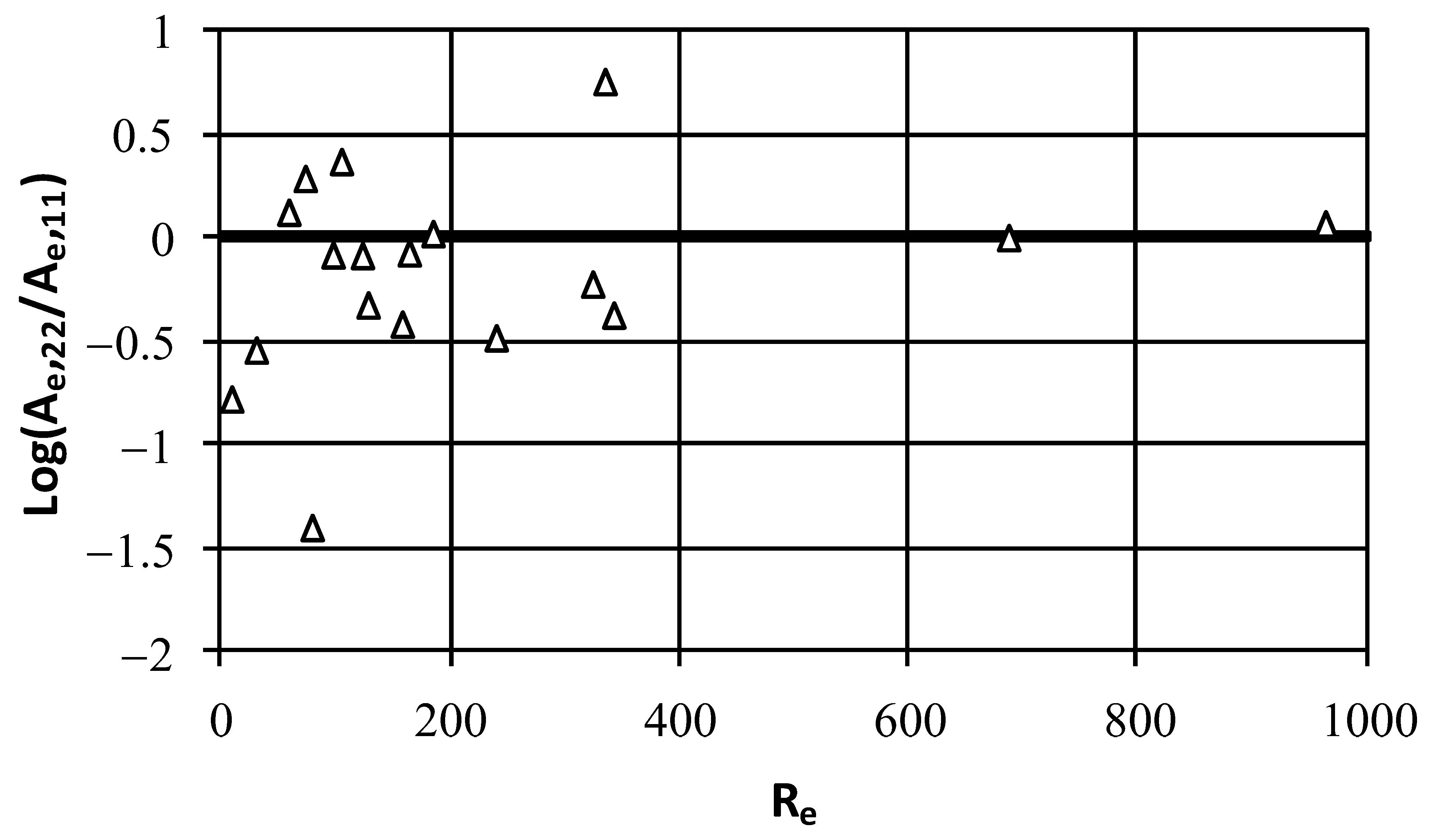
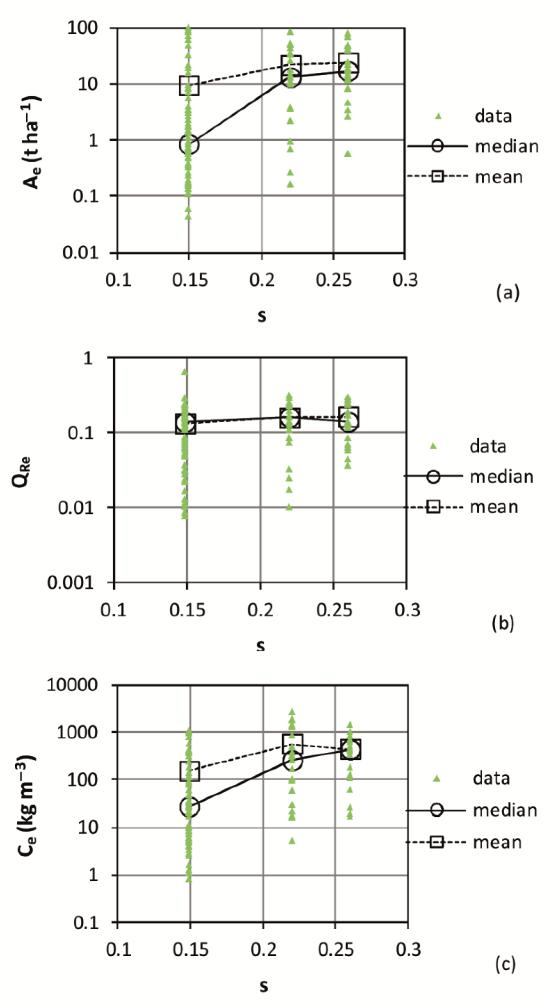
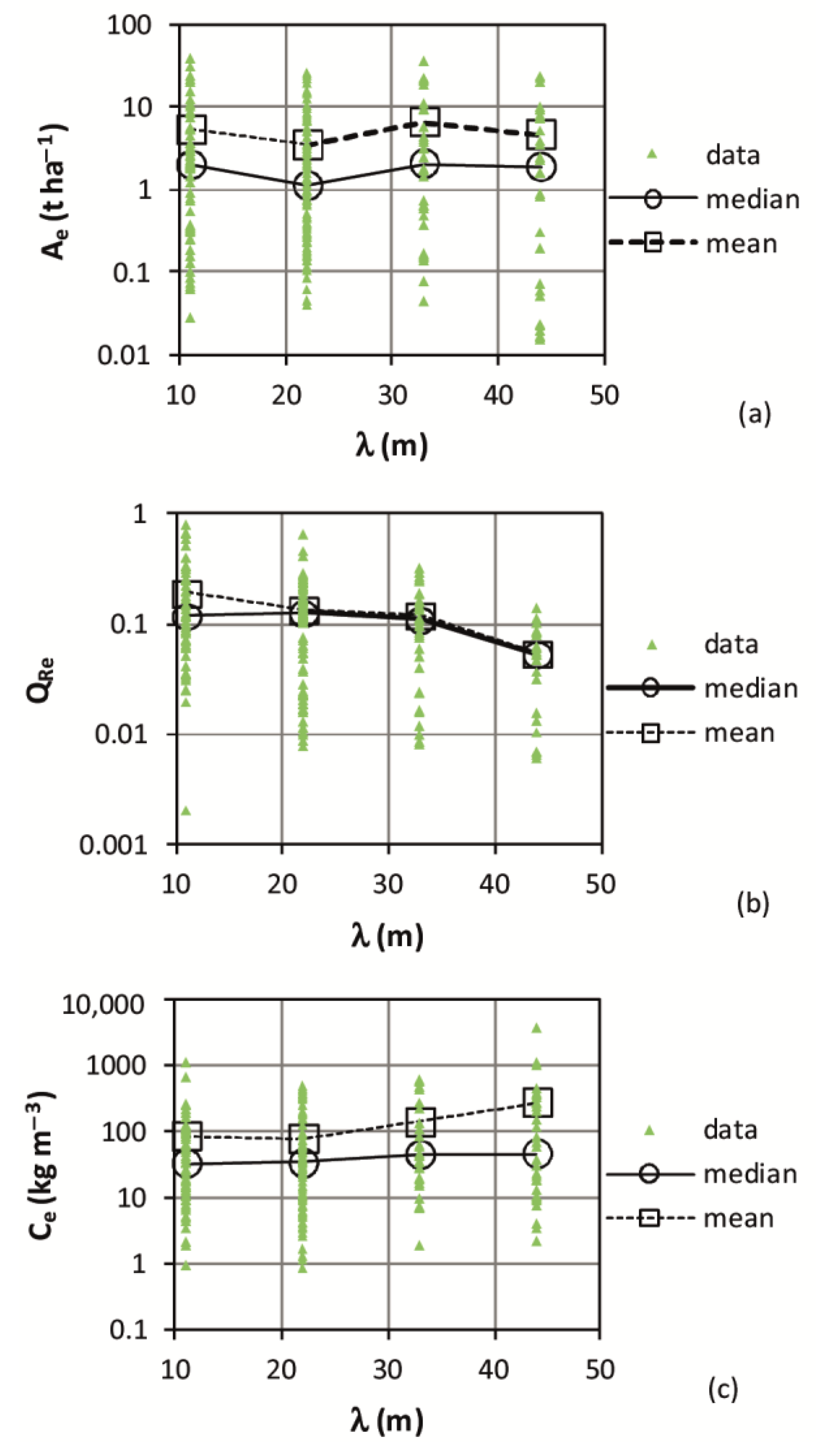
3.2.1. Effects of Plot Size and Steepness

Plot size is expected to affect soil loss due to spatial variability in infiltration, the potential for sediment to be trapped by roughness components and other sinks, and changes in erosion rates and processes with increasing amounts of runoff [26,27].
Bagarello and Ferro [28] selected 19 events monitored during the period November 1999–October 2008 to assess the effects of plot length, λ, on event soil loss per unit plot area Ae, runoff volume per unit plot area Ve, and sediment concentration Ce. The most frequent results were that soil loss did not vary significantly with λ, runoff decreased as plot length increased, and sediment concentration generally did not vary significantly with λ. Therefore, shortening the plot length was not an effective practice to control event soil loss for the Sparacia area. The analysis of the measurements of the interrill and rill erosion components available for two events supported the idea that shortening λ produces a moderate decrease in rill erosion rates but also an appreciable increase in interrill erosion rates and that shortening λ becomes effective when rill erosion is dominant (λ ≥ 33–44 m) (Figure 4). Bagarello et al. [29] investigated the plot width and length effects on Ae, Ve, and Ce by using data collected on plots differing in width (2–8 m) and length (11–22 m). A reduced data set in terms of plot length was considered to compare the results with those available at the Masse station [25]. Plot width did not have a statistically significant effect on long-term mean values of runoff, soil loss, and sediment concentration, while the plot width effects at the event temporal scale varied from negligible to significant for low erosivity events and tended to vanish for highly erosive events. Plot length did not have a statistically significant effect on mean runoff, soil loss, and sediment concentration. Moreover, in this case, for low erosivity events, the plot length effect varied from negligible to significant, while it greatly decreased for highly erosive events (Figure 5). Similar results were obtained for Masse station, characterized by soil with a prevailing silt fraction. Accordingly, both long-term and severe storm-related data collected on narrow and short plots are expected to be representative of wider and longer plots. For low erosivity events, local soil conditions at the beginning of the rainfall and more relevant measurement errors likely produced varying plot width and length effects. For highly erosive events, the importance of local soil conditions and the measurement error is reduced, and the effects of plot size on the measured variables tended to vanish. The analysis of the measurements of the interrill and rill erosion components available for an additional event to those analyzed by Bagarello and Ferro [28] highlighted that shortening λ increased total erosion since the rill erosion rate decreased, but more deposition of sediment coming from the rill channels occurred within the 22 m long plots relative to the 11 m long plots. In other words, rill interruption within the plot, which prevents the sediment from contributing to total soil loss measured at the plot outlet, was more frequent on the longer plot.
Bagarello et al. [30] established plot length and steepness effects on Ae, Ce, and the event runoff coefficient QRe, i.e., Ve per unit rainfall depth, using measurements collected until February 2012. The database was developed by considering, for a given event, the individual plots yielding a simultaneous measurement of both Ae and Ve. A total of 317 data were collected for the plots with λ = 11, 22, 33, and 44 m and s = 14.9% were considered for testing plot length effects. The selected events were those with the simultaneous functioning of at least a plot for each length to obtain reasonably homogeneous and comparable data. The 278 data collected for the 22 m long plots with s = 14.9, 22, and 26% were considered for testing plot steepness effects. The selected events were characterized by the simultaneous functioning of at least a plot for each steepness value. The mean and median values of the erosive and hydrological variables, which were expressive of the long-term average responses, confirmed that, generally, Ae did not vary appreciably with λ because the decrease in runoff coefficient was offset by an increase in sediment concentration (Figure 6). Therefore, how the physical erosion process occurred at the sampled site was not consistent with the assumption made in the USLE/RUSLE that soil loss per unit area increases with plot length. The authors verified that the short duration of individual rain showers, which determines a flow discontinuity along the hillslope [31], can favor the occurrence of more noticeable sediment deposition on longer plots, determining practically constant Ae values on plots differing in length. The moderately increasing relationship of Ce against λ was attributed to the advanced sediment transport efficiency on the longest plots, where concentrated flow, which notoriously has a higher capacity to transport sediment as compared to the overland flow, is expected to be more pronounced.
Moreover, for the event of October 2011, for λ varying from 22 to 44 m Ae decreased because of increasing rill erosion rates and increasing deposition phenomena in the interrill areas. These behaviors agree with the preceding ones obtained by Bagarello and Ferro [28] and Bagarello et al. [29] with reduced databases.
Slope steepness s had a positive effect on Ae because of a runoff coefficient QRe that did not vary appreciably with s and a sediment concentration Ce increasing with s (Figure 7). The detected steepness effects were well reproduced by the relationships used in the USLE/RUSLE models to predict the slope steepness factor. The availability of the rill and interrill erosion rates for three sampled events on 14.9 and 22% sloped plots (λ = 22 m) did not reveal clear slope effects on the rill, interrill, and total soil loss rates.
Bagarello and Ferro [32] checked plot-scale effects on hydrological and erosion variables using a larger dataset as compared with that considered by Bagarello et al. [30]. Similar information on the scale effects was obtained with four different scenarios combining dependent variables, i.e., individual values of Ae, Ve, and Ce for each plot or the mean of their replicated values, and scale indicators, i.e., plot length, λ, or plot area, A. Following Chen et al. [33], Bagarello and Ferro [32] checked scale effects using common regression analysis techniques to fit a power relationship of Ae, Ve, and Ce against λ or the plot area A to the data. The power exponent, b1, which is the scaling exponent, represented a measure of the scale effect on the considered variable. Statistically significant relationships were detected for a minor part of the sampled events, regardless of the considered variables and scenarios (19–43%).
Therefore, the lack of any scaling effect was the most common result while, when scale effects were detected, runoff always decreased, sediment concentration generally increased, and soil loss per unit area most frequently decreased in longer or larger plots. For the scenario with the largest number of scale effects, i.e., individual values of the considered variable against plot length, further analysis confirmed that lack of scale effects was the prevailing result and, when scale effects were detected, runoff decreased, sediment concentration generally increased, and soil loss per unit area generally decreased with λ. For the latter two variables, scale effects were highly dependent on the event (high variability of b1 with the event), while they showed a reduced variability with the event for runoff (reduced variability of b1 with the event). Rainfall characteristics were not able to discriminate between significant and nonsignificant scale effects. For events with a significant correlation, for the Ve − λ relationship, the exponent b1 became less negative with an increase in both rainfall amount and erosivity. In other words, scale effects for runoff were less evident when heavy rainfall occurred. The rainfall characteristics were not able to describe b1 variations for Ce and Ae.
An alternative approach was finally developed for testing scale effects with reference to the whole historical sequences of events, regardless of the single events. A statistical check was performed to establish if the probability distribution of Ae for λ = 11 m was able to reproduce the empirical frequency distribution of Ae for λ = 44 m and vice versa. The discrepancy between the probability and frequency distributions indicated the occurrence of scale effects.

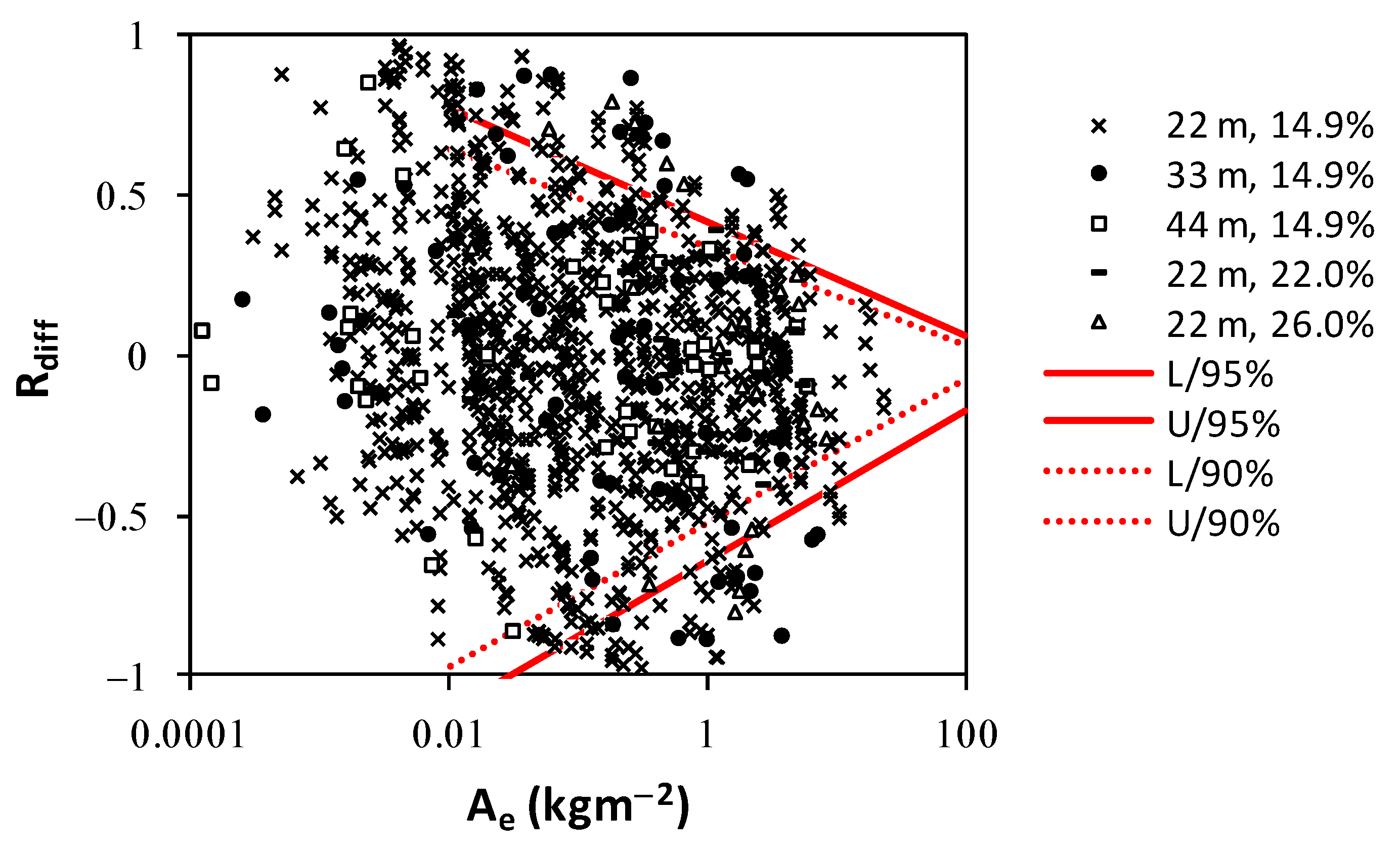
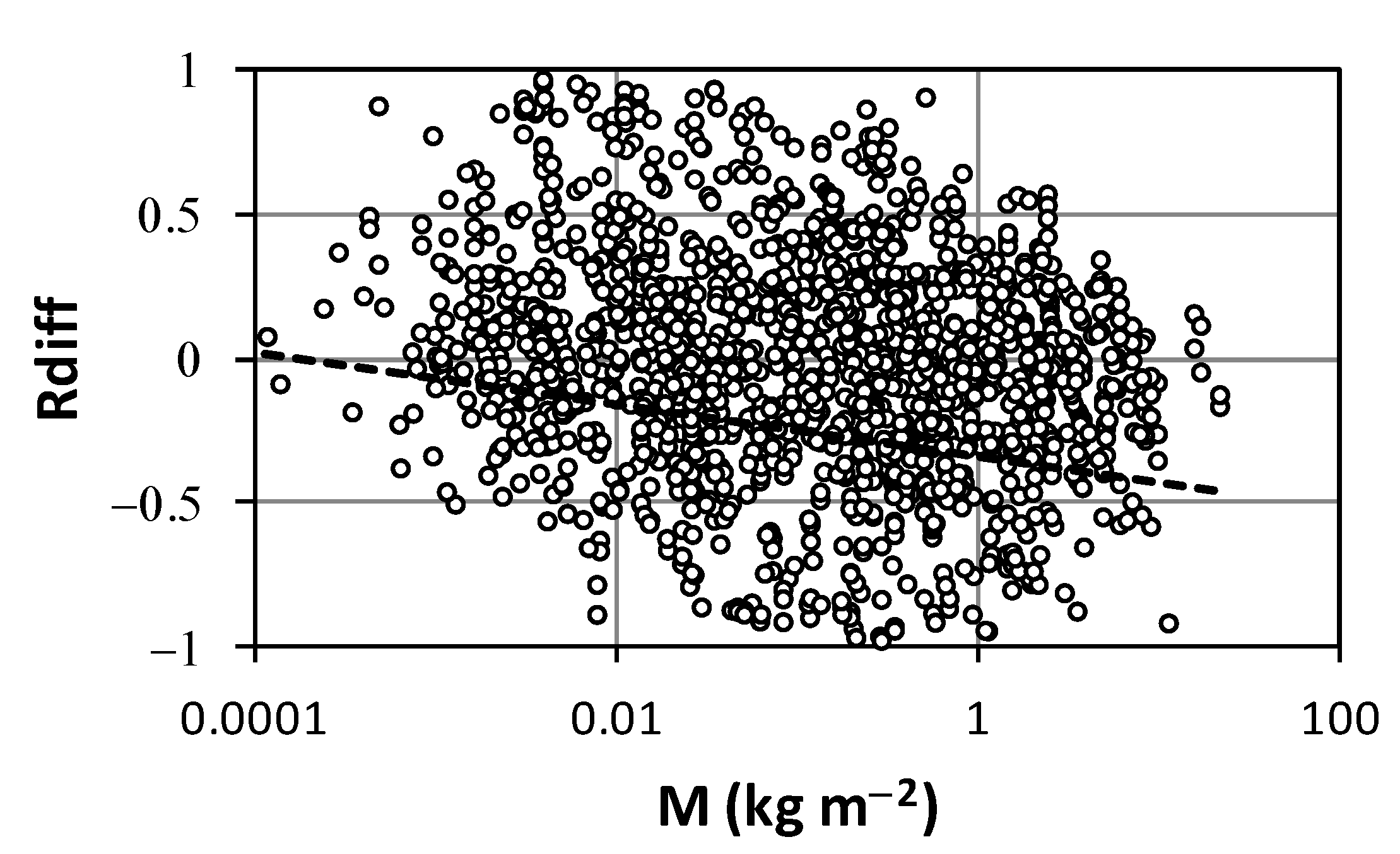
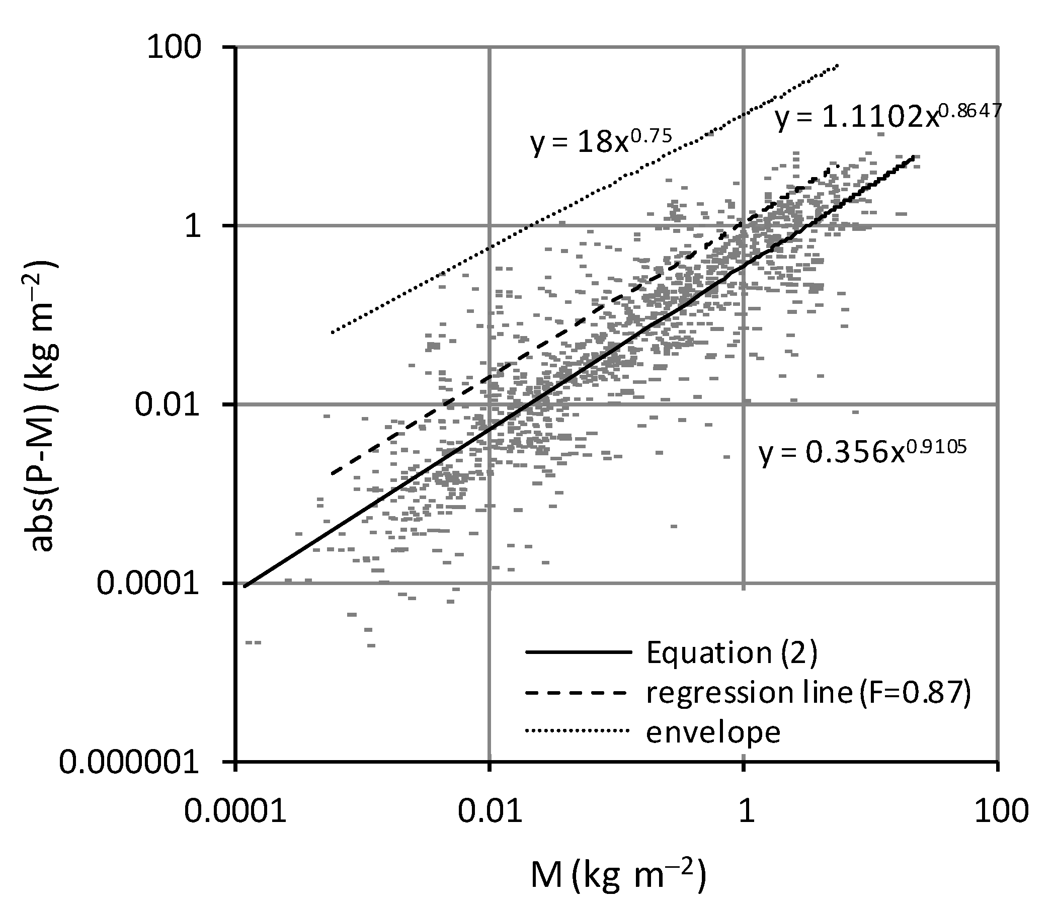
3.2.2. Measurement Variability and Physical Model Concept

Soil loss measurements are affected by a measurement variability due to the applied measurement technique [19] and a natural variability [34] that produces an unexplained variance of runoff and soil loss measurements in identical plots subjected to the same rainfall events. As a consequence of the natural variability, the single or few plot measurements are not coincident with the expected mean value for a particular treatment.
The information derived by Bagarello and Ferro [35] from measurements collected in the period 2000–2001 on 8 m × 22 m plots suggested that the coefficient of variation CV of Ae decreases as the mean measured value increases. Then, Bagarello et al. [36], by using 5 years of data from plots differing in length, highlighted that the variability of both runoff and soil loss measurements decreases as the mean value increases. This trend was detected above a threshold mean value of 3 mm for Ve and 0.1 t ha−1 for Ae, while a relatively low variability was generally detected for mean values lower than the threshold one. The analysis of the events that occurred until October 2008 [28] on 8 m × 22 m plots, jointly with the literature plot measurements, clarified that the relative variability of soil loss, runoff volume, and sediment concentration decreased as the mean measured value increased all over the experimental range. This analysis also indicated that runoff and sediment concentration were generally less variable than soil loss measurements and allowed to obtain, for each variable, a decreasing CV vs. mean relationship useful to estimate the optimum number of replicated plots for erosion studies [34,37], i.e., allowing to determine a representative value of the variable for given experimental conditions.
The natural variability of plot soil erosion measurements raises the problem of their usability to test the applicability of erosion prediction models, which is performed by comparing the measurements to the model estimations for a given temporal interval. Indeed, the difference between the measured and predicted value is due to both model error and unexplained variance of the measurements. Nearing [38] suggested a method for evaluating the performances of the model by accounting for the natural variability of plot data. According to the author, the best possible model to predict the erosion from an area of land is a physical model of the area that has similar soil type, land use, size, shape, slope (i.e., a replicated plot), and erosive inputs. Nearing [39], using a large USA soil loss database, suggested that the model prediction has to be considered acceptable if the departure from the measured value lies within the population of differences between pairs of measured values.
Bagarello and Ferro [40] tested the physical model concept by Nearing [39] using erosion data collected on the 33 m and 44 m long plots and the 22 m long plots established on 14.9%, 22%, and 26% slopes from November 1999 to April 2011. The relative difference, Rdiff, was calculated as follows [39]:
R d i f f = P M P + M
where P is the predicted value from the physical model and M is the measured value. In order to define the physical model, differences in width between the plot and its replicate were neglected. The highest measured values showed fewer relative differences between replicates (Figure 8), in accordance with the results obtained by Nearing [39]. The Rdiff data falling within the empirically calculated 95% occurrence interval (Equation (3) in [39]) were equal to 88% of the total. When considering the relatively low discrepancy between these percentages, the investigation supported the applicability of the analysis by Nearing [39] for model evaluations. Bagarello et al. [41] used bare plot soil loss data (November 1999–May 2012) from Sparacia and Masse experimental stations. A total of 819 Ae values were available, varying from 0.00012 to 21.7 kg m−2. The Italian (P, M) database was compiled by considering four plot lengths (λ = 11, 22, 33, and 44 m), four slope steepness values (s = 14.9, 16.0, 22.0, and 26.0%), and defining a physical model as a plot with the same length and width to the sampled one.
Indeed, the preliminary linear regression analysis between the M and P values suggested that the physical model has to be defined in terms of perfect planimetric equivalence. The percentage of Rdiff values falling within the 95% occurrence interval (Equation (3) in [39]) was equal to 88.9%, which was in line with the previous result by Bagarello and Ferro [40]. However, Rdiff values decreasing with an increase in M, which is the premise of the analysis by Nearing [39], were only detected for M > 1 kg m−2, and the corresponding Rdiff values falling within the 95% occurrence interval were equal to only 85.1% of the total (Figure 9). Accordingly, a new applicative criterion of the physical model concept was developed and expressed by the following relationship between the absolute difference between the physical model prediction and measurement (Figure 10):
| P M | = 0.356 M 0.91
where R2 = 0.72. For a given soil loss value (M), Equation (2) predicts the mean absolute difference associated with the sampling of a replicated plot. A model prediction is acceptable if the absolute difference with the measured soil loss is lower than or equal to the value calculated by Equation (2).
The general objective of the investigation by Bagarello et al. [42] was to compare the two applicative criteria of the physical model concept by Nearing [39] (original criterion) and Bagarello et al. [41] (new criterion) through three soil erosion empirical models and plot soil loss data from Sparacia. The criterion by Bagarello et al. [41], which was expressed in terms of Rdiff to be directly comparable with that of Nearing [39], was analytically demonstrated to be characterized by a greater selectivity. Indeed, the fraction of the acceptable model predictions relative to the total varied from 29% for the former to 54% for the latter.
A less restrictive new criterion was developed by carrying out a frequency analysis of all the data used to obtain Equation (2). In particular, the data were divided into half log-cycle intervals, and within each division, the value associated with a frequency higher than 0.5, which practically yields Equation (2), was determined. The power regression equation between the values associated with a frequency F of 0.87 and M values (Figure 10) featured a similar selectivity level as that of the original criterion. Both the original and new criteria accept predictions characterized by relative maximum errors that decrease as M increases. For example, Equation (2) accepts predictions with a maximum error decreasing from 80% to 27% as M increases from the minimum (0.00012 kg m−2) to the maximum (21.7 kg m−2) value. Based on all available data, the models’ accuracy ranking depended on the evaluation criterion, while for the highest soil losses, both criteria gave the same accuracy ranking. In order to increase the significance of the comparison between the two criteria, they should be calibrated by merging the American and Italian databases.

3.2.3. Statistical Analysis of Soil Loss Measurements

Field investigations (e.g., [43]) have clearly shown that rare and severe events control total soil erosion over a long period. Consequently, soil conservation strategies should be developed considering soil loss of a given return period rather than long-term average erosion.
Bagarello et al. [44] developed a frequency analysis of relatively long-term (2000–2008) soil loss data collected in a high number of simultaneously operating plots and microplots of different lengths (λ = 0.25, 0.4, 11, 22, 33, and 44 m) and slope of 14.9%. This analysis allowed establishing both the theoretical distribution reproducing the frequency distribution and the soil loss of a given return period. Each event’s soil loss value, Ae, measured on a plot of given length λ, was normalized using the mean soil loss, μ(Ae), calculated for that event and all the plots with the same length. Normalization allowed assuming that the probability distribution P(x) of the variable x = Ae/μ(Ae) is unique. For both the microplots and plots, the frequency distributions of x were perfectly overlapping, and thus P(x) was independent of both the scale length λ and the temporal scale, which were completely represented by the mean value, μ(Ae).
For a given plot length, the values (334 data) of the annual maximum event soil loss were then extracted from the complete dataset (1403 data). As the x frequency distributions for both the complete dataset and the annual maxima were overlapping, the parameters of the probability distribution of the annual maximum soil loss and the quantiles of a given return period were estimated using all available data. The empirical frequency distribution of x was described by a two-component distribution (Figure 11), with the two components discriminated by a return period of 25 years. The soil loss of a given return period was estimated by multiplying the mean soil loss by a frequency factor determined by fitting Gumbel’s distribution to the two components of the frequency distribution.
The subsequent study by Bagarello et al. [45] was conducted using soil loss measurements from individual plots in the period from November 1999 to January 2009. First, this study confirmed the results by Bagarello et al. [44] that the distribution of the normalized soil loss does not vary with λ, and the parameters of the probability distribution of the annual maximum soil loss and the quantiles of a given return period can be estimated using all available data. Then, the authors deduced that, according to the USLE scheme applied at the event temporal scale, the soil loss of a given return period is obtained by amplifying the mean soil loss for a sequence of events by a frequency factor estimated with the frequency distribution of the rainfall erosivity index. The reliability of this deduction was verified by the available measurements of rainfall erosivity index and event soil loss for each considered plot length. Assuming that this result is also valid at the annual temporal scale, an estimating criterion of the annual soil loss of a given return period was developed. By this criterion, the probability distribution of the yearly rainfall erosivity factor, which is available for the Sicilian region, can be used to design soil conservation practices.

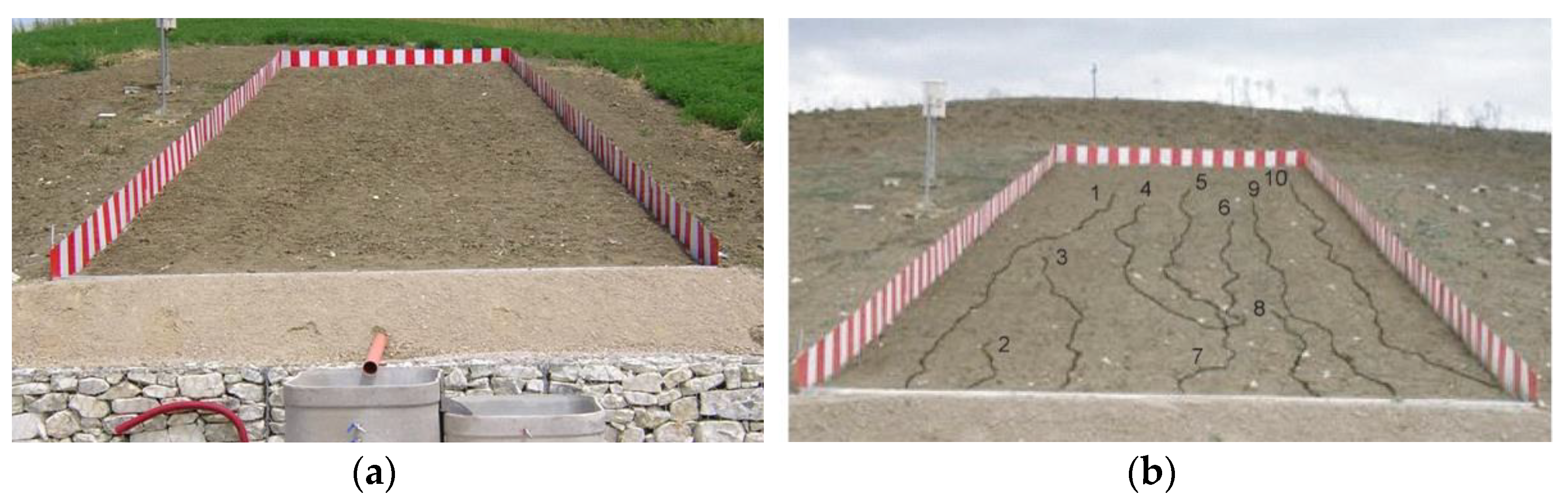
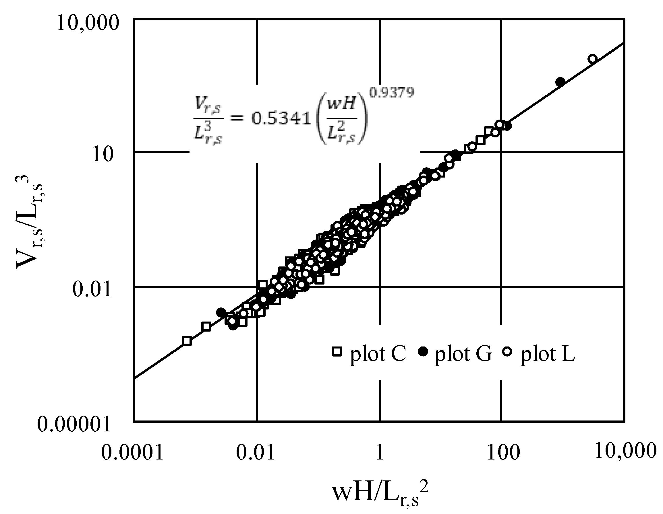
4. Measurement of Rill Erosion at Sparacia

4.1. Measurement Methods

Rill erosion measurements were firstly performed by the traditional direct method and, more recently, applying an indirect technique (image-based) [46,47,48,49,50,51,52,53,54,55,56,57,58,59,60]. In the former case [1,61,62,63,64,65], the rill channels were visually identified in the field and divided into segments bounded by two measurement cross-sections with a varying distance interval depending on the variability of rill depth, width, and appearance of tributaries along the rill length (Figure 12). On average, this distance interval was equal to 2 m. In order to measure the rill segment features, i.e., mean width w, maximum scour depth H, and cross-section area σ, a rillmeter [61] was used. The rill segment length Lr,s was measured by a metric ruler. Specifically, the values of w, H, and σ were set equal to the mean of the values measured at the bounding sections, and the rill segment volume Vr,s was equal to σ Lr,s. The plan-altimetric survey of the rill network was carried out using a total station, and the segment slope was determined along the rill thalweg. The widely used direct method is very simple, low-cost [66], and invasive as the operators tend to modify the surface of the rilled area. In addition, it was time-consuming due to the high number of experimental plots established at the Sparacia station.
Advancements in automatic 3D-photo reconstruction techniques induced us to apply the Structure from Motion (SfM) technique (image-based) to measure rill erosion using low-altitude aerial [62,67] and terrestrial acquisition platforms [67]. Image-based modeling creates a three-dimensional Digital Terrain Model (3D-DTM) using a set of oblique photographs taken from the same rilled surface [68] with uncalibrated and non-metric cameras, coupled with photogrammetric software packages, such as Photoscan professional (Agisoft). Camera model parameters and scene geometry are simultaneously solved [69], using redundant information coming from oblique photographs. The generated 3D point cloud has to be scaled and georeferenced using some ground control points (GCPs) located within the monitored rilled area. Di Stefano et al. [67] deployed six GCPs on the plot perimeter (Figure 13) and collected their (x, y, z) coordinates with a total station. From the 3D point cloud, a 2.5D surface (i.e., Digital Elevation Model, DEM) and the orthophoto were also generated. Unlike DEM, which represents the surface of the rilled area from a vertical perspective, the 3D-DTM can also represent cross-section areas with undercut walls [68] where different z-elevations can be associated with the same couple of plane coordinates x–y. In this case, the DEM underestimates the area of the cross-section and, therefore, the eroded rill volume [70]. However, the DEM is often used for hydrological analyses, and it can be easily managed as it is a raster model.
In order to extract channel networks from DEM, Carollo et al. [62] applied both a manual method, which consisted of tracing rills from the visual interpretation of orthophotos, and an automatic procedure based on the theory of drop analysis by Broscoe [71]. In the last case, drainage paths were identified by following the maximum slope direction and by all of the cells of the DEM with a value of drainage area greater than an established threshold. The value of this threshold was obtained by the drop analysis. By using the hierarchical approach of Horton and Strahler, Broscoe [71] defined drop as the height difference between the two points defining a channel from the source/confluence to the confluence with another stream. According to Broscoe [71], the threshold value of drainage area is that for which the drop mean values, calculated for each stream order, are almost equal.
Di Stefano et al. [67] applied a method based on the combination of a drainage algorithm and the convergence index CI, which is defined by the following relationship:
C I = ( 1 n 1 i = 1 n 1 θ i ) 90
where n is the number of kernel cells, and for each external cell i, θi (°) is the angle between the aspect of the cell and the direction of the vector joining the center of the cell and the center of the kernel [72]. The convergence index ranges from −90° to 90°. Positive values relate to divergent areas, negative values relate to convergent areas, and null values represent areas without curvature as planar slopes. In order to determine cells that should correspond to the rill channel, an objective threshold, beyond which the CI values could be considered significantly different from a plane landform, was set equal to two times the standard deviation, std, of CI [73]. When considering that only negative CI values relate to convergent areas, significant flow convergence cells were characterized by CI ≤ −2 std. At the end of this step, the disconnected convergent areas were identified and considered as rill features. In order to achieve the connection, the flow accumulation algorithm was weighted with the threshold convergence grid following Thommeret et al. [72]. Finally, a grid representing the rill thalweg was obtained. Rills detected by Di Stefano et al. [67] were automatically separated into contributing rills, which were connected to the network reaching the plot outlet and contributed to total soil loss measured at the plot outlet and non-contributing rills, which were interrupted within the plot (Figure 13). Each contributing rill was divided into segments, each of them bounded by two 0.25 m long transects perpendicular to the rill thalweg and spaced 0.3 m apart, and Vr,s was calculated as 0.3 σ. The use of the SfM technique allowed for obtaining accurate rill erosion measurements with rapid and not invasive field surveys but time-consuming image post-processing.
For both direct and indirect measurement methods, the total rill volume V was calculated by adding the volumes Vr,s, and converted into the weight of eroded soil by the soil bulk density. The latter was experimentally determined on different dates by collecting soil samples uniformly distributed on the erosion plots. Soil samples were taken by cylindric samplers [74], with a diameter of 8 cm and a height of 5 cm, and oven-dried at 105 °C for 48 h.

4.2. Experimental Results

In the monitoring period from September 2004 to February 2006, Bruno et al. [61] carried out measurements on rills formed on a 22% sloping plot in five erosion events. The authors verified the applicability of a power relationship between rill length L and rill volume V; thereby, rill length can be employed to estimate the severity of the rilling process. By applying the Π-theorem of the dimensional analysis and the incomplete self-similarity hypothesis [75,76], they also proposed a power dimensionless relationship among the rill morphological variables (length Lr,s, width w, depth H, and volume Vr,s). Di Stefano and Ferro [63] pointed out that the scale parameter of the L-V relationship varies with channel type (rills, Ephemeral Gullies (EGs), and gullies) while the exponent is constant. Moreover, the authors verified that the above power dimensionless relationship describes a morphological similarity between the channels of rills, EGs, and gullies.
The analysis of the rill cross-sections detected by Bruno et al. [61] along the channel highlighted changes from the narrow and deep upstream sections to enlarged downstream sections conserving the depth. In the terminal reach, the cross-section area diminished because of a decreasing flow transport capacity due to rill slope reduction.
Di Stefano et al. [1] extended the available database, including measurements collected in the year 2008 on all the plots established in the experimental area. The availability of measurements carried out on different slopes (14.9, 22, and 26%) allowed detection of the influence of the plot slope on rill width and depth. In particular, for a given flow discharge and increasing slope values, the rills deepened and narrowed. Di Stefano et al. [1] validated the L-V (Figure 14) and the power dimensionless (Figure 15) relationships previously calibrated by Di Stefano and Ferro [63].
The reliability of these equations was further confirmed by Di Stefano et al. [64] using rill measurements performed in the event of October 2011. In this case, the indirect survey of the rill network was also conducted, for the first time at Sparacia, by an Unmanned Aerial Vehicle (UAV). Rills tracks were derived from the visual interpretation of orthophotos. For a single plot of 8 m × 44 m, Di Stefano et al. [64] compared the L-V pairs and the two groups of the power dimensionless relationship detected both with the direct and indirect measurement method and pointed out the consistency of the results obtained with the two methods.
Di Stefano et al. [64] proposed a simplified method to estimate the rill erodibility based on the simplifying assumptions concerning temporal variability of the bottom shear stress and wetted perimeter and neglecting the effect of sediment load on flow detachment. The application of the method requires only the knowledge of the geometric characteristics of the rills at the end of the erosion event and the duration of the event and gives a first approximation of the rill erodibility. Rill erodibility values were relatively low compared to those reported on a global dataset regarding field plot experiments on agricultural soils [77]. This result agrees with the relatively low value of the USLE erodibility factor for the Sparacia soil [78]. The rill erodibility variation between plots was negligible, and the plot erodibility was not stationary. The method was also validated by using the Water Erosion Prediction Project (WEPP) database for the condition ‘rainfall plus flow addition at the head of each rill’, which showed that a reliable value of rill erodibility could be obtained for 71 rills of 27 USA experimental sites [65].
For an 8 m × 44 m plot and the event of October 2011, Carollo et al. [62] compared the rill cross-sections obtained by both the direct method (rillmeter) and DEM jointly with the manual method to identify flow paths. By assuming the rillmeter measurements as a reference, the analysis showed that the indirect method provided lower values of depth and higher values of surface width, resulting in a substantial invariance of the cross-section area. The automatic extraction of the rill network by the drop analysis detected a higher number of rills and longer compared to those detected by the manual method, highlighting the difficulty of identifying rills in the downstream end of the plot from visual observation of the orthophoto. The measurements obtained with the automatic extraction of the rills for three 22, 33, and 44 m long plots confirmed the applicability of the L-V (Figure 16) and the power dimensionless (Figure 17) relationships, which were calibrated by Di Stefano and Ferro [63] by measurements performed by rillmeter and a metric ruler. In other words, the calibration coefficients of these equations were independent of the survey method.
Di Stefano et al. [67] applied the SfM technique with a terrestrial (TS) and a UAV survey of rills formed on two 6 m × 22 m plots with the steepness of 22% and 26% during a rainfall event in October 2016. In order to increase the density of the UAV point cloud, for the 22% sloping plot, a further point cloud was built, merging all aerial photos and 40 terrestrial photos (UAV + TS survey). Rill network extraction was performed by the CI method, and the drainage density, i.e., the total length of rills per unit plot area, and the drainage frequency, i.e., the number of rill segments per unit plot area, were determined. For each of the four combinations plot—rill type (i.e., contributing and not contributing)—the highest values of drainage density (ranging from 0.74 to 1.45 m m−2) and drainage frequency (ranging from 0.25 to 0.85 m−2) were measured by TS, denoting its better capability of detecting rills, which was consistent with the highest density of the 3D point cloud. In order to investigate the plot slope, s, effect on the morphometric parameters, their mean values obtained by different surveys were used. The ratio between the contributing rill length and the total length was significantly higher for s = 26% (64%) than for s = 22% (45%). Moreover, for contributing rills, the available measurements and the literature data [79] indicated that the drainage density increases with plot steepness, whereas an opposite trend occurs for non-contributing rills (Figure 18). Both the results showed an increase in the connectivity degree and thus the efficiency of the sediment transport system, with plot steepness.
A further analysis aimed to compare the amount of sediment stored in the tank with the rill component due to contributing rills. When considering the former as a reference value (DM, Figure 19), soil loss measurement error by the 3D model was equal to 6% (TS) and −6% (UAV) for the 26% sloping plot and equal to 13% (TS), −8% (UAV), and 10% (UAV + TS) for the 22% sloping plot (Figure 19). In any case, these errors were within the margin of error of the reference value for a probability level of 5% [23], which was equal to ±10.4% for the 26% sloping plot (Ce = 390 g L−1), and equal to ±13.1% for the 22% sloping plot (Ce = 282 g L−1). Finally, this analysis confirmed the reliability of the SfM measurement technique.

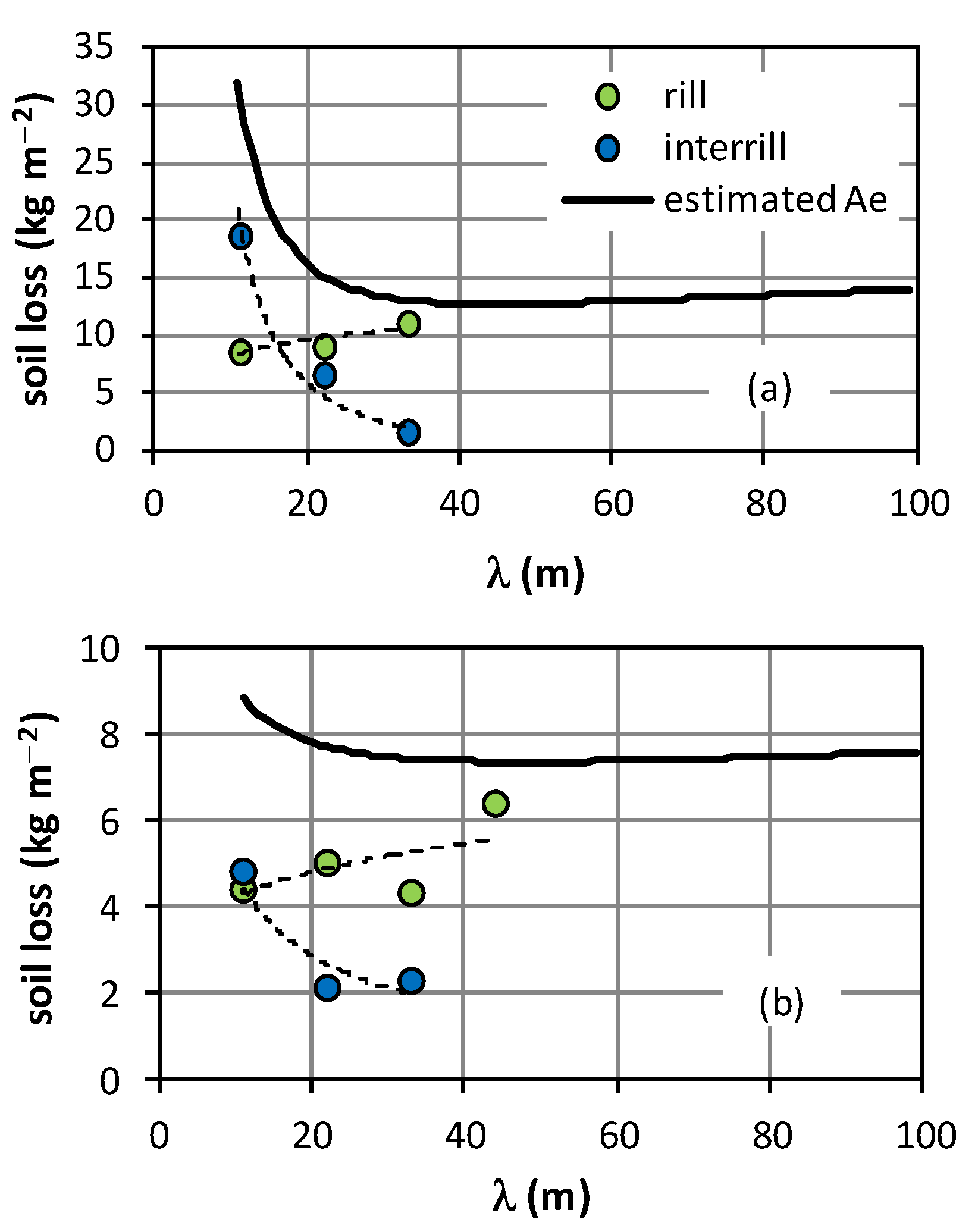
5. Comparing Interrill and Rill Erosion

A first attempt to determine the relative importance of interrill and rill erosion on total soil loss was carried out by Bagarello and Ferro [35] by using the data collected on the 8 m × 22 m plots and square microplots of different lengths (0.2 and 0.4 m) and areas. The study examined three events in the period of April–December 2000, for which soil loss data were available for the three plot types. In the microplots, only interrill erosion likely occurred while rills developed in the USLE-plots. For a given event, a mean value of soil loss per unit area was determined by averaging the data collected in all operating plots of a given surface area. For each event, soil loss decreased in the passage from the smaller to the larger microplots. The straight line passing through the two data points representative of the microplots was extrapolated to the USLE-plot area to estimate the interrill soil erosion (Figure 20a). In this case, the rill component was obtained as the difference between total (rill + interrill) soil loss and the interrill component determined by extrapolation of the straight line. In all events, interrill soil erosion was a minor or negligible part of total soil erosion (0.1–7.1%). Methodological improvements, including the use of other microplot sizes (1 × 1, 1 × 2, 1 m × 5 m), were applied by Di Stefano et al. [64]. Their analysis was carried out using all soil loss measurements by microplots and USLE-plots established on the 14.9% slope simultaneously working for a given event in the period 2000–2013. The data points corresponding to 1 m × 5 m microplots aligned with those of other microplots in some events, whereas they were over the interrill line in other events (Figure 20b,c). Therefore, a plot length equal to 5 m was sufficient for the occurrence of rill erosion processes, at least in some events. The data points representative of the measurements carried out on USLE plots only aligned with those representatives of the microplots for four events, indicating that only interrill erosion occurred. For most events, rill erosion was dominant as it ranged from 70% to 99.9% of total soil erosion measured in the different plots. Moreover, the rill erosion rate was not dependent on the rainfall erosivity factor, as evaluated by the USLE approach, which varied from 42.7 MJ mm ha−1 h−1 to 686.3 MJ mm ha−1 h−1.
The investigation by Bruno et al. [61] was conducted by measuring total soil loss and the direct survey of the rill channels in a plot 6 m × 22 m with s = 22% in the period September 2004–February 2006. For the five events for which a rill network developed, rill erosion was equal, on average, to 69.5% of total soil loss, and interrill erosion ranged from 193 to 4183 g m−2. For the five events for which rills were not visually detectable, interrill erosion was assumed to be coincident with total soil loss and ranged from 10 to 96 g m−2. The comparison between the interrill erosion rates for the two cases pointed out the interaction between rill and interrill processes. Indeed, the presence of a rill network promotes the transport efficiency of the sediments coming from the interrill areas. These sediments are transported by overland flow into the rill channels where the rill flow, which is characterized by a higher velocity than the overland flow, can effectively transport them and sediment particles detached from the rill wetted perimeter.
Di Stefano et al. [1] extended the investigation by Bruno et al. [61] by using the direct surveys of the rill channels performed in all the plots but two of the experimental station in the period 2004–2008 for a total of 41 plot-event combinations. The authors detected rill erosion higher than total soil loss for almost one-half of combinations and attributed this result to the occurrence of sediment delivery processes for the not contributing rills. Indeed, they calculated rill erosion from both contributing and not contributing rills, overestimating then the rill sediment that had reached the downstream tank. The occurrence of sediment delivery processes could not be excluded even if rill erosion was less than total soil loss. However, in this case, the rill erosion rates, calculated by neglecting possible sediment delivery processes, ranged between 24% and 94% of the total soil loss, with a mean value equal to 63%. As a general result, rill erosion was confirmed to be dominant relative to interrill erosion.
For testing the reliability of the aforementioned method based on the extrapolation of the interrill line, Di Stefano et al. [64] compared the rill erosion estimated by this method and that obtained by the direct survey of the rills. This comparison was possible for a single erosion event for which rill erosion was detected by the two methods. When assuming the direct measurement as a reference, the absolute error generally varied from 11% to 36%, indicating quite satisfactory reliability of the method based on the interrill line.

6. Conclusions

Efficient management of a large experimental station for soil erosion measurement needs the use of methods and procedures that can guarantee a rapid and accurate field measurement. Currently, in the Sparacia plots, this is obtained by a quick sampling procedure using an efficient cylindrical sampler to measure total soil loss and by the Structure from Motion technique to measure the rill component.
The main results that were obtained during the extended monitoring period can be summarized by the following points:
  • The long-term average soil loss per unit area generally did not vary appreciably with the plot length because the decrease in runoff coefficient was offset by an increase in sediment concentration. Moreover, the analysis at the event scale suggested that soil loss per unit area most frequently decreased in longer plots. In any case, these results were not consistent with the assumption made in the USLE/RUSLE model. On the contrary, the long-term steepness effect was well reproduced by the predictive relationships of the USLE/RUSLE slope steepness factor;
  • The relative variability of soil loss, runoff volume, and sediment concentration decreased as the mean measured value increased, and soil loss measurements were generally more variable than runoff volume and sediment concentration. In order to account for the natural variability of the soil loss measurements in the evaluation of the predictive capability of the erosion models, a new applicative criterion of the physical model concept was developed using measurements performed at the Sparacia and Masse experimental stations;
  • In the sampled site, for a given plot length, the soil loss of a given return period can be estimated by multiplying the mean soil loss by a frequency factor. The latter is determined by fitting Gumbel’s distribution to the two components of the frequency distribution of the normalized event soil loss;
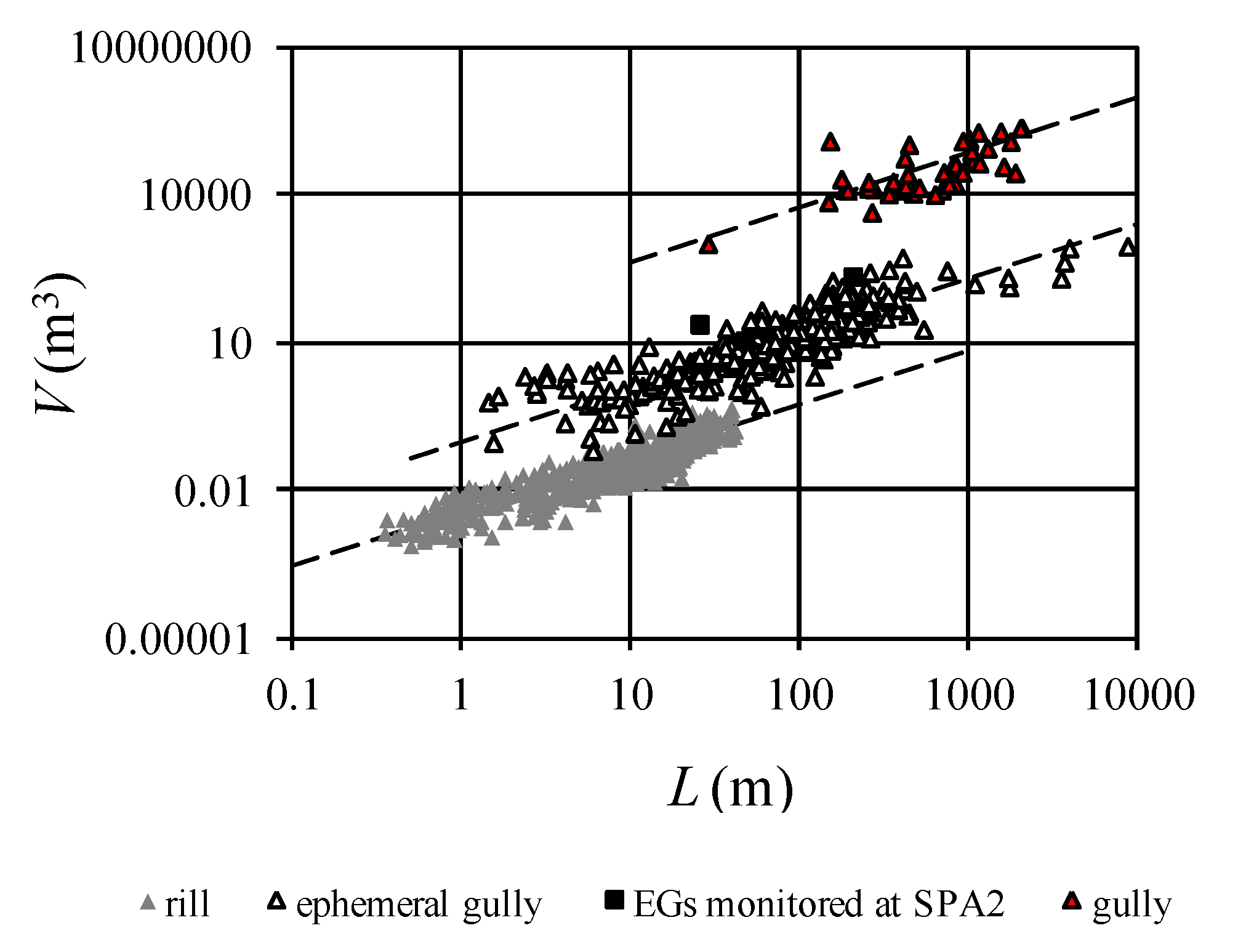
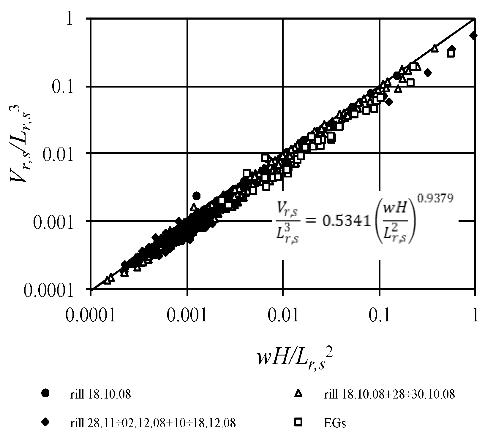
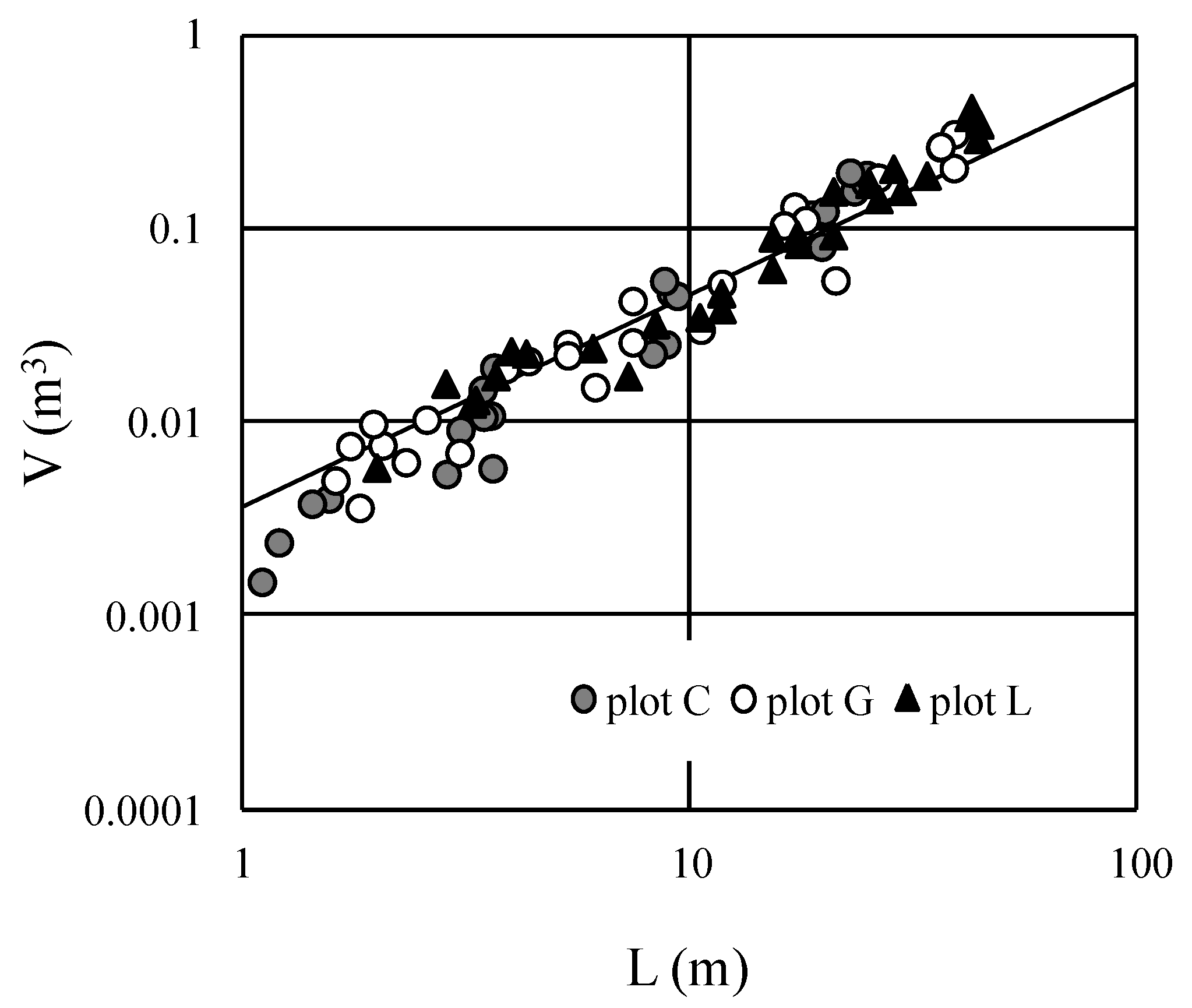
  • The measurements of the rill volumes and lengths allowed us to verify the reliability of a power relationship between the two variables. The measurements also confirmed the morphological similarity between the channels of the rills and EGs described by a power dimensionless relationship;
  • The rill erodibility of the clay soil of Sparacia was estimated by a simplified method, which was also validated by using the WEPP database. Rill erodibility varied over time, maintaining relatively low values;
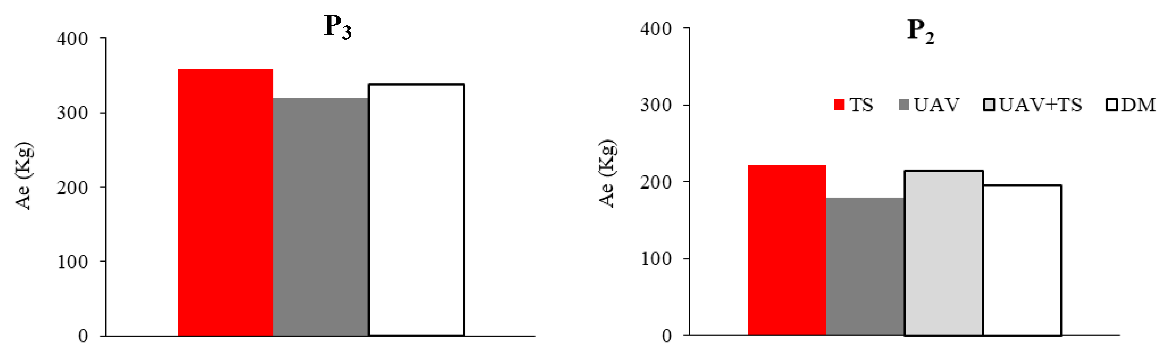
  • The reliability of the SfM technique to measure rill erosion was positively tested;
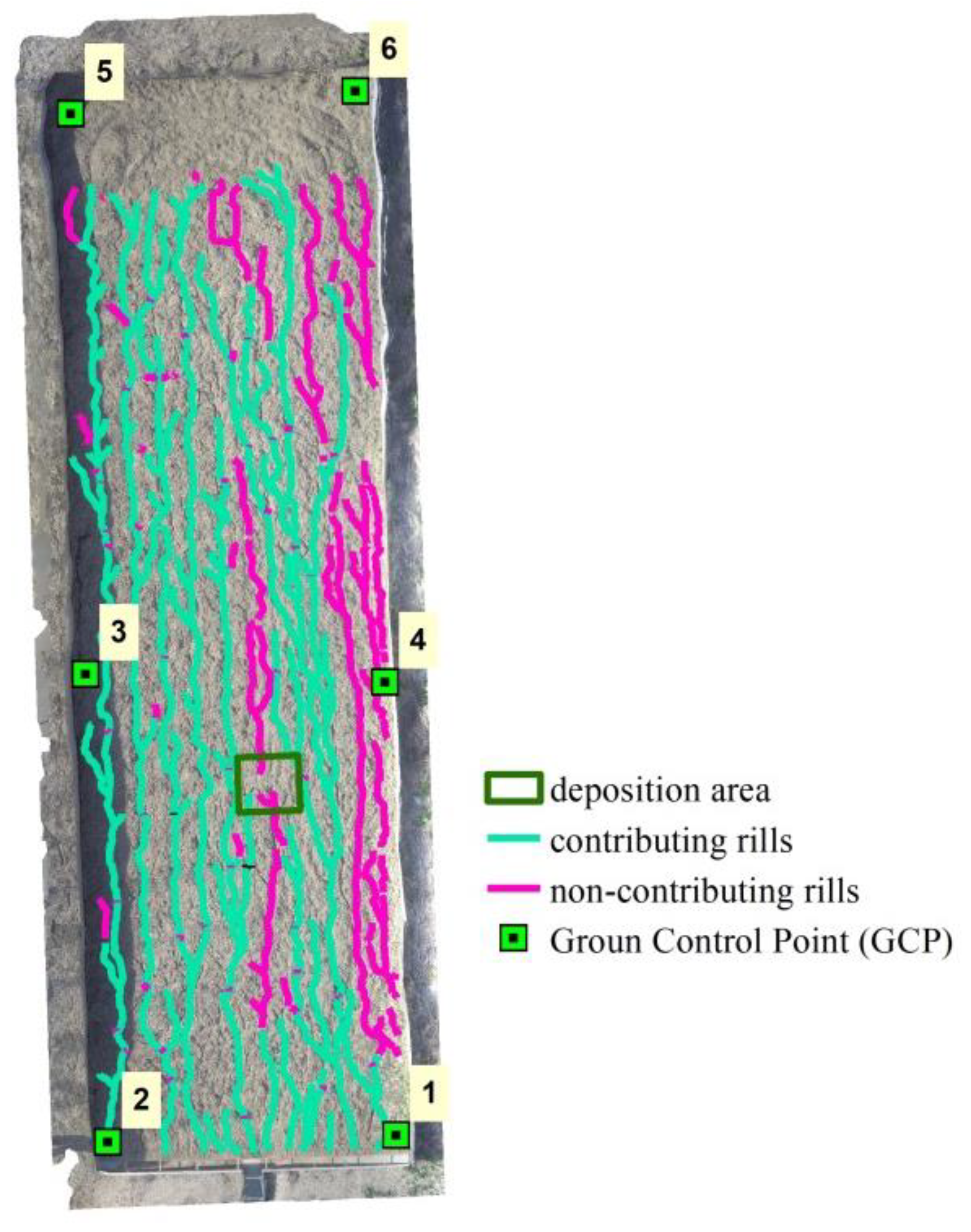
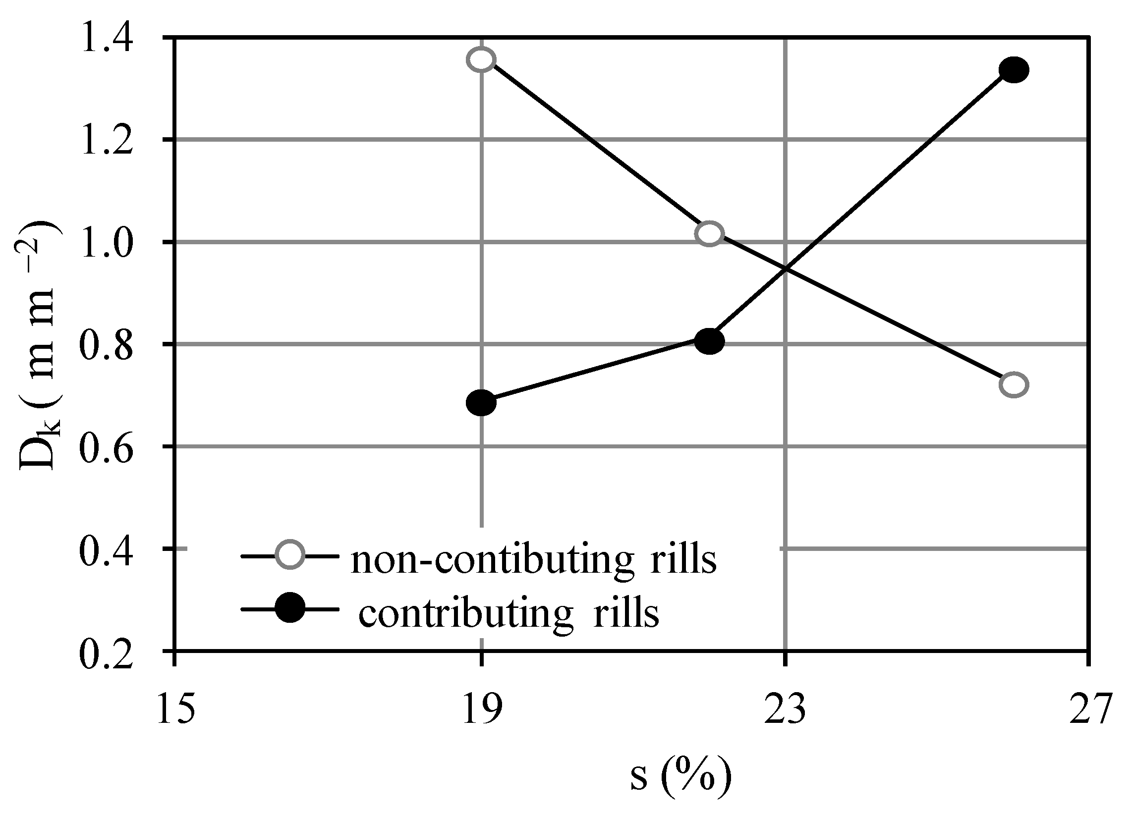
  • For the contributing rills, the drainage density increased, indicating a more efficient sediment transport system as plot steepness increased;
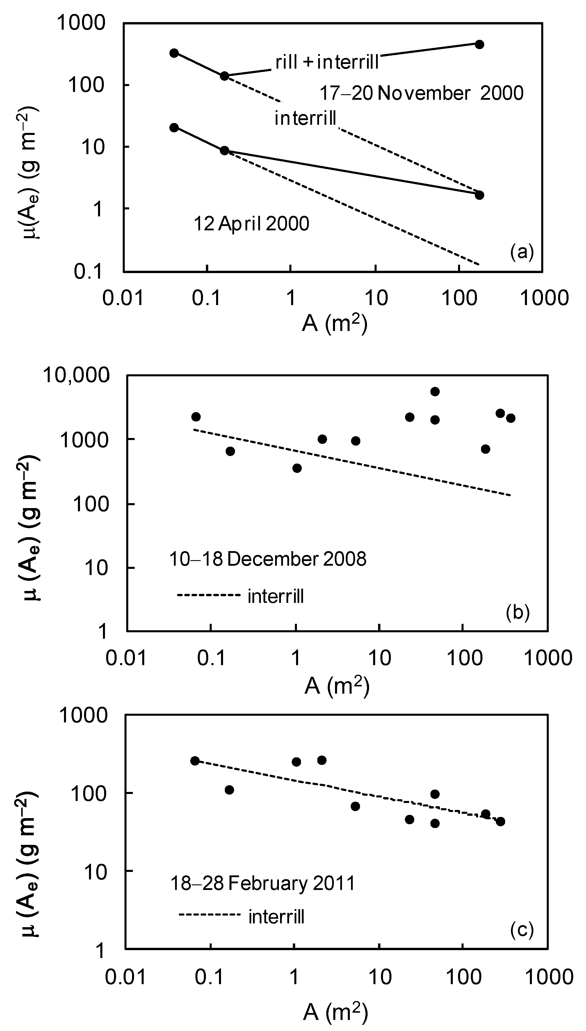
  • As a general result, rill erosion was dominant relative to interrill erosion.
Further research could be developed to increase the reliability of the new applicative criterion of the physical model concept, e.g., by using data from the American database, while further soil loss measurements in the Sparacia station could be used to update the frequency analysis.
Moreover, the dynamics of a rill network during a rainfall season could be investigated. Rill channels are usually obliterated after each erosion event to re-establish plot standard conditions, while for this purpose, rills would not be deleted. Multi-temporal surveys, using the SfM technique, could allow for assessing the hydrological and erosive responses of plots with pre-existing rills when rainfall event occurs.
Finally, future research activities could benefit from the upgrade of the experimental site with an optical disdrometer to measure both the size and falling velocity of the raindrops. These measurements allow for determining the rainfall kinetic energy. Considering that, for given plot characteristics (soil, steepness, size), variations in soil loss exclusively depend on variations in rainfall characteristics, that is, according to the USLE-type models, on variations in rainfall erosivity, the soil loss measurement is proportional to the measurement of rainfall erosivity. Therefore, the comparison between soil loss measurements with intensity and kinetic energy of the rainfall can permit verifying if the rainfall erosivity is adequately represented by the current erosion models or if they need to be improved.

Author Contributions

Conceptualization, V.P. (Vincenzo Pampalone), F.G.C., A.N., V.P. (Vincenzo Palmeri), C.D.S., V.B. and V.F.; methodology, V.P. (Vincenzo Pampalone), F.G.C., A.N., V.P. (Vincenzo Palmeri), C.D.S., V.B. and V.F.; formal analysis, V.P. (Vincenzo Pampalone), F.G.C., A.N., V.P. (Vincenzo Palmeri), C.D.S., V.B. and V.F.; writing—review and editing, V.P. (Vincenzo Pampalone), F.G.C., A.N., V.P. (Vincenzo Palmeri), C.D.S., V.B. and V.F. All authors have read and agreed to the published version of the manuscript.

Funding

This research received no external funding.

Institutional Review Board Statement

Not applicable.

Informed Consent Statement

Not applicable.

Data Availability Statement

No new data were created or analyzed in this study. Data sharing is not applicable to this article.

Conflicts of Interest

The authors declare no conflict of interest.

References

  1. Di Stefano, C.; Ferro, V.; Pampalone, V.; Sanzone, F. Field investigation of rill and ephemeral gully erosion in the Sparacia experimental area, South Italy. Catena 2013, 101, 226–234. [Google Scholar] [CrossRef]
  2. Bagarello, V.; Ferro, V.; Pampalone, V. A comprehensive check of USLE-based soil loss prediction models at the Sparacia (south Italy) site. In Innovative Biosystems Engineering for Sustainable Agriculture, Forestry and Food Production, MID-TERM AIIA 2019; Coppola, A., Di Renzo, G., Altieri, G., D’Antonio, P., Eds.; Lecture Notes in Civil Engineering; Springer: Cham, Switzerland, 2020; Volume 67, pp. 3–11. [Google Scholar]
  3. Bagarello, V.; Ferro, V.; Pampalone, V. A comprehensive analysis of USLE-based models at the Sparacia experimental area. Hydrol. Process. 2020, 34, 1545–1557. [Google Scholar] [CrossRef]
  4. Bagarello, V.; Ferro, V.; Flanagan, D.C. Predicting plot soil loss by empirical and process-oriented approaches. A review. J. Agric. Eng. 2018, 49, 1–18. [Google Scholar] [CrossRef]
  5. Bagarello, V.; Di Stefano, C.; Ferro, V.; Pampalone, V. Comparing theoretically supported rainfall-runoff erosivity factors at the Sparacia (South Italy) experimental site. Hydrol. Process. 2018, 32, 507–515. [Google Scholar] [CrossRef]
  6. Bagarello, V.; Di Piazza, G.V.; Ferro, V. Manual sampling and tank size effects on the calibration curve of plot sediment storage tanks. Trans. ASAE 2004, 47, 1105–1112. [Google Scholar] [CrossRef]
  7. Chaplot, V.; Le Bissonnais, Y. Field measurement of interrill erosion under different slopes and plot sizes. Earth Surf. Process. Landf. 2000, 25, 145–153. [Google Scholar] [CrossRef]
  8. Brakensiek, D.L.; Osborn, H.B.; Rawls, W.J. Field Manual for Research in Agricultural Hydrology. USDA Agricultural Handbook; USDA: Washington, DC, USA, 1979.
  9. Boix-Fayos, C.; Martínez-Mena, M.; Calvo-Cases, A.; Arnau-Rosalén, E.; Albaladejo, J.; Castillo, V. Causes and underlying processes of measurement variability in field erosion plots in Mediterranean conditions. Earth Surf. Process. Landf. 2007, 32, 85–101. [Google Scholar] [CrossRef]
  10. Cerdà, A.; Brazier, R.; Nearing, M.; de Vente, J. Scales and Erosion. Catena 2013, 102, 1–2. [Google Scholar] [CrossRef]
  11. Parsons, A.J.; Brazier, R.E.; Wainwright, J.; Powell, D.M. Scale relationships in hillslope runoff and erosion. Earth Surf. Process. Landf. 2006, 31, 1384–1393. [Google Scholar] [CrossRef]
  12. Boix-Fayos, C.; Martínez-Mena, M.; Arnau-Rosalén, E.; Calvo-Cases, A.; Castillo, V.; Albaladejo, J. Measuring soil erosion by field plots: Understanding the sources of variation. Earth Sci. Rev. 2006, 78, 267–285. [Google Scholar] [CrossRef]
  13. Sadeghi, S.H.R.; Bashari Seghaleh, M.; Rangavar, A.S. Plot sizes dependency of runoff and sediment yield estimates from a small watershed. Catena 2013, 102, 55–61. [Google Scholar] [CrossRef]
  14. Bagarello, V.; Ferro, V. Measuring soil loss and subsequent nutrient and organic matter loss on farmland. In Oxford Research Encyclopedias, Environmental Science; Oxford University Press: Oxford, UK, 2017; p. 47. [Google Scholar]
  15. Carter, C.E.; Parsons, D.A. Field test on the Coshocton-type wheel runoff sampler. Trans. ASAE 1967, 10, 133–135. [Google Scholar]
  16. Bazzoffi, P. Fagna-type hydrological unit for runoff measurement and sampling in experimental plot trials. Soil Technol. 1993, 6, 251–259. [Google Scholar] [CrossRef]
  17. Bonilla, C.A.; Kroll, D.G.; Norman, J.M.; Yoder, D.C.; Molling, C.C.; Miller, P.S.; Panuska, J.C.; Topel, J.B.; Wakeman, P.L.; Karthikeyan, K.G. Instrumentation for Measuring Runoff, Sediment and Chemical Losses. J. Environ. Qual. 2006, 35, 216–223. [Google Scholar] [CrossRef] [PubMed]
  18. Pierson, F.B., Jr.; Van Vactor, S.S.; Blacbum, W.H.; Wood, J.C. Incorporating small scale spatial variability into predictions of hydrologic response on Sagebrush Rangelands. In Variability of Rangeland Water Erosion Processes; Soil Science Society of America Special Publication: Madison, WI, USA, 1994; Volume 38. [Google Scholar]
  19. Bagarello, V.; Ferro, V. Calibrating storage tanks for soil erosion measurement from plots. Earth Surf. Process. Landf. 1998, 23, 1151–1170. [Google Scholar] [CrossRef]
  20. Lang, R.D. Accuracy of two sampling methods used to estimate sediment concentrations in runoff from soil-loss plots. Earth Surf. Process. Landf. 1992, 17, 841–844. [Google Scholar] [CrossRef]
  21. Zobisch, M.A.; Klingspor, P.; Oduor, A.R. The accuracy of manual runoff and sediment sampling from erosion plots. J. Soil Water Conserv. 1996, 51, 231–233. [Google Scholar]
  22. Ciesiolka, C.A.A.; Yu, B.; Rose, C.W.; Ghadiri, H.; Lang, D.; Rosewell, C. Improvement in soil loss estimation in USLE type experiments. J. Soil Water Conserv. 2006, 61, 223–229. [Google Scholar]
  23. Nikkami, D. Investigating sampling accuracy to estimate sediment concentrations in erosion plot tanks. Turk. J. Agric. For. 2012, 36, 583–590. [Google Scholar]
  24. Carollo, F.G.; Di Stefano, C.; Ferro, V.; Pampalone, V.; Sanzone, F. Testing a new sampler for measuring plot soil loss. Earth Surf. Process. Landf. 2016, 41, 867–874. [Google Scholar] [CrossRef]
  25. Todisco, F.; Vergni, L.; Mannocchi, F.; Bomba, C. Calibration of the soil loss measurement method at the Masse experimental station. Catena 2012, 91, 4–9. [Google Scholar] [CrossRef]
  26. Wischmeier, W.H.; Smith, D.D. Predicting Rainfall Erosion Losses. A Guide to Conservation Planning. USDA Agriculture Handbook No. 537; USDA: Hyattsville, MD, USA, 1978.
  27. Cerdà, A.; Bodì, M.B.; Burguet, M.; Segura, M.; Jovani, J. The plot size effect on soil erosion on rainfed agriculture land under different land uses in eastern Spain. In Geophysical Research Abstract; EGU2009-185-1; EGU General Assembly 2009; Copernicus Publications: Göttingen, Germany, 2009; Volume 11. [Google Scholar]
  28. Bagarello, V.; Ferro, V. Analysis of soil loss data from plots of differing length for the Sparacia experimental area, Sicily, Italy. Biosyst. Eng. 2010, 105, 411–422. [Google Scholar] [CrossRef]
  29. Bagarello, V.; Ferro, V.; Giordano, G.; Mannocchi, F.; Pampalone, V.; Todisco, F.; Vergni, L. Effect of plot size on measured soil loss for two italian experimental sites. Biosyst. Eng. 2011, 108, 18–27. [Google Scholar] [CrossRef]
  30. Bagarello, V.; Ferro, V.; Pampalone, V. Testing assumptions and procedures to empirically predict bare plot soil loss in a Mediterranean environment. Hydrol. Process. 2015, 29, 2414–2424. [Google Scholar] [CrossRef]
  31. Yair, A.; Raz-Yassif, N. Hydrological processes in a small arid catchment: Scale effects of rainfall and slope length. Geomorphology 2004, 61, 155–169. [Google Scholar] [CrossRef]
  32. Bagarello, V.; Ferro, V. Scale effects on plot runoff and soil erosion in a mediterranean environment. Vadose Zone J. 2017, 16, 1–14. [Google Scholar] [CrossRef]
  33. Chen, L.; Sela, S.; Svoray, T.; Assouline, S. Scale dependence of Hortonian rainfall–runoff processes in a semiarid environment. Water Resour. Res. 2016, 52, 5149–5166. [Google Scholar] [CrossRef]
  34. Nearing, M.A.; Govers, G.; Norton, L.D. Variability in soil erosion data from replicated plots. Soil Sci. Soc. Am. J. 1999, 63, 1829–1835. [Google Scholar] [CrossRef]
  35. Bagarello, V.; Ferro, V. Plot-scale measurement of soil erosion at the experimental area of Sparacia (southern Italy). Hydrol. Process. 2004, 18, 141–157. [Google Scholar] [CrossRef]
  36. Bagarello, V.; Di Piazza, G.V.; Ferro, V.; Giordano, G. Predicting unit plot soil loss in Sicily, South Italy. Hydrol. Process. 2008, 22, 586–595. [Google Scholar] [CrossRef]
  37. Warrick, A.W. Appendix 1: Spatial variability. In Environmental Soil Physics; Hillel, D., Ed.; Academic Press: San Diego, CA, USA, 1998; pp. 655–675. [Google Scholar]
  38. Nearing, M.A. Why soil erosion models over-predict small soil losses and underpredict large soil losses. Catena 1998, 32, 15–22. [Google Scholar] [CrossRef]
  39. Nearing, M.A. Evaluating soil erosion models using measured plot data: Accounting for variability on the data. Earth Surf. Process. Landf. 2000, 25, 1035–1043. [Google Scholar] [CrossRef]
  40. Bagarello, V.; Ferro, V. Testing the “physical model concept” by soil loss data measured in Sicily. Catena 2012, 95, 1–5. [Google Scholar] [CrossRef]
  41. Bagarello, V.; Ferro, V.; Giordano, G.; Mannocchi, F.; Pampalone, V.; Todisco, F. A modified applicative criterion of the physical model concept for evaluating plot soil erosion predictions. Catena 2015, 126, 53–58. [Google Scholar] [CrossRef]
  42. Bagarello, V.; Ferro, V.; Pampalone, V. Comparing two applicative criteria of the soil erosion physical model concept. Vadose Zone J. 2017, 16, 1–10. [Google Scholar] [CrossRef]
  43. Larson, W.E.; Lindstrom, M.J.; Schumacher, T.E. The role of severe storms in soil erosion: A problem needing consideration. J. Soil Water Conserv. 1997, 52, 90–95. [Google Scholar]
  44. Bagarello, V.; Di Stefano, C.; Ferro, V.; Pampalone, V. Statistical distribution of soil loss and sediment yield at Sparacia experimental area, Sicily. Catena 2010, 82, 45–52. [Google Scholar] [CrossRef]
  45. Bagarello, V.; Di Stefano, C.; Ferro, V.; Pampalone, V. Using plot soil loss distribution for soil conservation design. Catena 2011, 86, 172–177. [Google Scholar] [CrossRef]
  46. Di Stefano, C.; Ferro, V.; Palmeri, V.; Pampalone, V. Flow resistance equation for rills. Hydrol. Process. 2017, 31, 2793–2801. [Google Scholar] [CrossRef]
  47. Di Stefano, C.; Ferro, V.; Palmeri, V.; Pampalone, V. Flow resistance in step-pool rills. Vadose Zone J. 2017, 16, 1–10. [Google Scholar] [CrossRef]
  48. Di Stefano, C.; Ferro, V.; Palmeri, V.; Pampalone, V. Testing slope effect on flow resistance equation for mobile bed rills. Hydrol. Process. 2018, 32, 664–671. [Google Scholar] [CrossRef]
  49. Palmeri, V.; Pampalone, V.; Di Stefano, C.; Nicosia, A.; Ferro, V. Experiments for testing soil texture effects on flow resistance in mobile bed rills. Catena 2018, 171, 176–184. [Google Scholar] [CrossRef]
  50. Nicosia, A.; Di Stefano, C.; Pampalone, V.; Palmeri, V.; Ferro, V.; Nearing, M.A. Testing a new rill flow resistance approach using the Water Erosion Prediction Project experimental database. Hydrol. Process. 2019, 33, 616–626. [Google Scholar] [CrossRef]
  51. Di Stefano, C.; Nicosia, A.; Pampalone, V.; Palmeri, V.; Ferro, V. Rill flow resistance law under equilibrium bed-load transport conditions. Hydrol. Process. 2019, 33, 1317–1323. [Google Scholar] [CrossRef]
  52. Di Stefano, C.; Nicosia, A.; Palmeri, V.; Pampalone, V.; Ferro, V. Comparing flow resistance law for fixed and mobile bed rills. Hydrol. Process. 2019, 33, 3330–3348. [Google Scholar] [CrossRef]
  53. Carollo, F.G.; Di Stefano, C.; Nicosia, A.; Palmeri, V.; Pampalone, V.; Ferro, V. Flow resistance in mobile bed rills shaped in soils with different texture. Eur. J. Soil Sci. 2021, 72, 2062–2075. [Google Scholar] [CrossRef]
  54. Di Stefano, C.; Nicosia, A.; Palmeri, V.; Pampalone, V.; Ferro, V. Estimating flow resistance in steep slope rills. Hydrol. Process. 2021, 35, e14296. [Google Scholar] [CrossRef]
  55. Palmeri, V.; Di Stefano, C.; Ferro, V. A Maximizing Hydraulic Radius (MHR) method for defining cross-section limits in rills and ephemeral gullies. Catena 2021, 303, 105347. [Google Scholar] [CrossRef]
  56. Pampalone, V.; Di Stefano, C.; Nicosia, A.; Palmeri, V.; Ferro, V. Analysis of rill step–pool morphology and its comparison with stream case. Earth Surf. Process. Landf. 2021, 46, 775–790. [Google Scholar] [CrossRef]
  57. Nicosia, A.; Guida, G.; Di Stefano, C.; Pampalone, V.; Ferro, V. Slope threshold for overland flow resistance on sandy soils. Eur. J. Soil Sci. 2022, 73, e13182. [Google Scholar] [CrossRef]
  58. Di Stefano, C.; Nicosia, A.; Palmeri, V.; Pampalone, V.; Ferro, V. Rill flow resistance law under sediment transport. J. Soils Sediments 2022, 22, 334–347. [Google Scholar] [CrossRef]
  59. Nicosia, A.; Palmeri, V.; Pampalone, V.; Di Stefano, C.; Ferro, V. Slope threshold in rill flow resistance. Catena 2022, 208, 105789. [Google Scholar] [CrossRef]
  60. Nicosia, A.; Di Stefano, C.; Palmeri, V.; Pampalone, V.; Ferro, V. Evaluating the effects of the rill longitudinal profile on flow resistance law. Water 2022, 14, 326. [Google Scholar] [CrossRef]
  61. Bruno, C.; Di Stefano, C.; Ferro, V. Field investigation on rilling in the experimental Sparacia area, South Italy. Earth Surf. Process. Landf. 2008, 33, 263–279. [Google Scholar] [CrossRef]
  62. Carollo, F.G.; Di Stefano, C.; Ferro, V.; Pampalone, V. Measuring rill erosion at plot scale by a drone-based technology. Hydrol. Process. 2015, 29, 3802–3811. [Google Scholar] [CrossRef]
  63. Di Stefano, C.; Ferro, V. Measurements of rill and gully erosion in Sicily. Hydrol. Process. 2011, 25, 2221–2227. [Google Scholar] [CrossRef]
  64. Di Stefano, C.; Ferro, V.; Pampalone, V. Modelling rill erosion at the Sparacia experimental area. J. Hydrol. Eng. 2015, 20, C5014001. [Google Scholar] [CrossRef]
  65. Di Stefano, C.; Ferro, V.; Pampalone, V. Measuring field rill erodibility by a simplified method. Land Degrad. Dev. 2016, 27, 239–247. [Google Scholar] [CrossRef]
  66. Casalí, J.; Loizu, J.; Campo, M.A.; De Santisteban, L.M.; Àlvarez-Mozos, J. Accuracy of methods for field assessment of rill and ephemeral gully erosion. Catena 2006, 67, 128–138. [Google Scholar] [CrossRef]
  67. Di Stefano, C.; Palmeri, V.; Pampalone, V. An automatic approach for rill network extraction to measure rill erosion by terrestrial and low-cost UAV photogrammetry. Hydrol. Process. 2019, 33, 1883–1895. [Google Scholar]
  68. Frankl, A.; Stal, C.; Abraha, A.; Nyssen, J.; Rieke-Zapp, D.; De Wulf, A.; Poesen, J. Detailed recording of gully morphology in 3D through image-based modelling. Catena 2015, 127, 92–101. [Google Scholar] [CrossRef]
  69. James, M.R.; Robson, S. Straightforward reconstruction of 3D surfaces and topography with a camera: Accuracy and geosciences applications. J. Geophys. Res. 2012, 117, 1–17. [Google Scholar] [CrossRef]
  70. Di Stefano, C.; Ferro, V.; Palmeri, V.; Pampalone, V.; Agnello, F. Testing the use of an image-based technique to measure gully erosion at Sparacia experimental area. Hydrol. Process. 2017, 31, 573–585. [Google Scholar] [CrossRef]
  71. Broscoe, A.J. Quantitative Analysis of Longitudinal Stream Profiles of Small Watersheds; Technical Report 389-042; Department of Geology, Columbia University: New York, NY, USA, 1959. [Google Scholar]
  72. Thommeret, N.; Bailly, J.S.; Puech, C. Extraction of thalweg networks from DTMs: Application to badlands. Hydrol. Earth Syst. Sci. 2010, 14, 1527–1536. [Google Scholar] [CrossRef]
  73. Pirotti, F.; Tarolli, P. Suitability of LiDAR point density and derived landform curvature maps for channel network extraction. Hydrol. Process. 2010, 24, 1187–1197. [Google Scholar] [CrossRef]
  74. Bryan, R.B.; Hawke, R.M.; Rockwell, D.L. The influence of subsurface moisture on rill system evolution. Earth Surf. Process. Landf. 1998, 23, 773–789. [Google Scholar] [CrossRef]
  75. Barenblatt, G.I. Similarity, Self-Similarity and Intermediate Asymptotics; Consultants Bureau: New York, NY, USA, 1979. [Google Scholar]
  76. Barenblatt, G.I. Dimensional Analysis; Gordon and Breach: Amsterdam, The Netherlands, 1987. [Google Scholar]
  77. Knapen, A.; Poesen, J.; Govers, G.; Gyssels, G.; Nachtergaele, J. Resistance of soils to concentrated flow erosion: A review. Earth-Sci. Rev. 2007, 80, 75–109. [Google Scholar] [CrossRef]
  78. Bagarello, V.; Di Stefano, C.; Ferro, V.; Giordano, G.; Iovino, M.; Pampalone, V. Estimating the USLE soil erodibility factor in Sicily, South Italy. Appl. Eng. Agric. 2012, 28, 199–206. [Google Scholar] [CrossRef]
  79. Gessesse, G.; Fuchs, H.; Mansberger, R.; Klik, A.; Rieke-Zapp, D.H. Assessment of erosion, deposition and rill development on irregular soil surfaces using close range digital photogrammetry. Photogramm. Rec. 2010, 25, 299–318. [Google Scholar] [CrossRef]
Figure 1. Plan and view of the experimental plots installed on the (a) 14.9% slope and (b) 22% and 26% slopes (modified from [1]).
Water 14 01881 g001
Figure 2. View of the (a) storage tanks and (b) concentration profile (modified from [6]).
Water 14 01881 g002
Figure 3. View of the sampler (modified from [24]).
Water 14 01881 g003
Figure 4. Relationship of total, Ae, rill, and interrill soil loss vs. plot length, λ, for the (a) 1 September 2005 event and (b) 28 June 2008 event (modified from [28]).
Water 14 01881 g004
Figure 5. Log of the ratio between soil losses, Ae, measured in the plots with length λ = 22 m and plots with λ = 11 m vs. the erosivity index, Re (MJ mm ha−1 h−1) (modified from [29]).
Water 14 01881 g005
Figure 6. Plot length, λ, effect on event (a) soil loss per unit area, Ae, (b) runoff coefficient, QRe, and (c) sediment concentration, Ce, for the plots with slope steepness s = 14.9% (modified from [30]).
Water 14 01881 g006
Figure 7. Plot steepness, s, effect on event (a) soil loss per unit area, Ae, (b) runoff coefficient, QRe, and (c) sediment concentration, Ce, for the 22 m long plots (modified from [30]).
Water 14 01881 g007
Figure 8. Relative differences in measurements of soil loss between replicated plots, Rdiff, vs. the measured soil loss value, M, for all plots established at the Sparacia station and 90 and 95% occurrence intervals for the data (L = lower limit; U = upper limit) calculated according to [39] (modified from [40]).
Water 14 01881 g008
Figure 9. Relative differences in the measurement of soil loss between replicated plots, Rdiff, vs. the measured soil loss value, M, for all plots established at the Sparacia and Masse stations (modified from [41]).
Water 14 01881 g009
Figure 10. Plot of the absolute difference in measurement of soil loss between replicated plots, |PM|, vs. the measured value, M, and of Equation (2), the regression line associated with a frequency F = 0.87 and the data enveloping line (modified from [42]).
Water 14 01881 g010
Figure 11. Gumbel’s plot for the sequence of annual maximum soil losses (x = Ae/μ(Ae), y = −ln ln(1/F(x)) is the normalized Gumbel’s variable, αi and ui are the two parameters of Gumbel’s distribution, modified from [44]).
Water 14 01881 g011
Figure 12. View of the plot (a) before and (b) after rill network formation. Rill channels are numbered from 1 to 10 (modified from [61]).
Water 14 01881 g012
Figure 13. View of the P3 plot (22 m × 6 m, s = 26%) with Ground Control Points (GCPs) numbered from 1 to 6, contributing rills, non-contributing rills, and example of sediment deposition area (modified from [67]).
Water 14 01881 g013
Figure 14. Relationship between the total length, L, and the total volume, V, for rills, EGs, and gullies (modified from [1]).
Water 14 01881 g014
Figure 15. Relationship between the dimensionless groups wH/Lr,s2 and Vr,s/Lr,s3 (modified from [1]).
Water 14 01881 g015
Figure 16. Comparison between the L-V power equation and the L-V pairs detected for the plots L (44 m × 8 m), G (33 m × 8 m), and C (22 m × 8 m) using the automatic extraction of the rills (modified from [62]).
Water 14 01881 g016
Figure 17. Comparison between the dimensionless power equation and the (wH/Lr,s2, Vr,s/Lr,s3) pairs detected for the plots L (44 m × 8 m), G (33 m × 8 m), and C (22 m × 8 m) using the automatic extraction of the rills (modified from [62]).
Water 14 01881 g017
Figure 18. Effect of plot steepness s on drainage density Dk for contributing and non-contributing rills (modified from [67]).
Water 14 01881 g018
Figure 19. Comparison among the plot soil loss values measured by the different survey methods for the P3 (22 m × 6 m, s = 26%) and P2 (22 m × 6 m, s = 22%) plots (modified from [67]).
Water 14 01881 g019
Figure 20. Relationship between mean soil loss, μ(Ae), and plot area, A, for some selected events (modified from (a) [35], and modified from (b,c) [64]).
Water 14 01881 g020
Publisher’s Note: MDPI stays neutral with regard to jurisdictional claims in published maps and institutional affiliations.

