Numerical Study of Vertical Slot Fishway Flow with Supplementary Cylinders

Abstract

The vertical slot fishway (VSF) is one of the most common types of fishway facilitating migratory fish movement past obstacles in rivers, such as dams. The uniform vertical distribution of velocity is friendly to fishes with different depth preferences, but unfriendly to fishes with different swimming capacities. For an established VSF, the insertion of an additional structure is a more convenient and effective way to change the flow field rather than altering the original elements. Numerical experiments were carried out using large-eddy simulation (LES) to optimize a typical VSF with supplementary cylinders for fishes with low swimming capacity. The computational domain of the original design is idealized as a box including two pairs of baffles with the periodic boundary condition used in the streamwise direction. The numerical model is well validated by comparison of time-averaged velocity and turbulence kinetic energy with the ADV measurements at gauging points and lines. Two arrangements of cylinders with different numbers and diameters were investigated and compared with the original design based on the first and second-order hydrodynamic statistics at the half height of the VSF. The insertion of cylinders significantly alters the flow field by introducing a branch path of relatively low-speed current. The arrangement of four slim cylinders slightly outperformed that of one thick cylinder against velocity homogeneity along the minor migration path. Although the turbulence intensity is enhanced due to the additional cylinders, the perturbation on fishes is not significant due to the small size of these vortices.

1. Introduction

Hydropower is one of the most important clean and renewable energy sources. As a result, rivers have been or are currently being dammed for water storage and power generation for decades [1,2]. Large dams also play a significant role in flood control, low-flow augmentation, irrigation and navigation [3,4], but inevitably destroy the catchment connectivity. These hydraulic structures commonly obstruct the migration routes of diadromous fishes, which could hardly reach the original spawning grounds upstream. Meanwhile, the normal bidirectional dispersal and exchange of fish communities are blocked between habitats [5]. Thus, river fragmentation has strongly affected the normal reproductive process and even the persistence of a species.

Fish is a key component of aquatic food webs with critical ecosystem services and provides a source of natural protein for people [6]. In order to maintain the fish populations in dammed catchments, different types of fishway are constructed to facilitate the bidirectional movement of fish through barriers. Among them, the vertical slot fishway (VSF) has been generally recognized as one of the most efficient types, which works well within a wide range of water level conditions [7,8,9]. VSF generally consists of successive pools separated by cross-baffles, forming a meandering main current to guide fish through slots with turbulence and thus energy dissipation. The hydraulic conditions in the VSF are a primary factor influencing the migratory fish swimming upstream. The stable planar two-dimensional characteristic is friendly to migratory species with different depth preferences [10,11] and fishes are found migrating upstream in a burst-coast mode in VSFs from pool to pool at different layers [12]; however, different flowrate preferences are hardly satisfied due to the gentle vertical variation VSFs. Many studies performed on VSFs’ hydraulics, especially on the flow structure within the main current, have often targeted large-bodied high priority and commercially important species, such as salmonids [13,14,15]. The targeted species always have stronger swimming capacities compared to the small-bodied and non-salmonids ones, but these species are substantial for fish community in the catchment and free instream movement is crucial for their survival as well [16]. The improvement of ecological status requires migration opportunities for various fish species, even the ones with lower swimming capacities.

Experimental and numerical studies have been devoted to optimizing the structure of VSFs to improve the passage efficiency for a wider variety of fish species. The alteration of flow properties in VSF is achieved by adjusting the bed slope, width/length of pools, the ratio of width to length, vertical slot width, shape and position of baffles [10,17,18,19,20,21]. The optimization objectives are focused on the reduction in velocity and turbulence of the main current, but different species and size-classes have varying hydraulic requirements; overall variation in the flow field cannot be simultaneously suitable for all species [22]. On the other hand, the reconfiguration of a VSF can be implemented at the design stage, i.e., alteration of the physical structures would be hardly carried out once the VSF is established. Insertion of additional elements could be an alternative way to change the flow field of an established VSF. Calluaud et al. [23] introduced a supplementary cylinder in the pools of a VSF in physical experiments. The cylinder significantly reduced local flow velocity, vorticity and turbulent kinetic energy, without modification of the average velocity in the slot or the flow pattern. Ahmadi et al. [21] conducted further simulations of a VSF with cylinders of different sizes, configuration and arrangement, resulting in significant changes in the mean and turbulent flow properties; however, the RNG $k-ϵ$ model failed to capture detailed coherent structures and the setting of streamwise boundary conditions could hardly reproduce a fully developed flow. Fuentes-Pérez et al. [24] compared Reynolds-averaged Navier–Stokes (RANS) standard $k-ϵ$ and large-eddy simulation (LES) Smagorinsky models in simulating 3D flow field in a VSF. Flow in the VSF was characterized by energetic three-dimensional vortex structures and the results demonstrated that LES outperformed RANS in validation against measured velocity data.

Although the established VSF can be upgraded by additional cylinders, the range of flow characteristics is only adjusted but not extended, i.e., the hydraulic diversity is not increased. A similar problem is solved in culverts by thickening the boundary layer with additional baffles at corners [25]. The center high-speed region and the extended near-wall low-speed region and can be utilized by adult fishes and juvenile ones, respectively. The aim of the present paper is to optimize an established VSF [26], which failed to provide upstream migration for weak swimmers by inserting cylinders. The additional cylinders are not settled to decelerate the mean velocity of the VSF, but to open up a new route of lower velocity through the rest room without significant acceleration of the original main current. LES was employed to carry out the numerical experiments and the numerical model was validated with the measured data of the flow-developed region. Two arrangements of additional cylinders were investigated and the cylinder effects were evaluated by comparisons of mean and turbulent flow properties acquired for original and modified VSF configurations.

2. Methods

2.1. Numerical Framework

Turbulence is a multi-scale physical phenomenon with a wide spectrum of scales of fluid motion. In this study, the Hydro3D LES code was employed to simulate the turbulent flow in the VSF. This code has been validated for many complex engineering flows [27,28,29,30,31,32]. LES is an eddy-resolving technique in which the energetic part of the flow is computed directly whereas the small-scale (sub-scale) turbulence is modeled. The Hydro3D code solves the filtered Navier–Stokes equations for unsteady, incompressible and viscous fluid flow. The equations representing conservation of fluid mass and momentum are presented as follows:

$$\frac{\partial u_i}{\partial x_i}=0$$

(1)

$$\frac{\partial u_i}{\partial t}+\frac{\partial u_i{u}_j}{\partial x_j}=-\frac{\partial p}{\partial x_j}+\nu \frac{{\partial }^2{u}_i}{\partial x_i{x}_j}-\frac{\partial {\tau }_{ij}}{\partial x_j}+f_i$$

(2)

The variables $u_i$ and $u_j$ (i or j = 1, 2, 3) are the filtered fluid velocity vectors, p is the filtered pressure and $\nu$ is the kinematic viscosity. The term ${\tau }_{ij}$ is the internal subgrid scale stresses tensor, and $f_i$ is the external forcing term due to immersed boundary (IB) method [33].

Convective and diffusive terms are approximated with central differences of forth-order accuracy, and time advancement is achieved by a third order, three step, explicit Runge–Kutta scheme [34]. The Poisson equation for coupling the pressure to the velocity is solved to obtain the divergence-free condition after the final Runge–Kutta step through a multi-grid procedure. The Smagorinsky subgrid scale (SGS) model is adopted to approximate the anisotropic part of ${\tau }_{ij}$, i.e., ${\tau }_{ij}^a={\tau }_{ij}-\frac{2}{3}{\delta }_{ij}{k}_r$, where ${\delta }_{ij}$ is the Kronecker delta and $k_r$ is the residual kinetic energy. In the standard Smagorinsky SGS model [35], the subgrid scale eddy viscosity, ${\nu }_t$, is approximated as,

$${\nu }_t={(C_S\Delta )}^2·\left|S_{ij}\right|$$

(3)

$$|S_{ij}|=\sqrt{2S_{ij}{S}_{ij}}$$

(4)

$$S_{ij}=\frac{1}{2}\left(\frac{\partial u_i}{\partial x_j}+\frac{\partial u_j}{\partial x_i}\right)$$

(5)

where C_S is the Smagorinsky constant set to 0.1, $\Delta ={(\Delta x\Delta y\Delta z)}^{1/3}$ is the filter size equal to the mesh cell size, and $S_{ij}$ is the resolved rate of strain from the filtered resolved velocities. The artificial viscosity is then employed to calculate the anisotropic subgrid stress tensor, as

$${\tau }_{ij}^a=-2{\nu }_t\overline{S_{ij}}$$

(6)

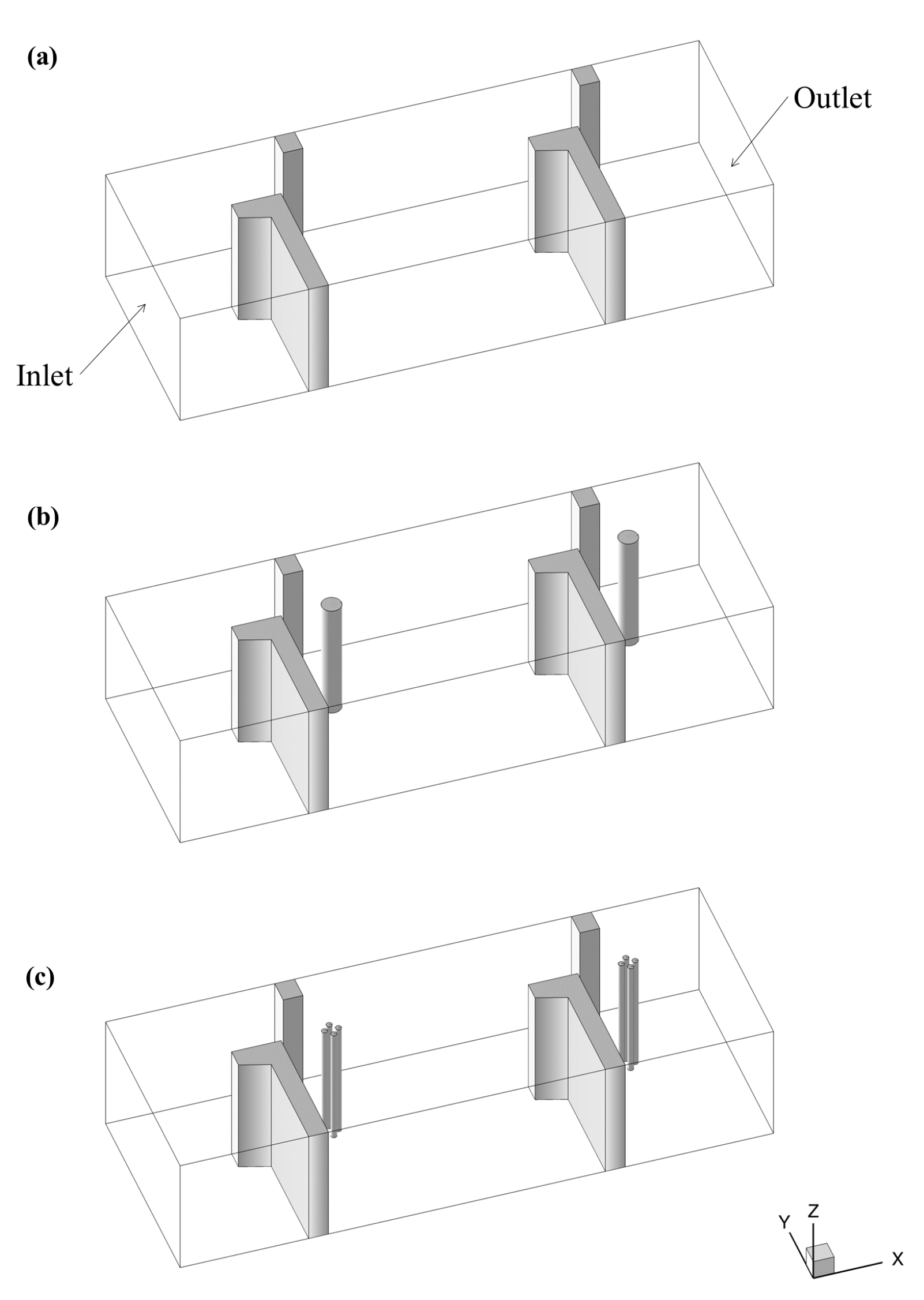
2.2. Computational Setup and Boundary Conditions

In the present numerical simulations, three scenarios were investigated to improve the hydraulic conditions for diadromous fishes swimming through the slots. The basic setup without supplementary cylinders corresponds to the VSF at the Arto-Blanca hydropower plant where extensive field measurements were conducted by Bombač et al. [26]. This fishway is comprised of 24 vertical slots and an acoustic Doppler velocimeter (ADV) was used to measure the velocity components in a selected pool in the downstream section. The layout of the selected pool is shown in Figure 1 with related geometric parameters. Each pool is of the same size with a length (L) of 3.0 m and a width (W) of 2.2 m. The flow conditions were kept constant during measurements, i.e., the discharge $Q=1.0$ m${}^3$/s and water depth $H=1.30$ m, indicating a fully developed stage has been achieved. Two gauging points along the main current and four sampling lines at the depth of z/H = 0.4 are represented by circles and dashed lines, respectively.

The vertical slot, located at the entrance of each pool, is formed by a long baffle on one side and a short baffle on the other side in the original design. The asymmetric layout is deliberately designed to create a wide resting cavity between two neighboring long baffles. Supplementary emergent cylinders are embedded downstream of the slots to separate the high-speed incoming flow in two different arrangements. The first arrangement is an isolated cylinder with the diameter of 0.2 m employed in the main route just downstream; the second one is a cluster of four cylinders with the diameter of 0.06 m at the same position. The slimmer cylinders are located at four edges of the periphery of the isolated cylinder in each pool. Figure 2 demonstrates the computational domains with distributions of obstacles for the three scenarios.

In order to save the computation cost for LESs, the length of computational domains is limited to 6 m, including a half pool upstream, a complete pool in the middle section and a half pool downstream. As the VSF flow is fully developed in the measured pool, periodic boundary conditions are applied in the streamwise direction, i.e., outflow from the outlet is reused as the inflow of the inlet. The continuous flow was driven by the component of gravitational acceleration parallel to the channel bed, based on the bed slope that is equal to the water surface slope from field measurements ($S_0$ = 0.0167). The free surface in LESs is assumed as a frictionless rigid lid since the Froude number ($F_r$ = 0.098) was less than 0.1, indicating that the influence of free-surface impacts is not significant [36,37]. The near-wall velocities of the other solid boundaries were treated with a no-slip condition using wall functions. The obstacles, including baffles and supplementary cylinders are mapped with IB points, on which the near-wall velocity is determined by viscosity and the IB method. The same grid size is adopted in the three spatial directions, i.e., dx = dy = dz = 0.01 m, approximately 17.1 Mio grid cells in total.

Table 1. Hydraulic conditions and computational details.

Case	${\mathbf{U}}_{\mathbf{0}}$ (m/s)	Re	Fr	No. of Cylinders	No. of IB Points
1	0.3497	349,700	0.098	0	1,013,004
2	0.3497	349,700	0.098	2	1,141,488
3	0.3497	349,700	0.098	8	1,052,220

provides a summary of the flow conditions and simulation parameters. The Reynolds number ($Re=\frac{U_{0}H}{\nu }$) is computed based on the mean velocity ($U_0=\frac{Q}{WH}$) and the water depth.

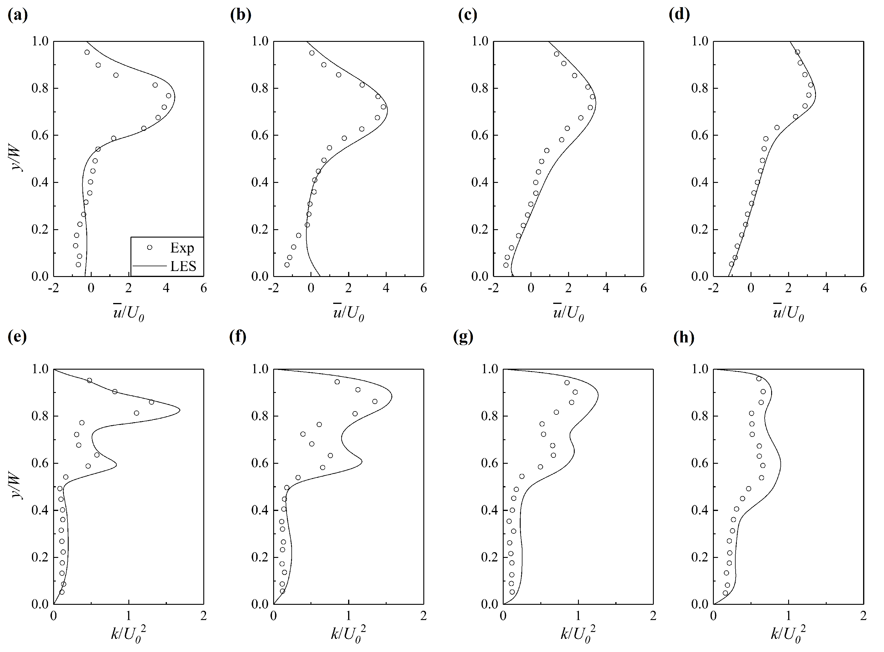
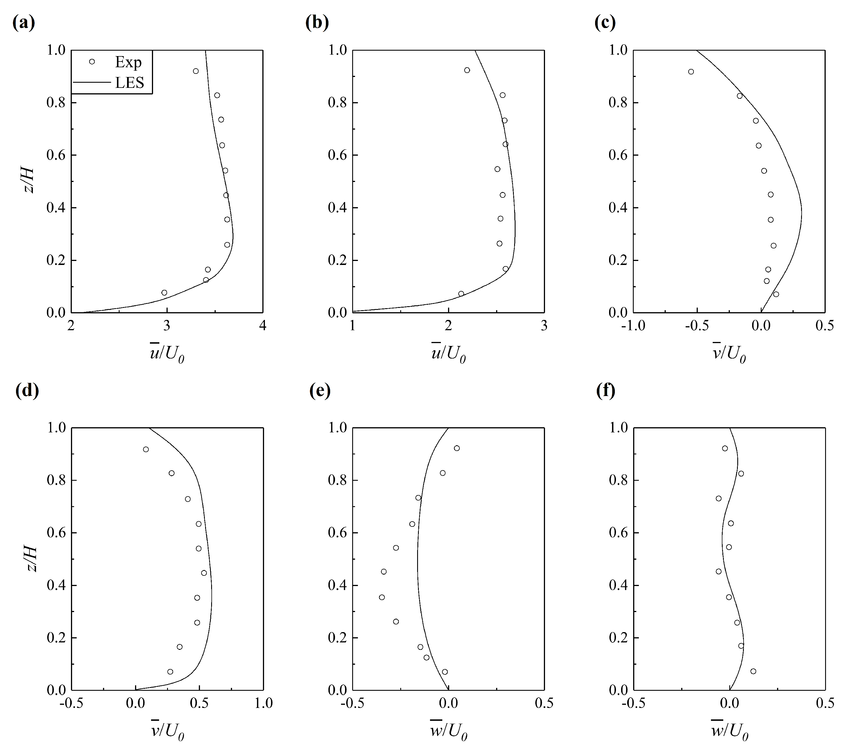
2.3. Model Validation

In this study, the simulation of the original case (Case 1) was performed for validation. The ADV experiment conducted by Bombač [26] was employed to validate the present numerical model. Figure 3 demonstrates the distributions of the time-averaged velocity normalized by the mean velocity along the streamwise ($\overline{u}/U_0$), the spanwise ($\overline{v}/U_0$) and the vertical ($\overline{v}/U_0$) directions. The gauging points V1 and V2 are located in the main stream and their velocity profiles are close to that of open-channel flow, generally accelerating from bed following a logarithmic law. The deceleration of the streamwise velocity near the water surface is caused by momentum transport due to the strong secondary flow in VSF, which is common in open-channel flow because of wall effects [38] or heterogeneity of bed roughness [28]. The comparison shows that the values of streamwise velocity predicted by LES are in good agreement with the experimental measurements, except at the top layer at the vicinity of the free surface, where the simulations overestimated the streamwise velocity by approximately 4% and 10% at V1 and V2, respectively. This is probably due to the difference between fluctuating free surface in situ measurements and the rigid-lid assumption adopted in the simulation. In addition, there is a small but consistent overestimation of the calculated streamwise velocity magnitude of approximately 8% to 12% within the middle layer (0.2 < z/H < 0.6) of velocity profile at V2.

It should be noted that the range of the x-axis is different based on the magnitude of velocity components. The velocity magnitude of V1 is markedly greater than that of V2 since V1 is located just downstream of the slot. The strong jet flow passes through V1 and subsequently decelerates before reaching V2. The secondary flow at V1 is stronger than that at V2 as well by comparison to spanwise velocity. The direction of spanwise flux is positive in the lower layer, but is negative in the upper layer at V1, which indicates a full secondary circulation. The spanwise velocity along the full profile at V2 is positive, i.e., flow here is diverted to the left bank for entering the next slot. The simulation successfully captures the property of spanwise velocity, but fails in providing equal precision compared to streamwise velocity. A dramatic overestimation of spanwise velocity magnitude is visible at 0.4 z/H at V1 in Figure 3c, where the peak value simulated is nearly 4 times of the peak measured value. A similar discrepancy also takes place at the same depth in Figure 3e for the predicted vertical velocity, which reaches 3.5 times the measured value. The agreement of spanwise and vertical velocity at V2 is relatively better than those at V1. The mean deviation rates of Figure 3d,e are reduced to approximately 32% and 13%, respectively.

Figure 4 compares calculated streamwise velocities and turbulent kinetic energy $k=0.5(\overline{u^{\prime }{u}^{\prime }}+\overline{v^{\prime }{v}^{\prime }}+\overline{w^{\prime }{w}^{\prime }})$ with measured data along the four spanwise gauging lines. The overall agreement between the measure velocity data and the LES results is remarkably good with mean deviation rate under 10%, expect velocity in the vicinity of the right wall (y/W < 0.2) along the gauging line S2. The predicted velocity varies around zero, which indicates the lower part of S2 is the interface of the corner vortex and the main vortex in the rest room, but the measured negative values proved that this near-wall region is occupied by the counter current of the main vortex. Moreover, LES overestimates the turbulent kinetic energy by approximately 23% based on the arithmetic mean of the four sampling lines, especially at the two peaks produced by the vortices downstream of the long and the short baffle, respectively. Nevertheless, the maximum deviation of the turbulent kinetic energy is limited under 35% and the varying pattern is captured well by LES along each line. The overall LES with the periodic boundary condition at the inlet and outlet is able to reproduce the fully developed flow field in the VSF.

3. Results and Discussion

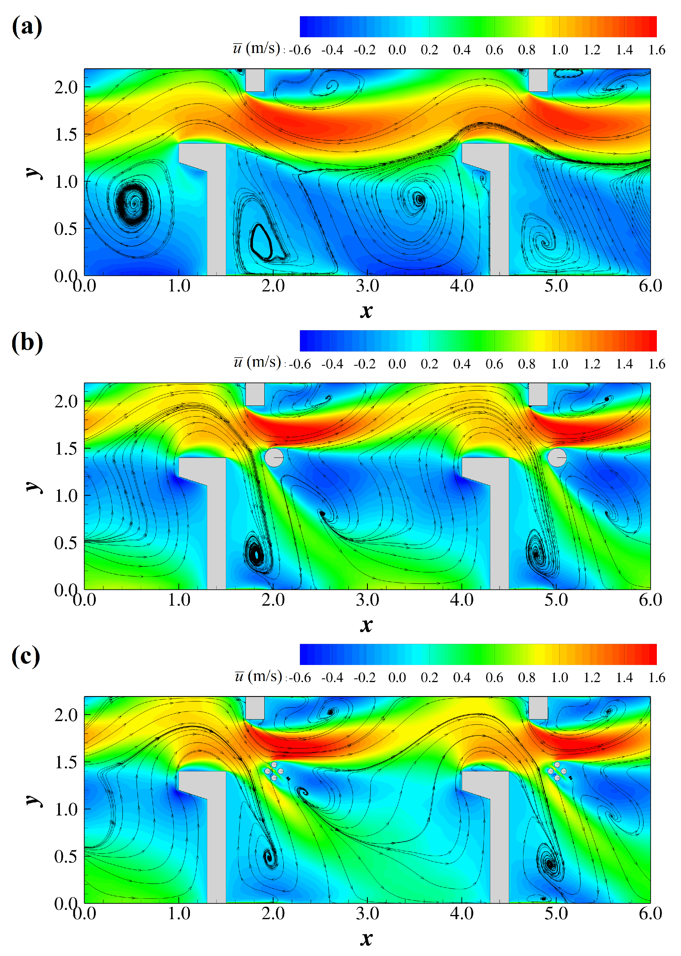
3.1. Time-Averaged Flow and Fish Swimming

Figure 5 presents the normalized time-averaged streamwise velocity with streamlines for the three cases. The horizontal planes are extracted at z/H = 0.5 for the representation of the whole water column. The color bar is deliberately adjusted to divide the velocity plane into three components: the red (and yellow) region of velocity ranging from 0.8 to 1.6 m/s denotes the major migration path, the green region of velocity ranging from 0.2 to 0.8 m/s denotes the minor migration path and the blue region of velocity ranging from −0.6 to 0.2 m/s denotes the recirculation zone.

As migratory fishes swim against the current, the positive values of velocity represent the reverse direction of fish motion. For the original design plotted in Figure 5a, the main stream passes through the consecutive slots as a curve jet and the maximum mean velocity with the value of 1.52 m/s takes place just downstream of the slot at the side of the short baffle. Most of the main current region is dominated by the major migration path with high momentum, which is within the swimming capacity for strong swimmers, such as adult Atlantic salmon [39], but is notably beyond weaker swimmers, such as Macquaria ambigua, Tandanus tandanus and juvenile Atlantic salmon [40,41]. The weak swimmers are able to swim upstream on the two low-speed minor migration paths attached to the major migration path on its two sides; however, the width of the two minor migration paths varies from approximately 0.05 m to 0.32 m, which is too narrow to be utilized. The weak swimmers have to overcome high-speed coming flow due to the limited width around the slot. The insertion of additional cylinders on the lower side of the slot significantly changes the flow field by dividing the original slot into two sub slots. The main current passes through the upper slot with approximately 8.5% and 9.6% amplification of the maximum streamwise velocity in Case 2 and Case 3, which remains in the range of strong fishes’ swimming capacity. The other branch flows through the lower slot and is significantly decelerated as the minor migration path and subsequently merges with the main current ahead of the next slot. Fishes with lower swimming preferences are able to take advantage of the slower coming flow in migration.

Two main recirculation regions are located at the two sides of the main current. The upper one is the wake of the short baffle with the length of 1.1 m, which is similar to the flow structure behind a spur dike. The main current reattaches the upper wall downstream of the small recirculation bubble and is subsequently obstructed by the next short baffle. The lower recirculation region occupies the whole pool between two long baffles, which is analogous to cavity flow with a small recirculation bubble in the left corner. This cavity between two long baffles could be employed as a resting room for migratory fishes, but the swirling flow may confuse migratory fishes with wrong upstream directions via their lateral lines [42]. The main vortex in the resting room is eliminated by the additional cylinders. Although the low-speed wake region of the isolated solid cylinder is notably larger than that of the porous cylinder cluster, the streamlines demonstrate that that uniformity of velocity in the rest room of Case 2 is greater than that of Case 3. The minor migration path created by the slim cylinders is filled with positive velocity contours, which creates a more favorable swimming environment for migratory fishes in sensing the right direction.

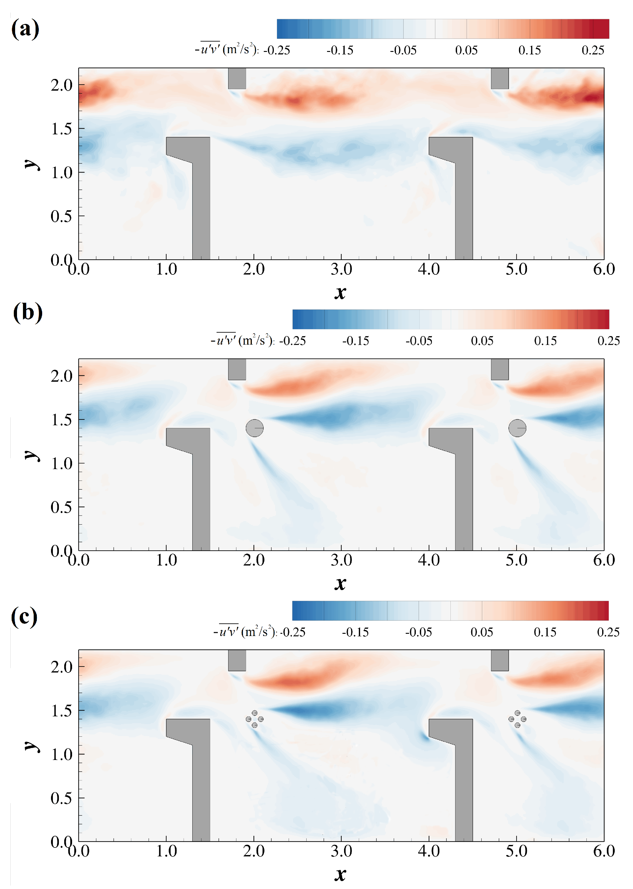
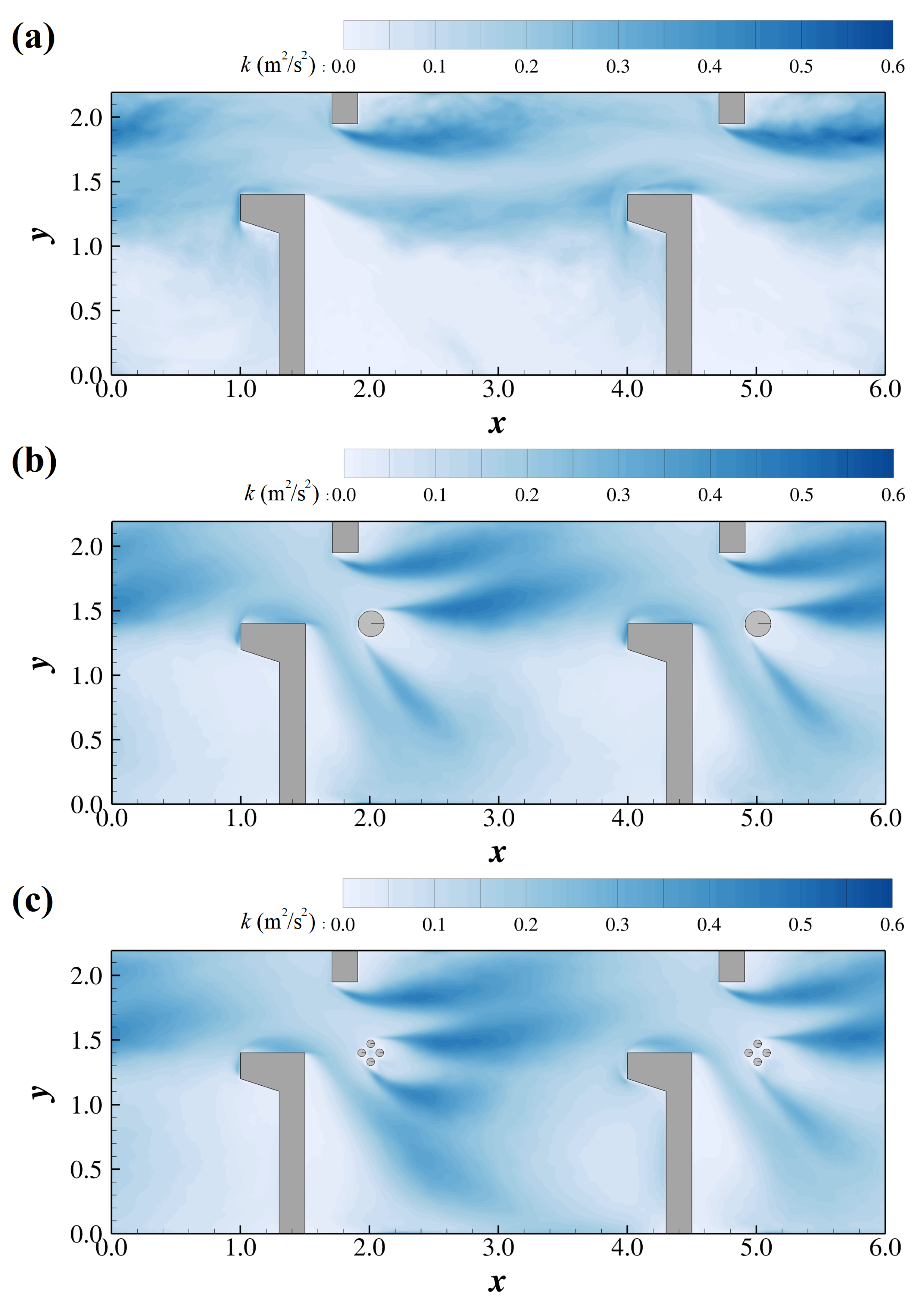
3.2. Second-Order Turbulence Statistics

Figure 6 compares the primary shear stress, $-\overline{u^{\prime }{v}^{\prime }}$, at z/H = 0.5 of the three cases, providing a view of the spatial distribution of turbulence in these cross sections. The areas of high primary shear stresses are emerged with strong fluid–solid interaction, including the wakes of baffles and cylinders. The primary shear stress, $-\overline{u^{\prime }{v}^{\prime }}$, is mainly produced due to velocity gradients of horizontal velocity components. In the original design depicted in Figure 6a, the maximum values of $-\overline{u^{\prime }{v}^{\prime }}$ are presented with the appearance of high-speed currents. The turbulence in the wake of the upper short baffle is more significant than that behind the long baffle because the velocity gradient is steeper due to the limited width of the cavity between the short baffles. As a result, high momentum and turbulence are concentrated in the narrow upper portion of the VSF, which is unfavorable for migratory fishes. Noteworthy, the core band inside the main stream is of pretty weak turbulence colored by white, i.e., it is a favorable path for large-bodies fishes with strong swimming capacity [43]. The turbulence level of the cavity between long baffles is relatively low as well, in which resting fish are free of the disturbance of vortices; however, resting fish needs to overcome the turbulence caused by the vortices shed from the edge of the long baffle when swimming back to the main stream. These velocity fluctuations could be weakened by optimization of the configuration of the baffles.

The insertion of the supplementary cylinders significantly alters the turbulence field of the horizontal plane. Asymmetric wake is produced due to the non-uniform jet flow from the slot. The intensity of the upper vortices is remarkably higher than that of the lower vortices. The peak value of the negative $-\overline{u^{\prime }{v}^{\prime }}$ caused by the upper vortices grows from −0.16 m${}^2$/s${}^2$ in Case 1, to −0.19 m${}^2$/s${}^2$ in Case 2 and finally reaches −0.21 m${}^2$/s${}^2$ in Case 3. Interestingly, the positive $-\overline{u^{\prime }{v}^{\prime }}$ due to the vortex shedding from the short baffle presents a different trend with the maximum value of 0.26, 0.17 and 0.19 m${}^2$/s${}^2$, respectively. Nevertheless, the path of weak turbulence remains with decreased width in the core region of the main stream. The supplementary cylinders also slightly increase the turbulence level in the resting room because of the vortex shedding on the lower side. It should be noted that the minor migration path in Case 3 is feathered with relatively low $-\overline{u^{\prime }{v}^{\prime }}$, which is friendly to small-bodied fishes [44].

The turbulence kinetic energy k is employed to quantify the turbulence intensity at the same plane in Figure 7. The characteristics of turbulence distribution are mainly in accordance with those of the primary shear stress. The areas of peak values are located in the wake of the short baffle and the supplementary cylinders, where coherent vortices are generated, propagated and dissipated. The polygonal heading of the long baffles separates the vortices upstream to inhibit the development of the turbulence. The growth of the mean turbulence kinetic energy along the minor migration path is approximately 120% and 140%, which normally increases the energy expenditure of fish swimming [43]. The turbulence kinetic energy around the cylinders of Case 3 is greater compared to that around the isolated cylinder of Case 2. The reason may be that the interaction of small-scale vortex shedding from small cylinders promotes the spanwise and vertical momentum exchange, which needs to be checked with 3-D flow structures.

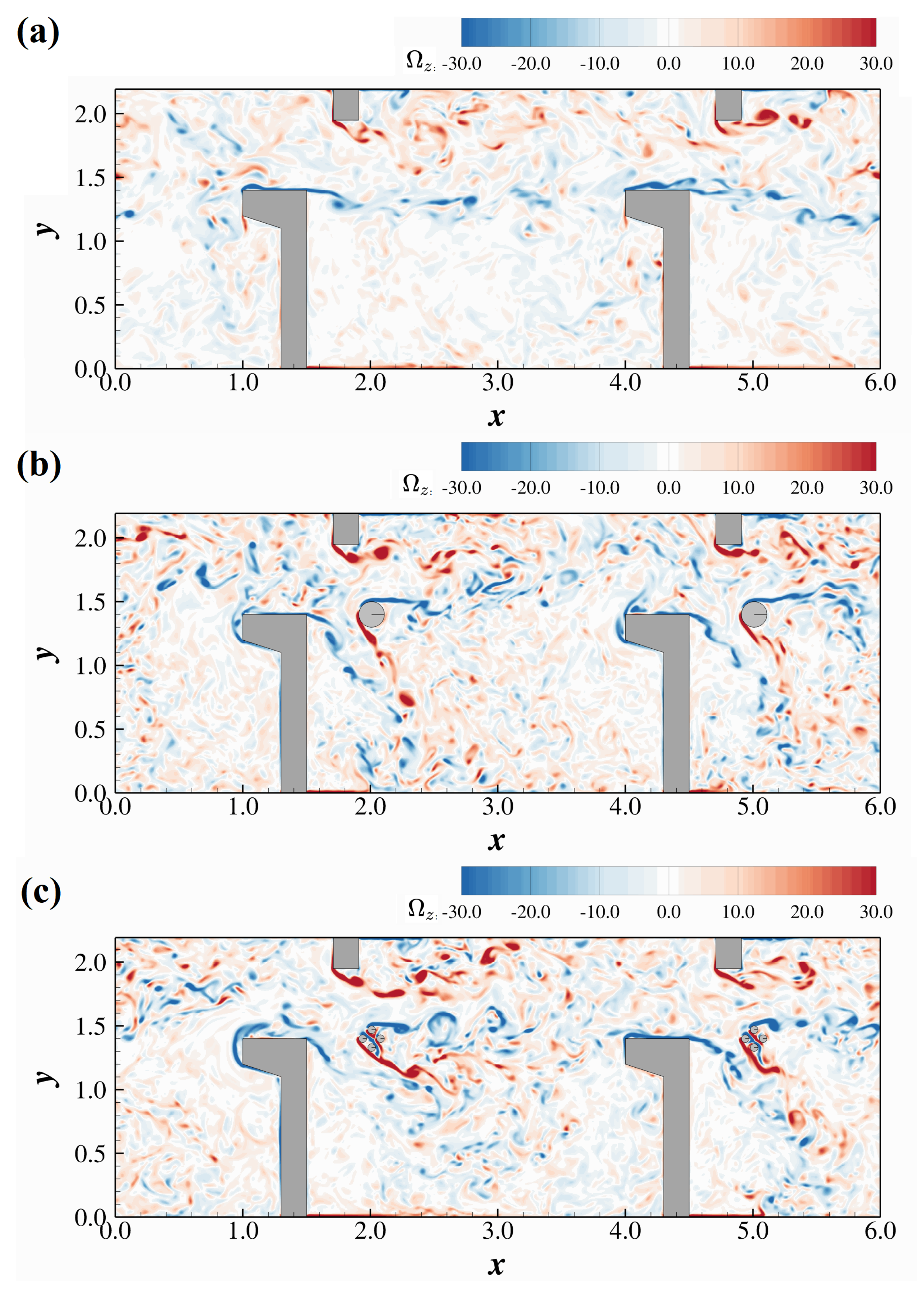
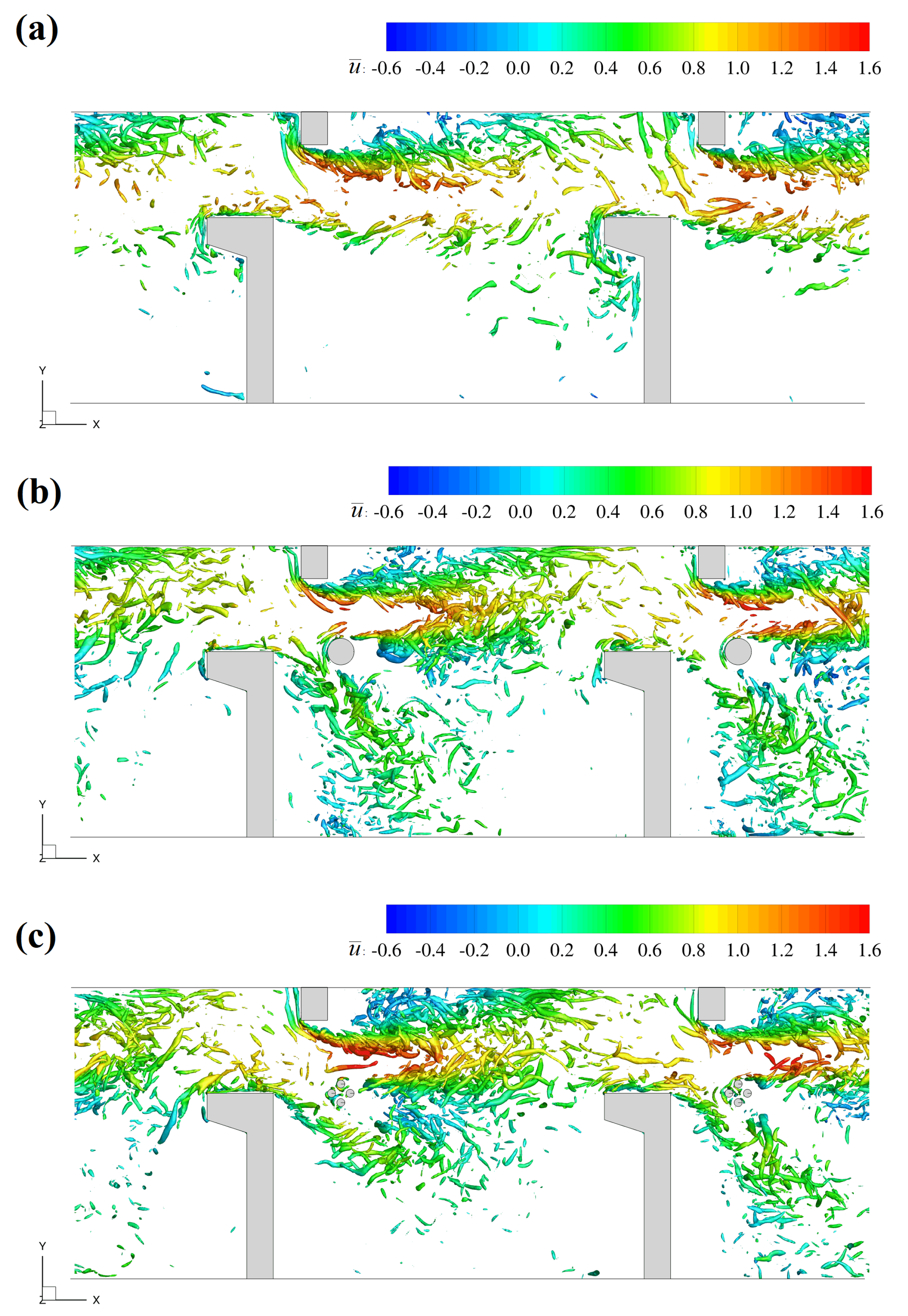
3.3. Instantaneous Flow Features

The flow field of VSF is featured by a wide spectrum of vortices and fish’s swimming capacity is remarkably influenced by eddy diameter, vorticity and orientation [45]. Figure 8 demonstrates the vertical vorticity, $\overline{{\Omega }_z}$, at the half-depth plane of the three cases. Vorticity is a hydrodynamic parameter quantifying how fast a region of fluid is spinning. Similar to the insertion of supplementary cylinders, shear layers are generated on the cylinder surface and separate into vortices of wakes. The transition from the shear layers to the generation of K-H vortices is asymmetrically distributed on the two sides of the isolated cylinder in Case 2 or the cylinder cluster in Case 3. The vortex shedding on the upper surface and lower surface are decorrelated, i.e., the onset of K-H vortices on the lower surface is much earlier than that on the upper surface. The separation of vortices on the outline of the cylinder cluster in Case 3 is delayed due to reduced block effects compared to the isolated cylinder in Case 2. As a result, the separated shear layer is transmitted to vortices in the forepart of the cavities and subsequently dissipated along the lower wall of the VSF in Case 2, while the transition and dissipation in Case 2 takes place in the middle section of the cavity. It should be noted that the vorticity around the short upper baffle is enhanced due to the influence of supplementary cylinders. The increase in vorticity can cause stability challenges for migratory fishes [46].

In order to better visualize the three dimensional vortex structures, Figure 9 shows the iso-surfaces of the Q criterion in the computational domain. The K-H instability developed by the transition of shear layers coming off the edge of the baffle and cylinder to smaller rollers is shown for the three cases. The rollers are mostly vertical in orientation, colored by the contours of time-averaged streamwise velocity for highlighting the kinetic energy carried by vortices. In Case 1, a broad spectrum of energetic vortices travels from the upper edge of the main current to the upper wall of the VSF similar to coherent structures around a spur dike. The other side of the main stream is distributed with sparse rollers with less momentum due to relatively weak shear stresses. The insertion of cylinders notably increases the amount of vortices depicted in Figure 9b,c; however, these vortices shed from cylinders are not as energetic as those around the short baffle, and thus fish swimming along the major migration path has to overcome stronger vortices while fish swimming along the minor migration path meets weaker eddies. On the other hand, hydraulic perturbation upon fish’s swimming stability is caused by vortices with a minimum diameter of 76% of the fish body length [46]. The influence of small eddies produced by the slim cylinders in Case 3 is not so significant as eddies produced by the thick solid cylinder in Case 2.

4. Conclusions

In this study, numerical experiments were carried out for optimization of an established VSF with supplementary cylinders. The method of LES was employed to elucidate and quantify the flow and associated turbulence structures in the VSF. Numerical setup and boundary conditions of Case 1 were chosen to reproduce fully developed flow conditions corresponding to the original design of the VSF. Field measurements at gauging points and lines were employed in validation and confirmation of the LES’ capability to accurately reproduce the flow field. Good agreement between LES and measured data is achieved both in time-averaged velocity and turbulent kinetic energy. The supplementary cylinders were inserted on the lower side of the main current in two different arrangements. An isolated thick cylinder was used in Case 2, whereas a cluster of four slim cylinders was utilized in Case 3. Flow properties at the half height of the three cases were extracted, presented and discussed with fish swimming. The horizontal plane of the VSF can be divided into a major migration path, minor migration paths and recirculation zones based on the range of time-averaged streamwise velocity. In the original design (Case 1), the main current through successive slots consisted of a major migration path and two minor migration paths; however, weak swimmers can hardly use the paths because the flow velocity of the major migration path is beyond their swimming capacity, which is normally under 0.8 m/s, and the width of the minor migration paths is too narrow, which is reduced to approximately 0.05 m at the slot. The supplementary cylinders solve the problem by separating a low-speed branch from the main current as a minor migration path with comparable width to the major one. The minor migration path of Case 3 was more favorable to migratory fishes in sensing the upstream direction because of the overall positive velocity along the route. The insertion of cylinders promotes the turbulence intensity based on the quantitative analysis of the primary shear stress and turbulence kinetic energy, which can produce extra energy expenditure for fish swimming. Moreover, the magnitude and area of vorticity is increased with the presence of supplementary cylinders as well, but the eddy diameter is not amplified to reach the critical value, 76% of fish body length, to influence the swimming stability. The vortices around the four slim cylinders in Case 2 were smaller in size and lower in momentum compared to those around the isolated cylinder in Case 3. The results numerically suggest that a porous cluster of slim cylinders outperforms an isolated solid cylinder in optimizing the VSF for fishes with lower swimming ability, and experimental studies with target fishes should be carried out before application to specific VSF engineering.

References

1. Nilsson, C.; Reidy, C.A.; Dynesius, M.; Revenga, C. Fragmentation and Flow Regulation of the World’s Large River Systems. Science 2005, 308, 405–408. [Google Scholar] [CrossRef] [PubMed] [Green Version]
2. Zarfl, C.; Lumsdon, A.E.; Berlekamp, J.; Tydecks, L.; Tockner, K. A global boom in hydropower dam construction. Aquat. Sci. 2015, 77, 161–170. [Google Scholar] [CrossRef]
3. Chen, S.; Chen, B.; Fath, B.D. Assessing the cumulative environmental impact of hydropower construction on river systems based on energy network model. Renew. Sustain. Energy Rev. 2015, 42, 78–92. [Google Scholar] [CrossRef]
4. Kuriqi, A.; Pinheiro, A.N.; Sordo-Ward, A.; Garrote, L. Influence of hydrologically based environmental flow methods on flow alteration and energy production in a run-of-river hydropower plant. J. Clean. Prod. 2019, 232, 1028–1042. [Google Scholar] [CrossRef]
5. Radinger, J.; Wolter, C. Patterns and predictors of fish dispersal in rivers. Fish Fish. 2014, 15, 456–473. [Google Scholar] [CrossRef]
6. Lynch, A.J.; Cooke, S.J.; Deines, A.M.; Bower, S.D.; Bunnell, D.B.; Cowx, I.G.; Nguyen, V.M.; Nohner, J.; Phouthavong, K.; Riley, B.; et al. The social, economic, and environmental importance of inland fish and fisheries. Environ. Rev. 2016, 24, 115–121. [Google Scholar] [CrossRef] [Green Version]
7. Wu, S.; Rajaratnam, N.; Katopodis, C. Structure of Flow in Vertical Slot Fishway. J. Hydraul. Eng. 1999, 125, 351–360. [Google Scholar] [CrossRef]
8. Rodriguez, T.T.; Agudo, J.P.; Mosquera, L.P.; González, E.P. Evaluating vertical-slot fishway designs in terms of fish swimming capabilities. Ecol. Eng. 2006, 27, 37–48. [Google Scholar] [CrossRef]
9. Thiem, J.; Binder, T.; Dumont, P.; Hatin, D.; Hatry, C.; Katopodis, C.; Stamplecoskie, K.; Cooke, S.J. Multispecies fish passage behaviour in a vertical slot fishway on the Richelieu River, Quebec, Canada. River Res. Appl. 2013, 29, 582–592. [Google Scholar] [CrossRef]
10. Rajaratnam, N.; Katopodis, C.; Solanki, S. New designs for vertical slot fishways. Can. J. Civ. Eng. 1992, 19, 402–414. [Google Scholar] [CrossRef]
11. Li, G.; Sun, S.; Liu, H.; Zheng, T. Schizothorax prenanti swimming behavior in response to different flow patterns in vertical slot fishways with different slot positions. Sci. Total Environ. 2021, 754, 142142. [Google Scholar] [CrossRef]
12. An, R.d.; Li, J.; Yi, W.m.; Mao, X. Hydraulics and swimming behavior of schizothorax prenanti in vertical slot fishways. J. Hydrodyn. 2019, 31, 169–176. [Google Scholar] [CrossRef]
13. Roscoe, D.W.; Hinch, S.G. Effectiveness monitoring of fish passage facilities: Historical trends, geographic patterns and future directions. Fish Fish. 2010, 11, 12–33. [Google Scholar] [CrossRef]
14. Tarrade, L.; Pineau, G.; Calluaud, D.; Texier, A.; David, L.; Larinier, M. Detailed experimental study of hydrodynamic turbulent flows generated in vertical slot fishways. Environ. Fluid Mech. 2011, 11, 1–21. [Google Scholar] [CrossRef] [Green Version]
15. Katopodis, C.; Williams, J.G. The development of fish passage research in a historical context. Ecol. Eng. 2012, 48, 8–18. [Google Scholar] [CrossRef]
16. Noonan, M.J.; Grant, J.W.A.; Jackson, C.D. A quantitative assessment of fish passage efficiency: Effectiveness of fish passage facilities. Fish Fish. 2012, 13, 450–464. [Google Scholar] [CrossRef]
17. Chorda, J.; Maubourguet, M.M.; Roux, H.; Larinier, M.; Tarrade, L.; David, L. Two-dimensional free surface flow numerical model for vertical slot fishways. J. Hydraul. Res. 2010, 48, 141–151. [Google Scholar] [CrossRef] [Green Version]
18. Tran, T.D.; Chorda, J.; Laurens, P.; Cassan, L. Modelling nature-like fishway flow around unsubmerged obstacles using a 2D shallow water model. Environ. Fluid Mech. 2016, 16, 413–428. [Google Scholar] [CrossRef] [Green Version]
19. Bombač, M.; Četina, M.; Novak, G. Study on flow characteristics in vertical slot fishways regarding slot layout optimization. Ecol. Eng. 2017, 107, 126–136. [Google Scholar] [CrossRef]
20. Quaresma, A.L.; Romão, F.; Branco, P.; Ferreira, M.T.; Pinheiro, A.N. Multi slot versus single slot pool-type fishways: A modelling approach to compare hydrodynamics. Ecol. Eng. 2018, 122, 197–206. [Google Scholar] [CrossRef]
21. Ahmadi, M.; Ghaderi, A.; MohammadNezhad, H.; Kuriqi, A.; Di Francesco, S. Numerical investigation of hydraulics in a vertical slot fishway with upgraded configurations. Water 2021, 13, 2711. [Google Scholar] [CrossRef]
22. Mitsopoulos, G.; Theodoropoulos, C.; Papadaki, C.; Dimitriou, E.; Santos, J.M.; Zogaris, S.; Stamou, A. Model-based ecological optimization of vertical slot fishways using macroinvertebrates and multispecies fish indicators. Ecol. Eng. 2020, 158, 106081. [Google Scholar] [CrossRef]
23. Calluaud, D.; Pineau, G.; Texier, A.; David, L. Modification of vertical slot fishway flow with a supplementary cylinder. J. Hydraul. Res. 2014, 52, 614–629. [Google Scholar] [CrossRef]
24. Fuentes-Pérez, J.F.; Silva, A.T.; Tuhtan, J.A.; García-Vega, A.; Carbonell-Baeza, R.; Musall, M.; Kruusmaa, M. 3D modelling of non-uniform and turbulent flow in vertical slot fishways. Environ. Model. Softw. 2018, 99, 156–169. [Google Scholar] [CrossRef]
25. Chanson, H. Utilising the boundary layer to help restore the connectivity of fish habitats and populations. An engineering discussion. Ecol. Eng. 2019, 141, 105613. [Google Scholar] [CrossRef]
26. Bombač, M.; Novak, G.; Mlačnik, J.; Četina, M. Extensive field measurements of flow in vertical slot fishway as data for validation of numerical simulations. Ecol. Eng. 2015, 84, 476–484. [Google Scholar] [CrossRef]
27. Stoesser, T.; Kim, S.J.; Diplas, P. Turbulent flow through idealized emergent vegetation. J. Hydraul. Eng. 2010, 136, 1003–1017. [Google Scholar] [CrossRef]
28. Stoesser, T.; McSherry, R.; Fraga, B. Secondary currents and turbulence over a non-uniformly roughened open-channel bed. Water 2015, 7, 4896–4913. [Google Scholar] [CrossRef] [Green Version]
29. Gong, Y.; Stoesser, T.; Mao, J.; McSherry, R. LES of flow through and around a finite patch of thin plates. Water Resour. Res. 2019, 55, 7587–7605. [Google Scholar] [CrossRef] [Green Version]
30. Vui Chua, K.; Fraga, B.; Stoesser, T.; Ho Hong, S.; Sturm, T. Effect of bridge abutment length on turbulence structure and flow through the opening. J. Hydraul. Eng. 2019, 145, 04019024. [Google Scholar] [CrossRef]
31. Liu, Y.; Stoesser, T.; Fang, H. Effect of secondary currents on the flow and turbulence in partially filled pipes. J. Fluid Mech. 2022, 938. [Google Scholar] [CrossRef]
32. Liu, Y.; Stoesser, T.; Fang, H. Impact of turbulence and secondary flow on the water surface in partially filled pipes. Phys. Fluids 2022, 34, 035123. [Google Scholar] [CrossRef]
33. Uhlmann, M. An immersed boundary method with direct forcing for the simulation of particulate flows. J. Comput. Phys. 2005, 209, 448–476. [Google Scholar] [CrossRef] [Green Version]
34. Cristallo, A.; Verzicco, R. Combined immersed boundary/large-eddy-simulations of incompressible three dimensional complex flows. Flow Turbul. Combust. 2006, 77, 3–26. [Google Scholar] [CrossRef]
35. Smagorinsky, J. General circulation experiments with the primitive equations: I. The basic experiment. Mon. Weather. Rev. 1963, 91, 99–164. [Google Scholar] [CrossRef]
36. Bomminayuni, S.; Stoesser, T. Turbulence statistics in an open-channel flow over a rough bed. J. Hydraul. Eng. 2011, 137, 1347–1358. [Google Scholar] [CrossRef]
37. Ouro, P.; Wilson, C.A.M.E.; Evans, P.; Angeloudis, A. Large-eddy simulation of shallow turbulent wakes behind a conical island. Phys. Fluids 2017, 29, 126601. [Google Scholar] [CrossRef] [Green Version]
38. Rodríguez, J.F.; García, M.H. Laboratory measurements of 3-D flow patterns and turbulence in straight open channel with rough bed. J. Hydraul. Res. 2008, 46, 454–465. [Google Scholar] [CrossRef]
39. Thorstad, E.B.; ØKland, F.; Finstad, B. Effects of telemetry transmitters on swimming performance of adult Atlantic salmon. J. Fish Biol. 2000, 57, 531–535. [Google Scholar] [CrossRef]
40. Watson, J.R.; Goodrich, H.R.; Cramp, R.L.; Gordos, M.A.; Franklin, C.E. Utilising the boundary layer to help restore the connectivity of fish habitats and populations. Ecol. Eng. 2018, 122, 286–294. [Google Scholar] [CrossRef]
41. Lacroix, G.L.; Knox, D.; McCurdy, P. Effects of implanted acoustic transmitters on juvenile Atlantic salmon. Trans. Am. Fish. Soc. 2004, 133, 211–220. [Google Scholar] [CrossRef]
42. Bleckmann, H.; Zelick, R. Lateral line system of fish. Integr. Zool. 2009, 4, 13–25. [Google Scholar] [CrossRef]
43. Lacey, R.J.; Neary, V.S.; Liao, J.C.; Enders, E.C.; Tritico, H.M. The IPOS framework: Linking fish swimming performance in altered flows from laboratory experiments to rivers. River Res. Appl. 2012, 28, 429–443. [Google Scholar] [CrossRef]
44. Wilkes, M.; Enders, E.; Silva, A.; Acreman, M.; Maddock, I. Position choice and swimming costs of juvenile Atlantic salmon salmo salar in turbulent flow. J. Ecohydraulics 2017, 2, 16–27. [Google Scholar] [CrossRef]
45. Cote, A.J.; Webb, P.W. Living in a Turbulent World—A New Conceptual Framework for the Interactions of Fish and Eddies. Integr. Comp. Biol. 2015, 55, 662–672. [Google Scholar] [CrossRef] [Green Version]
46. Tritico, H.M.; Cotel, A.J. The effects of turbulent eddies on the stability and critical swimming speed of creek chub (Semotilus atromaculatus). J. Exp. Biol. 2010, 213, 2284–2293. [Google Scholar] [CrossRef] [Green Version]
Figure 1. Plane layout for the selected pool of the VSF with geometric parameters. V1 and V2 are two ADV gauging points. S1 to S4 denote the four sampling lines.
Water 14 01772 g001
Figure 2. A 3D view of the computation domains with obstacles of three cases. (a) Case 1: original design; (b) Case 2: an isolated cylinder in each pool; (c) Case 3: four cylinders in each pool.
Water 14 01772 g002
Figure 3. Measured and computed vertical profiles of normalized time-averaged velocity of (a) streamwise component at V1; (b) streamwise component at V2; (c) spanwise component at V1; (d) spanwise component at V2; (e) vertical component at V1; (f) spanwise component at V2.
Water 14 01772 g003
Figure 4. Measured and computed of normalized data along sampling lines: (ad) normalized streamwise time-averaged velocity; (eh) normalized turbulent kinetic energy.
Water 14 01772 g004
Figure 5. Distributions of time-averaged streamwise velocity with streamlines at the half height of: (a) Case1; (b) Case 2; (c) Case 3.
Water 14 01772 g005
Figure 6. Contours of primary shear stress in a the horizontal plane at the half height of: (a) Case 1; (b) Case 2; (c) Case 3.
Water 14 01772 g006
Figure 7. Contours of turbulence kinetic energy in a the horizontal plane at the half height of: (a) Case 1; (b) Case 2; (c) Case 3.
Water 14 01772 g007
Figure 8. Contours of turbulence kinetic energy in a the horizontal plane at half height of: (a) Case 1; (b) Case 2; (c) Case 3.
Water 14 01772 g008
Figure 9. Visualization of the coherent structures using the Q criterion colored by time-averaged streamwise velocity: (a) Case 1; (b) Case 2; (c) Case 3.
Water 14 01772 g009