
Correction of ERA5 Wind for Regional Climate Projections of Sea Waves

 ,
,  ,
,  and
and 
Abstract
1. Introduction
2. Datasets and Methods
2.1. Wind and Wave Observations
2.2. ERA5 Reanalysis
2.3. COSMO-CLM Regional Climate Model
2.4. Spectral Wave Modeling
2.5. Climatological Constraint Condition for ERA5 Sea Wind
3. Model Assessment
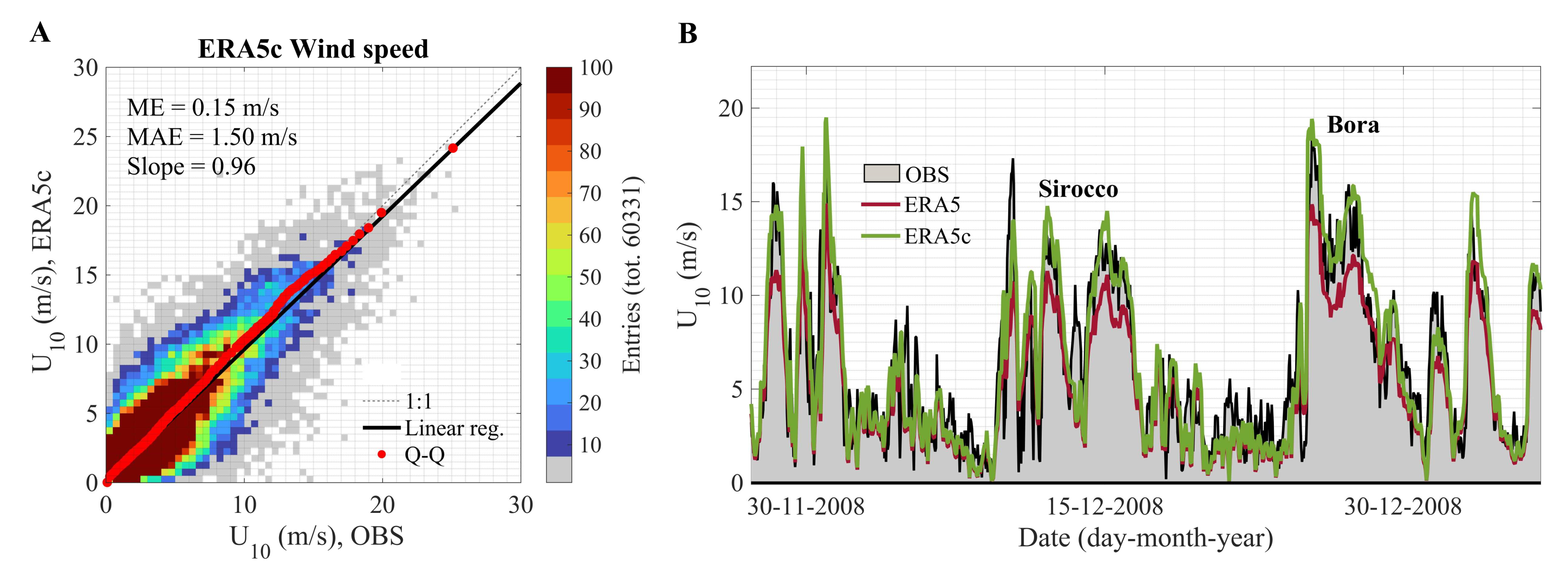
3.1. ERA5 Wind
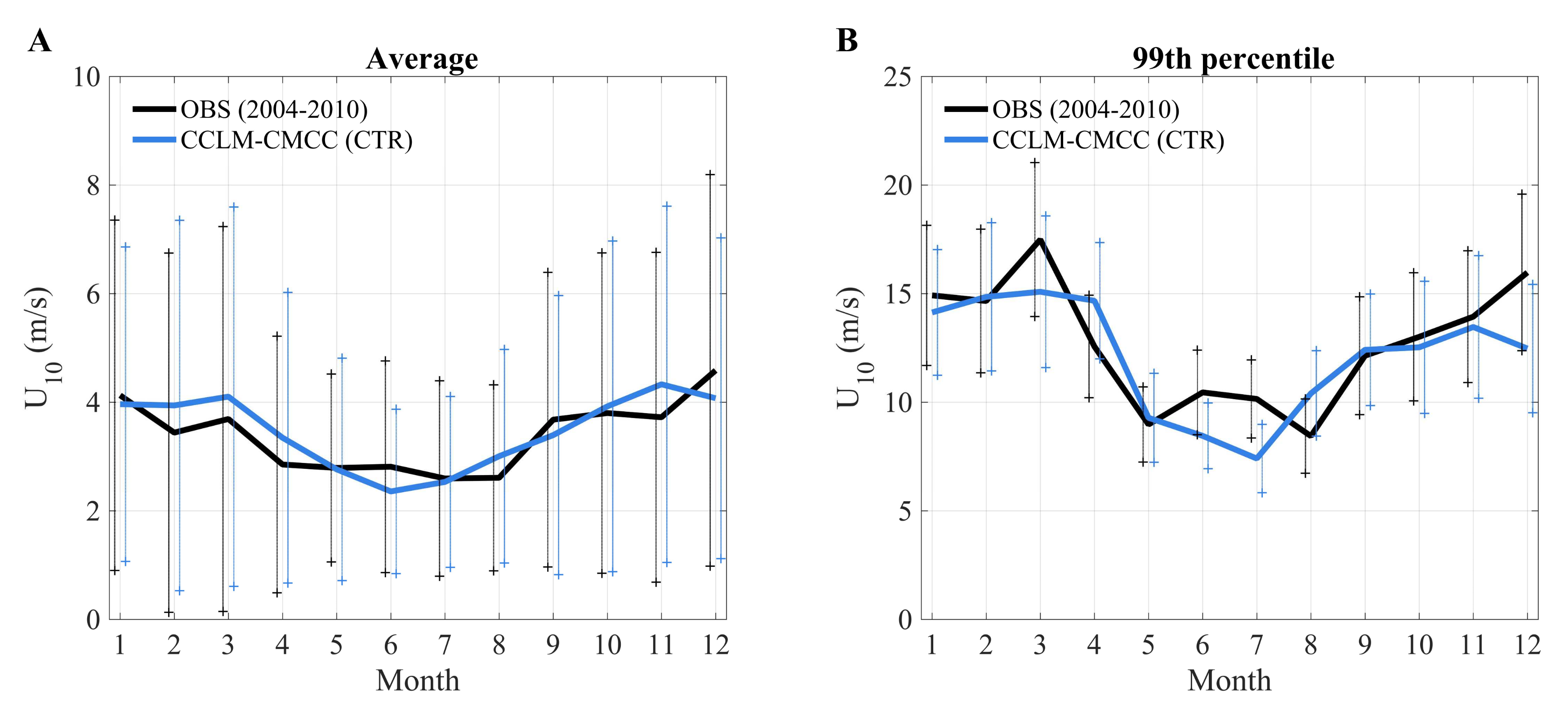
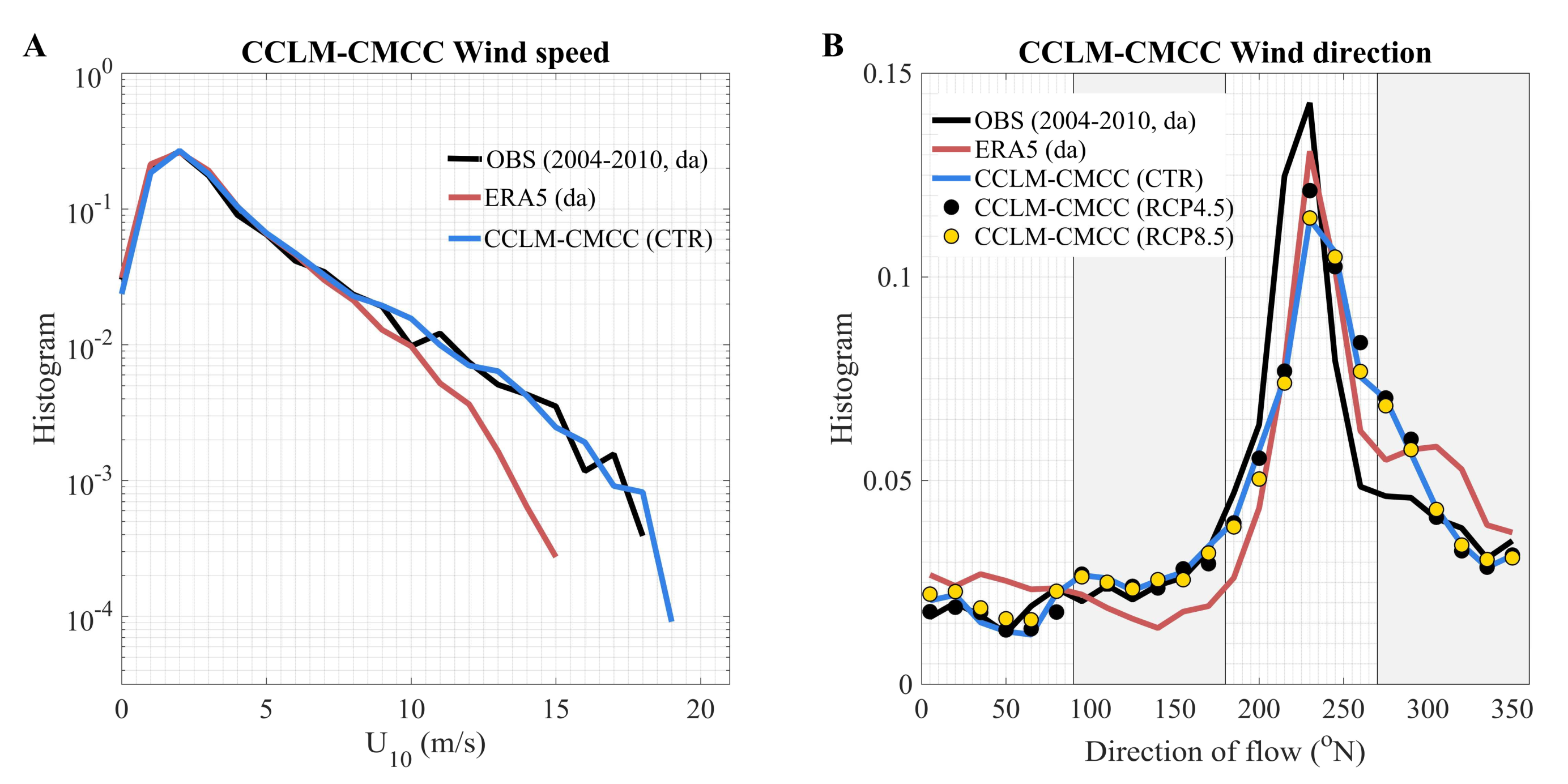
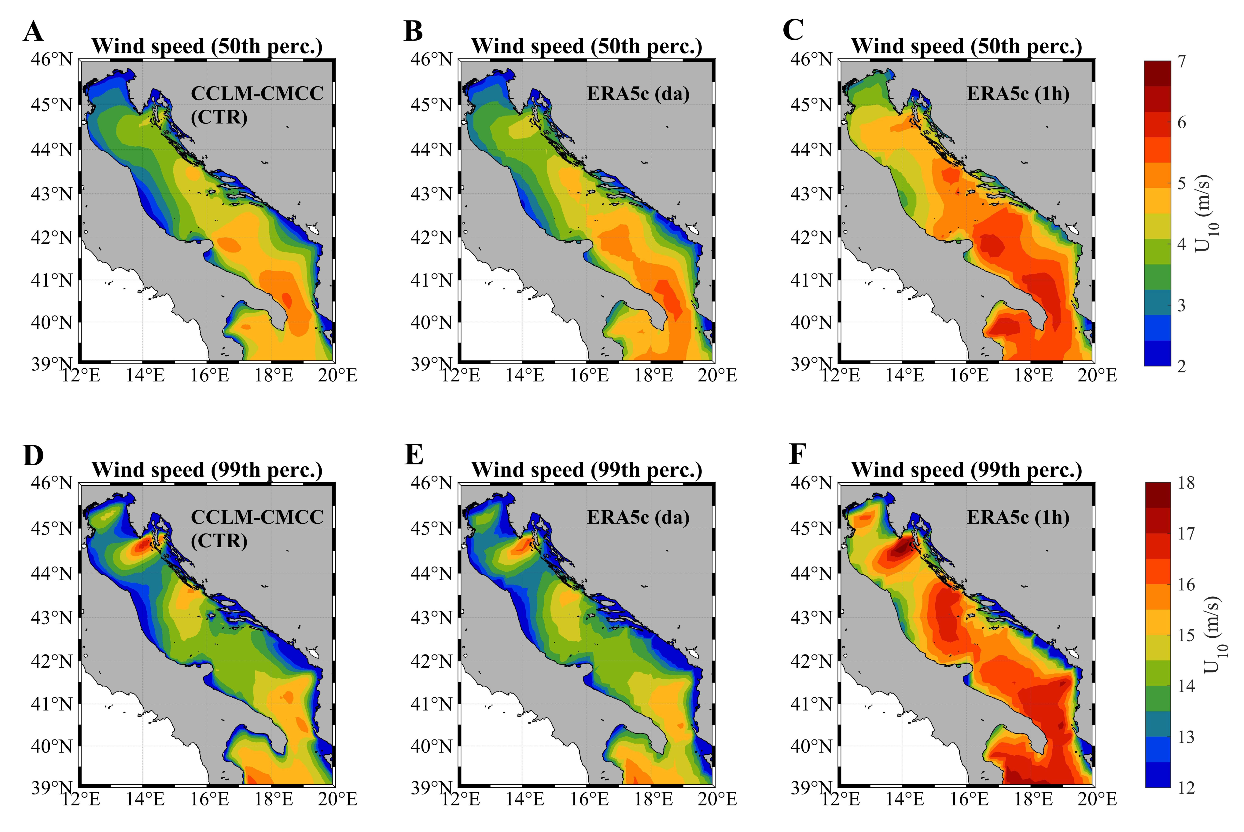
3.2. CCLM-CMCC Wind
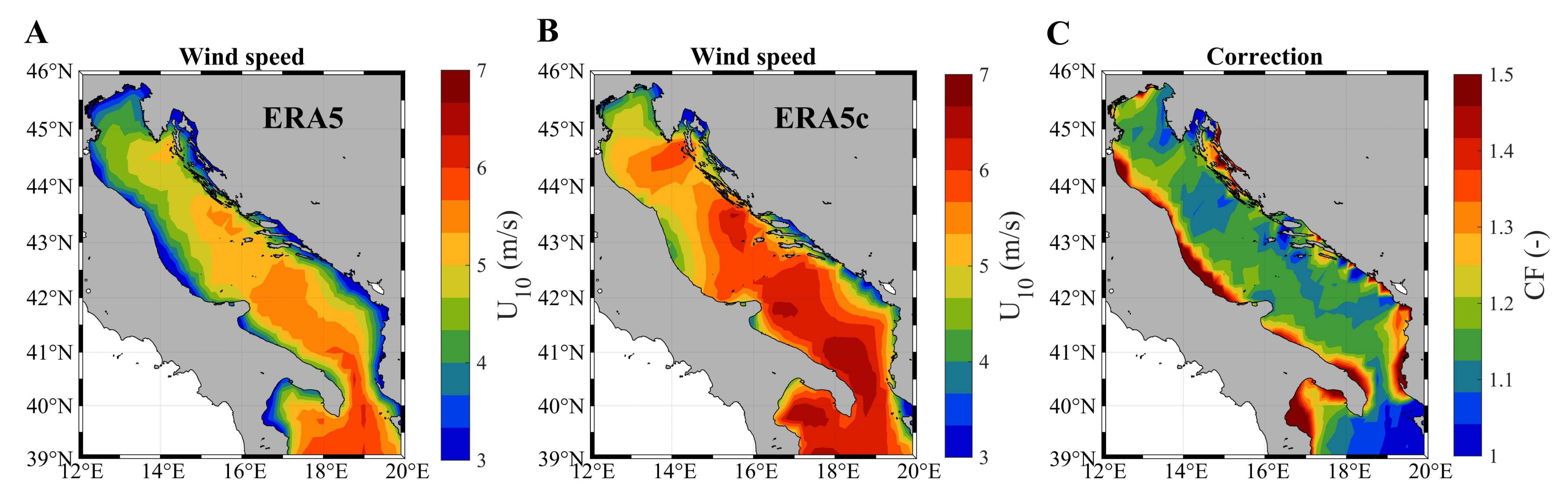
3.3. ERA5c Wind
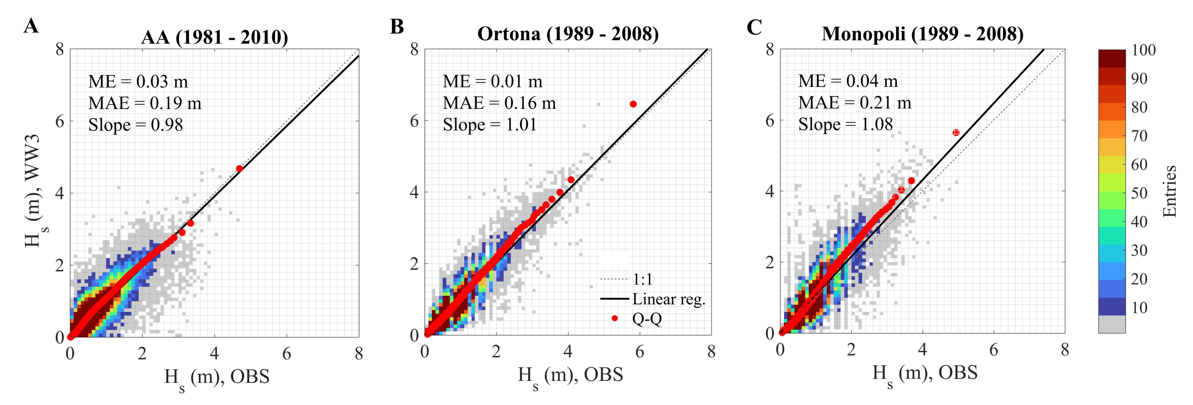
3.4. Waves
4. Application to Wave Climate Scenarios over the Adriatic Sea
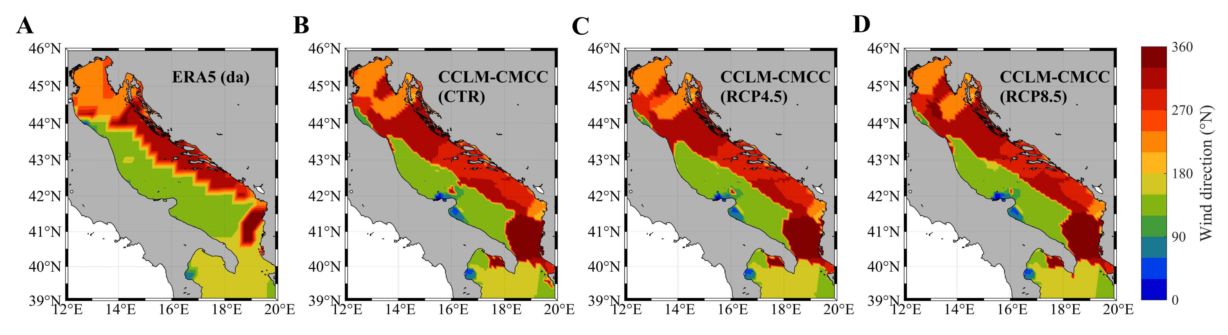
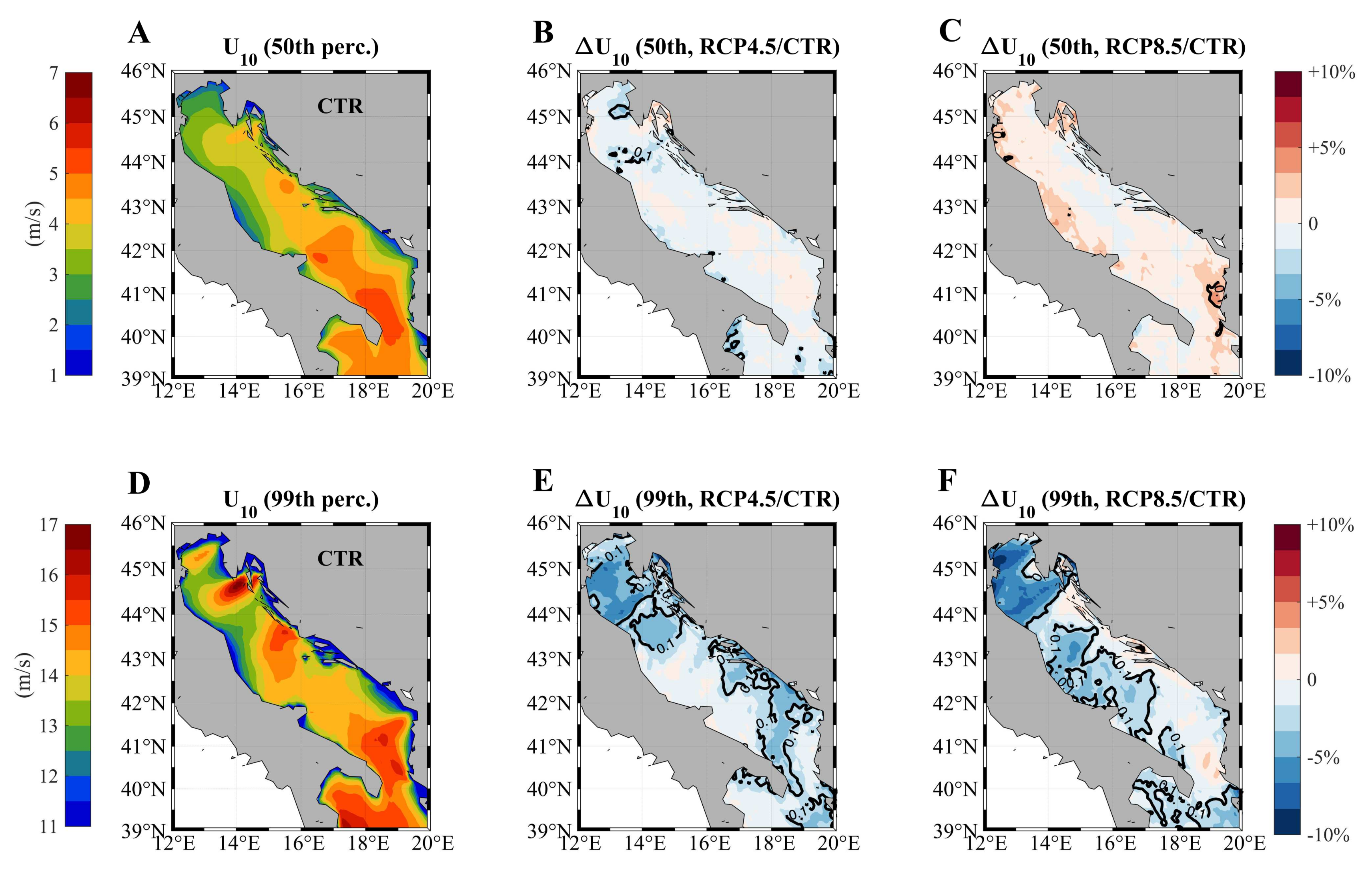
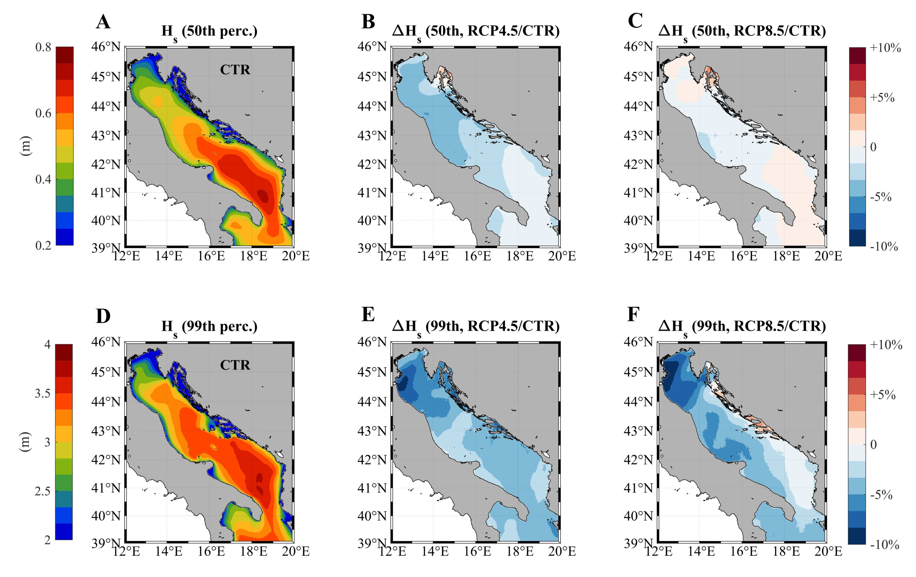
4.1. Basin Scale Analysis
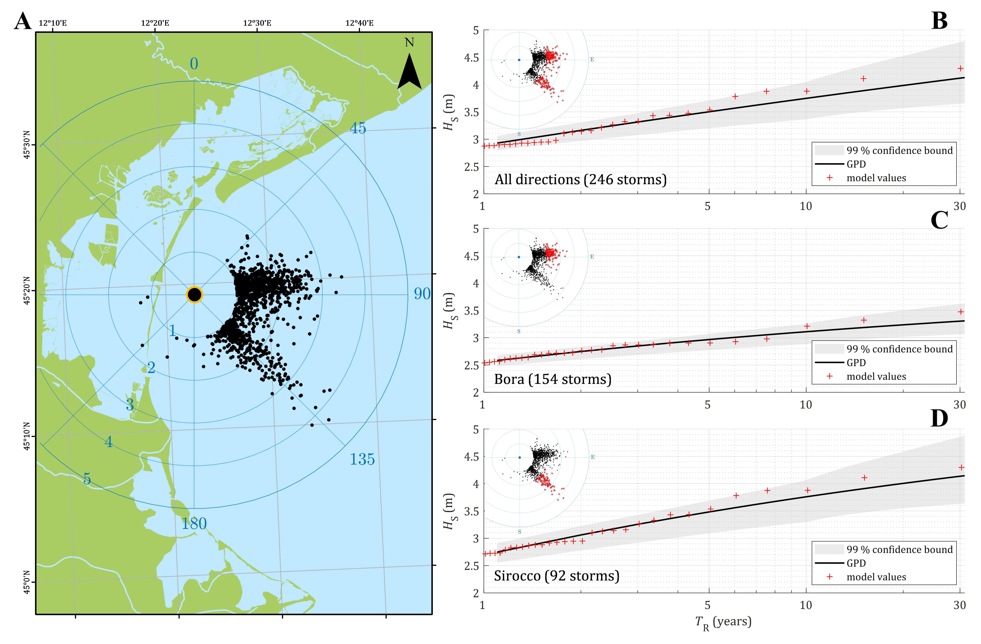
4.2. Extreme Value Analysis Offshore Venice (Italy)
5. Concluding Remarks
Author Contributions
Funding
Institutional Review Board Statement
Data Availability Statement
Acknowledgments
Conflicts of Interest
References
- Cavaleri, L.; Fox-Kemper, B.; Hemer, M. Wind Waves in the Coupled Climate System. Bull. Am. Meteorol. Soc. 2012, 93, 1651–1661. [Google Scholar] [CrossRef]
- Bitner-Gregersen, E.M.; Cramer, E.H.; Løseth, R. Uncertainties of load characteristics and fatigue damage of ship structures. Mar. Struct. 1995, 8, 97–117. [Google Scholar] [CrossRef]
- Hansom, J.D.; Switzer, A.D.; Pile, J. Chapter 11—Extreme Waves: Causes, Characteristics, and Impact on Coastal Environments and Society. In Coastal and Marine Hazards, Risks, and Disasters; Shroder, J.F., Ellis, J.T., Sherman, D.J., Eds.; Hazards and Disasters Series; Elsevier: Boston, MA, USA, 2015; pp. 307–334. ISBN 978-0-12-396483-0. [Google Scholar]
- Oppenheimer, M.; Glavovic, B.C.; Hinkel, J.; van de Wal, R.; Magnan, A.K.; Abd-Elgawad, A.; Cai, R.; Cifuentes-Jara, M.; DeConto, R.M.; Ghosh, T.; et al. Sea Level Rise and Implications for Low-Lying Islands, Coasts and Communities. In IPCC Special Report on the Ocean and Cryosphere in a Changing Climate; Pörtner, H.-O., Roberts, D.C., Masson-Delmotte, V., Zhai, P., Tignor, M., Poloczanska, E., Eds.; Cambridge University Press: Cambridge, UK; New York, NY, USA, 2019; pp. 321–445. [Google Scholar] [CrossRef]
- Kalnay, E.; Kanamitsu, M.; Kistler, R.; Collins, W.; Deaven, D.; Gandin, L.; Iredell, M.; Saha, S.; White, G.; Woollen, J.; et al. The NCEP/NCAR 40-Year Reanalysis Project. Bull. Am. Meteorol. Soc. 1996, 77, 437–472. [Google Scholar] [CrossRef]
- Hersbach, H.; Bell, B.; Berrisford, P.; Hirahara, S.; Horányi, A.; Muñoz-Sabater, J.; Nicolas, J.; Peubey, C.; Radu, R.; Schepers, D.; et al. The ERA5 global reanalysis. Q. J. R. Meteorol. Soc. 2020, 146, 1999–2049. [Google Scholar] [CrossRef]
- Copernicus Climate Change Service (C3S) ERA5: Fifth Generation of ECMWF Atmospheric Reanalyses of the Global Climate. Copernicus Climate Change Serv. Climate Data Store (CDS). Available online: https://cds.climate.copernicus.eu/#!/search?text=ERA5&type=dataset (accessed on 22 April 2022).
- Coperncius Climate Bulletins. Available online: https://climate.copernicus.eu/climate-bulletins?q=monthly-maps-and-charts (accessed on 22 April 2022).
- Cucchi, M.; Weedon, G.P.; Amici, A.; Bellouin, N.; Lange, S.; Müller Schmied, H.; Hersbach, H.; Buontempo, C. WFDE5: Bias-adjusted ERA5 reanalysis data for impact studies. Earth Syst. Sci. Data 2020, 12, 2097–2120. [Google Scholar] [CrossRef]
- Bidlot, J.; Lemos, G.; Semedo, A. ERA5 Reanalysis and ERA5-Based Ocean Wave Hindcast; Coperncius Climate: Reading, UK, 2019. [Google Scholar]
- Von Schuckmann, K.; Le Traon, P.-Y.; Smith, N.; Pascual, A.; Djavidnia, S.; Gattuso, J.-P.; Grégoire, M.; Aaboe, S.; Alari, V.; Alexander, B.E.; et al. Copernicus Marine Service Ocean State Report, Issue 5. J. Oper. Oceanogr. 2021, 14, 1–185. [Google Scholar] [CrossRef]
- Barbariol, F.; Davison, S.; Falcieri, F.M.; Ferretti, R.; Ricchi, A.; Sclavo, M.; Benetazzo, A. Wind Waves in the Mediterranean Sea: An ERA5 Reanalysis Wind-Based Climatology. Front. Mar. Sci. 2021, 8, 760614. [Google Scholar] [CrossRef]
- Vannucchi, V.; Taddei, S.; Capecchi, V.; Bendoni, M.; Brandini, C. Dynamical Downscaling of ERA5 Data on the North-Western Mediterranean Sea: From Atmosphere to High-Resolution Coastal Wave Climate. J. Mar. Sci. Eng. 2021, 9, 208. [Google Scholar] [CrossRef]
- Dickinson, R.; Errico, R.; Giorgi, F.; Bates, G. A regional climate model for the western United States. Clim. Chang. 1989, 15, 383–422. [Google Scholar] [CrossRef]
- Giorgi, F. Thirty Years of Regional Climate Modeling: Where Are We and Where Are We Going next? J. Geophys. Res. Atmos. 2019, 124, 5696–5723. [Google Scholar] [CrossRef]
- Jacob, D.; Petersen, J.; Eggert, B.; Alias, A.; Christensen, O.B.; Bouwer, L.M.; Braun, A.; Colette, A.; Déqué, M.; Georgievski, G.; et al. EURO-CORDEX: New high-resolution climate change projections for European impact research. Reg. Environ. Chang. 2014, 14, 563–578. [Google Scholar] [CrossRef]
- Morim, J.; Hemer, M.; Wang, X.L.; Cartwright, N.; Trenham, C.; Semedo, A.; Young, I.; Bricheno, L.; Camus, P.; Casas-Prat, M.; et al. Robustness and uncertainties in global multivariate wind-wave climate projections. Nat. Clim. Chang. 2019, 9, 711–718. [Google Scholar] [CrossRef]
- Hemer, M.A.; Fan, Y.; Mori, N.; Semedo, A.; Wang, X.L. Projected changes in wave climate from a multi-model ensemble. Nat. Clim. Chang. 2013, 3, 471–476. [Google Scholar] [CrossRef]
- Colette, A.; Vautard, R.; Vrac, M. Regional climate downscaling with prior statistical correction of the global climate forcing. Geophys. Res. Lett. 2012, 39, L13707. [Google Scholar] [CrossRef]
- Wood, A.W.; Leung, L.R.; Sridhar, V.; Lettenmaier, D.P. Hydrologic Implications of Dynamical and Statistical Approaches to Downscaling Climate Model Outputs. Clim. Chang. 2004, 62, 189–216. [Google Scholar] [CrossRef]
- Deque, M. Frequency of precipitation and temperature extremes over France in an anthropogenic scenario: Model results and statistical correction according to observed values. Glob. Planet. Chang. 2007, 57, 16–26. [Google Scholar] [CrossRef]
- Li, D.; Feng, J.; Xu, Z.; Yin, B.; Shi, H.; Qi, J. Statistical Bias Correction for Simulated Wind Speeds Over CORDEX-East Asia. Earth Sp. Sci. 2019, 6, 200–211. [Google Scholar] [CrossRef]
- Michelangeli, P.-A.; Vrac, M.; Loukos, H. Probabilistic downscaling approaches: Application to wind cumulative distribution functions. Geophys. Res. Lett. 2009, 36, L11708. [Google Scholar] [CrossRef]
- Lobeto, H.; Menendez, M.; Losada, I.J. Future behavior of wind wave extremes due to climate change. Sci. Rep. 2021, 11, 7869. [Google Scholar] [CrossRef]
- Parker, K.; Hill, D.F. Evaluation of bias correction methods for wave modeling output. Ocean Model. 2017, 110, 52–65. [Google Scholar] [CrossRef]
- Intergovernmental Panel on Climate Change. Contribution of Working Groups I, II and III to the Fifth Assessment Report of the Intergovernmental Panel on Climate Change; Pachauri, R.K., Meyer, L.A., Eds.; Climate Change 2014: Synthesis Report; IPCC: Geneva, Switzerland, 2014. [Google Scholar]
- Signell, R.P.; Carniel, S.; Cavaleri, L.; Chiggiato, J.; Doyle, J.D.; Pullen, J.; Sclavo, M. Assessment of wind quality for oceanographic modelling in semi-enclosed basins. J. Mar. Syst. 2005, 53, 217–233. [Google Scholar] [CrossRef]
- Cushman-Roisin, B.; Gačić, M.; Poulain, P.-M.; Artegiani, A. (Eds.) Physical Oceanography of the Adriatic Sea; Springer: Dordrecht, The Netherlands, 2001; ISBN 978-90-481-5921-5. [Google Scholar]
- Lionello, P.; Cavaleri, L.; Nissen, K.M.; Pino, C.; Raicich, F.; Ulbrich, U. Severe marine storms in the Northern Adriatic: Characteristics and trends. Phys. Chem. Earth Parts A/B/C 2012, 40–41, 93–105. [Google Scholar] [CrossRef]
- Bucchignani, E.; Montesarchio, M.; Zollo, A.L.; Mercogliano, P. High-resolution climate simulations with COSMO-CLM over Italy: Performance evaluation and climate projections for the 21st century. Int. J. Climatol. 2016, 36, 735–756. [Google Scholar] [CrossRef]
- Bonaldo, D.; Bucchignani, E.; Ricchi, A.; Carniel, S. Wind storminess in the Adriatic Sea in a climate change scenario. Acta Adriat. 2017, 58, 95–108. [Google Scholar] [CrossRef]
- Bonaldo, D.; Bucchignani, E.; Pomaro, A.; Ricchi, A.; Sclavo, M.; Carniel, S. Wind waves in the Adriatic Sea under a severe climate change scenario and implications for the coasts. Int. J. Climatol. 2020, 40, 5389–5406. [Google Scholar] [CrossRef]
- Belušić Vozila, A.; Güttler, I.; Ahrens, B.; Obermann-Hellhund, A.; Telišman Prtenjak, M. Wind Over the Adriatic Region in CORDEX Climate Change Scenarios. J. Geophys. Res. Atmos. 2019, 124, 110–130. [Google Scholar] [CrossRef]
- Jacob, D.; Teichmann, C.; Sobolowski, S.; Katragkou, E.; Anders, I.; Belda, M.; Benestad, R.; Boberg, F.; Buonomo, E.; Cardoso, R.M.; et al. Regional climate downscaling over Europe: Perspectives from the EURO-CORDEX community. Reg. Environ. Chang. 2020, 20, 51. [Google Scholar] [CrossRef]
- Denamiel, C.; Pranić, P.; Quentin, F.; Mihanović, H.; Vilibić, I. Pseudo-global warming projections of extreme wave storms in complex coastal regions: The case of the Adriatic Sea. Clim. Dyn. 2020, 55, 2483–2509. [Google Scholar] [CrossRef]
- Lionello, P.; Nizzero, A.; Elvini, E. A procedure for estimating wind waves and storm-surge climate scenarios in a regional basin: The Adriatic Sea case. Clim. Res. 2003, 23, 217–231. [Google Scholar] [CrossRef][Green Version]
- Benetazzo, A.; Fedele, F.; Carniel, S.; Ricchi, A.; Bucchignani, E.; Sclavo, M. Wave climate of the Adriatic Sea: A future scenario simulation. Nat. Hazards Earth Syst. Sci. 2012, 12, 2065–2076. [Google Scholar] [CrossRef]
- De Leo, F.; Besio, G.; Mentaschi, L. Trends and variability of ocean waves under RCP8.5 emission scenario in the Mediterranean Sea. Ocean Dyn. 2021, 71, 97–117. [Google Scholar] [CrossRef]
- Cavaleri, L. The oceanographic tower Acqua Alta - more than a quarter of century activity. Nuovo Cim. C 1999, 22, 1–112. [Google Scholar]
- Pomaro, A.; Cavaleri, L.; Papa, A.; Lionello, P. 39 years of directional wave recorded data and relative problems, climatological implications and use. Sci. Data 2018, 5, 180139. [Google Scholar] [CrossRef] [PubMed]
- Copernicus Climate Change Service. Available online: https://cds.climate.copernicus.eu/cdsapp#!/dataset/provider-c3s-data-rescue-without?tab=overview (accessed on 22 April 2022).
- Belmonte Rivas, M.; Stoffelen, A. Characterizing ERA-Interim and ERA5 surface wind biases using ASCAT. Ocean Sci. 2019, 15, 831–852. [Google Scholar] [CrossRef]
- Cavaleri, L. Wave Modeling—Missing the Peaks. J. Phys. Oceanogr. 2009, 39, 2757–2778. [Google Scholar] [CrossRef]
- Ferrarin, C.; Bajo, M.; Benetazzo, A.; Cavaleri, L.; Chiggiato, J.; Davison, S.; Davolio, S.; Lionello, P.; Orlić, M.; Umgiesser, G. Local and large-scale controls of the exceptional Venice floods of November 2019. Prog. Oceanogr. 2021, 197, 102628. [Google Scholar] [CrossRef]
- Kotlarski, S.; Block, A.; Böhm, U.; Jacob, D.; Keuler, K.; Knoche, R.; Rechid, D.; Walter, A. Regional climate model simulations as input for hydrological applications: Evaluation of uncertainties. Adv. Geosci. 2005, 5, 119–125. [Google Scholar] [CrossRef][Green Version]
- May, W.; Roeckner, E. A time-slice experiment with the ECHAM4 AGCM at high resolution: The impact of horizontal resolution on annual mean climate change. Clim. Dyn. 2001, 17, 407–420. [Google Scholar] [CrossRef]
- Rockel, B.; Will, A.; Hense, A. The Regional Climate Model COSMO-CLM (CCLM). Meteorol. Z. 2008, 17, 347–348. [Google Scholar] [CrossRef]
- Steppeler, J.; Doms, G.; Schattler, U.; Bitzer, H.W.; Gassmann, A.; Damrath, U.; Gregoric, G. Meso-gamma scale forecasts using the nonhydrostatic model LM. Meteorol. Atmos. Phys. 2003, 82, 75–96. [Google Scholar] [CrossRef]
- Holton, J.R.; Hakim, G.J. An Introduction to Dynamic Meteorology; Elsevier: Amsterdam, The Netherlands, 2013; ISBN 9780123848666. [Google Scholar]
- Cavaleri, L.; Abdalla, S.; Benetazzo, A.; Bertotti, L.; Bidlot, J.-R.; Breivik, Ø.; Carniel, S.; Jensen, R.E.; Portilla-Yandun, J.; Rogers, W.E.; et al. Wave modelling in coastal and inner seas. Prog. Oceanogr. 2018, 167, 164–233. [Google Scholar] [CrossRef]
- Cavaleri, L.; Bertotti, L. Accuracy of the modelled wind and wave fields in enclosed seas. Tellus A 2004, 56, 167–175. [Google Scholar] [CrossRef]
- COSMO-Model. Available online: http://www.cosmo-model.org/content/model/documentation/core/default.htm#p1 (accessed on 22 April 2022).
- Kessler, E. On the continuity and distribution of water substance in atmospheric circulations. Atmos. Res. 1995, 38, 109–145. [Google Scholar] [CrossRef]
- Tiedtke, M. A Comprehensive Mass Flux Scheme for Cumulus Parameterization in Large-Scale Models. Mon. Weather Rev. 1989, 117, 1779–1800. [Google Scholar] [CrossRef]
- Zollo, A.L.; Rillo, V.; Bucchignani, E.; Montesarchio, M.; Mercogliano, P. Extreme temperature and precipitation events over Italy: Assessment of high-resolution simulations with COSMO-CLM and future scenarios. Int. J. Climatol. 2016, 36, 987–1004. [Google Scholar] [CrossRef]
- Scoccimarro, E.; Gualdi, S.; Bellucci, A.; Sanna, A.; Giuseppe Fogli, P.; Manzini, E.; Vichi, M.; Oddo, P.; Navarra, A. Effects of Tropical Cyclones on Ocean Heat Transport in a High-Resolution Coupled General Circulation Model. J. Clim. 2011, 24, 4368–4384. [Google Scholar] [CrossRef]
- Madec, G.; Delecluse, P.; Imbard, M.; Levy, C. OPA 8 Ocean General Circulation Model Reference Manual; IPSL: Laboratoire D’Océanographie Dynamique et de Climatologie: Paris, France, 1998. [Google Scholar]
- Roeckner, E.; Brokopf, R.; Esch, M.; Giorgetta, M.; Hagemann, S.; Kornblueh, L.; Manzini, E.; Schlese, U.; Schulzweida, U. Sensitivity of Simulated Climate to Horizontal and Vertical Resolution in the ECHAM5 Atmosphere Model. J. Clim. 2006, 19, 3771–3791. [Google Scholar] [CrossRef]
- Roeckner, E.; Bäuml, G.; Bonaventura, L.; Brokopf, R.; Esch, M.; Giorgetta, M.; Hagemann, S.; Kirchner, I.; Kornblueh, L.; Rhodin, A.; et al. The Atmospheric General Circulation Model ECHAM5: Part 1: Model Description; Max-Planck-Institut für Meteorologie: Hamburg, Germany, 2003. [Google Scholar]
- Valcke, S. OASIS3 User Guide; CERFACS: Toulouse, France, 2006. [Google Scholar]
- Tolman, H.L. A mosaic approach to wind wave modeling. Ocean Model. 2008, 25, 35–47. [Google Scholar] [CrossRef]
- Tolman, H.L. User Manual and System Documentation of WAVEWATCH-III Version 3.14; National Centers for Environmental Prediction: Camp Springs, MD, USA, 2009. [Google Scholar]
- The Wamdi Group. The WAM Model—A Third Generation Ocean Wave Prediction Model. J. Phys. Oceanogr. 1988, 18, 1775–1810. [Google Scholar] [CrossRef]
- Komen, G.J.; Cavaleri, L.; Donelan, M.; Hasselmann, K.; Hasselmann, S.; Janssen, P.A.E.M. Dynamics and Modelling of Ocean Waves; Cambridge University Press: Cambridge, UK, 1994; ISBN 9780511628955. [Google Scholar]
- WAVEWATCH III Model. Available online: https://github.com/NOAA-EMC/WW3/tree/6.07.1 (accessed on 22 April 2022).
- EMODNET Bathymetry. Available online: https://www.emodnet-bathymetry.eu (accessed on 22 April 2022).
- MedECC. Climate and Environmental Change in the Mediterranean Basin—Current Situation and Risks for the Future; Cramer, W., Guiot, J., Marini, K., Eds.; First Mediterranean Assessment Report; Union for the Mediterranean, Plan Bleu, UNEP/MAP: Marseille, France, 2020; 632p. [Google Scholar]
- WW3DG. The WAVEWATCH III® Development Group (WW3DG), 2019: User Manual and System Documentation of WAVEWATCH III; Version 6.07. Tech. Note 333; NOAA/NWS/NCEP/MMAB: College Park, MD, USA, 2019; 465p. [Google Scholar]
- Bidlot, J.-R.; Janssen, P.; Abdalla, S. A Revised Formulation for Ocean Wave Dissipation in CY29R1; ECMWF Technical Memorandum; European Centre for Medium-Range Weather Forecasts: Reading, UK, 2005. [Google Scholar]
- Tolman, H. Limiters in Third-Generation Wind Wave Models. Glob. Atmos. Ocean Syst. 2002, 8, 67–83. [Google Scholar] [CrossRef]
- Adachi, S.A.; Tomita, H. Methodology of the Constraint Condition in Dynamical Downscaling for Regional Climate Evaluation: A Review. J. Geophys. Res. Atmos. 2020, 125, 1–30. [Google Scholar] [CrossRef]
- Hemer, M.A.; McInnes, K.L.; Ranasinghe, R. Climate and variability bias adjustment of climate model-derived winds for a southeast Australian dynamical wave model. Ocean Dyn. 2012, 62, 87–104. [Google Scholar] [CrossRef]
- Gumbel, E.J. Statistics of Extremes; Columbia University Press: New York, NY, USA, 1958; 358p. [Google Scholar]
- Lionello, P.; Sanna, A. Mediterranean wave climate variability and its links with NAO and Indian Monsoon. Clim. Dyn. 2005, 25, 611–623. [Google Scholar] [CrossRef]
- Cavaleri, L.; Bajo, M.; Barbariol, F.; Bastianini, M.; Benetazzo, A.; Bertotti, L.; Chiggiato, J.; Davolio, S.; Ferrarin, C.; Magnusson, L.; et al. The October 29, 2018 storm in Northern Italy—An exceptional event and its modeling. Prog. Oceanogr. 2019, 178, 102178. [Google Scholar] [CrossRef]
- Mentaschi, L.; Besio, G.; Cassola, F.; Mazzino, A. Performance evaluation of Wavewatch III in the Mediterranean Sea. Ocean Model. 2015, 90, 82–94. [Google Scholar] [CrossRef]
- Mann, H.B.; Whitney, D.R. On a Test of Whether one of Two Random Variables is Stochastically Larger than the Other. Ann. Math. Stat. 1947, 18, 50–60. [Google Scholar] [CrossRef]
- Pomaro, A.; Cavaleri, L.; Lionello, P. Climatology and trends of the Adriatic Sea wind waves: Analysis of a 37-year long instrumental data set. Int. J. Climatol. 2017, 37, 4237–4250. [Google Scholar] [CrossRef]
- Leder, N.; Smirčić, A.; Vilibić, I. Extreme values of surface wave heights in the northern Adriatic. Geofizika 1998, 15, 1–13. [Google Scholar]
- Liu, Q.; Rogers, W.E.; Babanin, A.V.; Young, I.R.; Romero, L.; Zieger, S.; Qiao, F.; Guan, C. Observation-Based Source Terms in the Third-Generation Wave Model WAVEWATCH III: Updates and Verification. J. Phys. Oceanogr. 2019, 49, 489–517. [Google Scholar] [CrossRef]
- Ulbrich, U.; Lionello, P.; Belušić, D.; Jacobeit, J.; Knippertz, P.; Kuglitsch, F.G.; Leckebusch, G.C.; Luterbacher, J.; Maugeri, M.; Maheras, P.; et al. Climate of the Mediterranean. In The Climate of the Mediterranean Region; Elsevier: Amsterdam, The Netherlands, 2012. [Google Scholar]
- Pandzic, K.; Likso, T. Eastern Adriatic typical wind field patterns and large-scale atmospheric conditions. Int. J. Climatol. 2005, 25, 81–98. [Google Scholar] [CrossRef]
- Cavaleri, L.; Bajo, M.; Barbariol, F.; Bastianini, M.; Benetazzo, A.; Bertotti, L.; Chiggiato, J.; Ferrarin, C.; Trincardi, F.; Umgiesser, G. The 2019 Flooding of Venice and Its Implications for Future Predictions. Oceanography 2020, 33, 42–49. [Google Scholar] [CrossRef]
- Barnard, P.L.; Short, A.D.; Harley, M.D.; Splinter, K.D.; Vitousek, S.; Turner, I.L.; Allan, J.; Banno, M.; Bryan, K.R.; Doria, A.; et al. Coastal vulnerability across the Pacific dominated by El Niño/Southern Oscillation. Nat. Geosci. 2015, 8, 801–807. [Google Scholar] [CrossRef]
- Mortlock, T.R.; Goodwin, I.D. Directional wave climate and power variability along the Southeast Australian shelf. Cont. Shelf Res. 2015, 98, 36–53. [Google Scholar] [CrossRef]
- MOSE System. Available online: https://www.mosevenezia.eu/project/?lang=en (accessed on 22 April 2022).
- Trincardi, F.; Barbanti, A.; Bastianini, M.; Benetazzo, A.; Cavaleri, L.; Chiggiato, J.; Papa, A.; Pomaro, A.; Sclavo, M.; Tosi, L.; et al. The 1966 flooding of Venice: What time taught us for the future. Oceanography 2016, 29, 178–186. [Google Scholar] [CrossRef]
- Holthuijsen, L.H. Waves in Oceanic and Coastal Waters; Cambridge University Press: Cambridge, UK, 2007; 387p. [Google Scholar]
- Boccotti, P. Wave Mechanics for Ocean Engineering; Elsevier: Amsterdam, The Netherlands, 2000; Volume 64, 496p. [Google Scholar]
- Weibull, W. A statistical theory of strength of materials. Ing. Vetensk. Akad. Handl. 1939, 151, 1–45. [Google Scholar]
- Coles, S.; Bawa, J.; Trenner, L.; Dorazio, P. An Introduction to Statistical Modeling of Extreme Values; Springer: London, UK, 2001. [Google Scholar]
- IPCC. IPCC Workshop Report of the Intergovernmental Panel on Climate Change Workshop on Regional Climate Projections and Their Use in Impacts and Risk Analysis Studies; Stocker, T.F., Qin, D., Plattner, G.-L., Tignor, M., Eds.; IPCC Working Group I Technical Supp; IPCC: Bern, Switzerland, 2015. [Google Scholar]


Publisher’s Note: MDPI stays neutral with regard to jurisdictional claims in published maps and institutional affiliations. |
© 2022 by the authors. Licensee MDPI, Basel, Switzerland. This article is an open access article distributed under the terms and conditions of the Creative Commons Attribution (CC BY) license (https://creativecommons.org/licenses/by/4.0/).
Share and Cite
Benetazzo, A.; Davison, S.; Barbariol, F.; Mercogliano, P.; Favaretto, C.; Sclavo, M. Correction of ERA5 Wind for Regional Climate Projections of Sea Waves. Water 2022, 14, 1590. https://doi.org/10.3390/w14101590
Benetazzo A, Davison S, Barbariol F, Mercogliano P, Favaretto C, Sclavo M. Correction of ERA5 Wind for Regional Climate Projections of Sea Waves. Water. 2022; 14(10):1590. https://doi.org/10.3390/w14101590
Chicago/Turabian StyleBenetazzo, Alvise, Silvio Davison, Francesco Barbariol, Paola Mercogliano, Chiara Favaretto, and Mauro Sclavo. 2022. "Correction of ERA5 Wind for Regional Climate Projections of Sea Waves" Water 14, no. 10: 1590. https://doi.org/10.3390/w14101590
APA StyleBenetazzo, A., Davison, S., Barbariol, F., Mercogliano, P., Favaretto, C., & Sclavo, M. (2022). Correction of ERA5 Wind for Regional Climate Projections of Sea Waves. Water, 14(10), 1590. https://doi.org/10.3390/w14101590