Article

Experimental Study Demonstrating a Cost-Effective Approach for Generating 3D-Enhanced Models of Sediment Flushing Cones Using Model-Based SFM Photogrammetry

1
Department of Water Engineering, Shahid Bahonar University of Kerman, Kerman 76169-13439, Iran
2
Disaster Prevention Research Institute (DPRI), Kyoto University, Uji, Kyoto 611-0011, Japan
*
Author to whom correspondence should be addressed.
Water 2022, 14(10), 1588; https://doi.org/10.3390/w14101588
Submission received: 25 April 2022 / Revised: 12 May 2022 / Accepted: 13 May 2022 / Published: 16 May 2022
(This article belongs to the Special Issue Sediment Transport and River Morphology)

Abstract

:
Accurate measurements of sediment flushing cone geometry (SFCG) are essential for determining sediment removal efficiency in reservoirs. SFCG measurements are related to the point-to-point height that affects bathymetry accuracy, and they are used to develop a digital elevation model (DEM). Conventional bathymetry monitoring techniques require a longer time for data processing and output data with insufficient accuracy despite being inexpensive and simple. In the current research, a close-range photogrammetric method called the structure from motion (SFM) method was investigated to determine the SFCG in an experimental study. The regular geometric shape of a cube was used to verify the SFM. Additionally, measurements between model control points (MCPs) on the flushed sediment bed were compared with those from the SFM method. The results indicated that the calculated SFM values were consistent with the measured values. To determine the SFCG, two sets of images were captured with 70% average overlapping before and after the completion of each test. After processing and post-processing via the SFM tool AgiSoft Metashape, a georeferenced 3D model was achieved. The accuracy of the surveyed data in terms of the dimensions, cross-sections, and temporal developments of the sediment flushing cone was investigated to verify the SFM method. Finally, the results revealed good agreement ( R 2 = 0.99 and average error of 0.03–0.74 mm) between the DEMs created by the SFM method and the actual model.

1. Introduction

Several sustainable management strategies are used to manage sediment and control excessive sedimentation in reservoirs [1], and one of the main strategies is flushing, which can be categorized as either pressure flushing or free-flow (drawdown) flushing [2]. Free-flow or drawdown flushing is carried out by creating riverine conditions and lowering the water level, and it is commonly practiced in small and medium reservoirs [3]. Retrogressive erosion mainly occurs in drawdown flushing, which creates a flushing channel upstream of the low-level outlet, while flushing scour due to erosion occurs with pressure flushing [4].
An accurate method for determining the efficiency of flushing methods is an experimental study using physical models. A precise measurement of sediment flushing cone (SFC) dimensions is crucial, and the centerline and cross-sectional bed profile were analyzed to determine the sediment cone dimensions and volumes [5]. Many experimental investigations have been performed on sediment flushing characteristics, and various measurement methods have been used to prepare sediment cone topographic data. The conventional techniques manually survey Z of each center point of the mesh grid with a predetermined XY, and they utilize a laser altimeter [6,7] or a point gauge [8,9] and thus are very simple with a low logistical cost; however, a long amount of time is required for data acquisition and processing. One of the significant disadvantages of this method is the low quality and limited flexibility of the output topographic data. Dreyer (2018) [10] used a DPI-8 3D scanner (consisting of an Android tablet and PrimeSense Carmine 1.082 sensor fixed to the back) to measure sediment cone dimensions. These tools provide a high-resolution digital elevation model (DEM) in a shorter time but require a high logistical cost and specialized user expertise [11].
Advances in computer sciences have led to an approach in image processing called structure from motion (SFM) [12,13,14,15]. SFM requires limited ground control and can extract high-resolution and accurate output data using captured photos from regular digital cameras [16]. This method is one of the best alternatives for creating a 3D model in a shorter period and represents a low-cost laser scanner method [17].
The SFM method was first proposed by Ullman (1979) [18], in which the reconstruction of the 3D shape of an object with consecutive photos was discussed. SFM photogrammetry is currently widely used by various scientists in different fields for the 3D documentation of small objects, skeletal remains, excavations, architecture, geomorphology, and landscapes [19], and comprehensive practical cases have been documented in hydraulic engineering studies. Bomminayun and Stoesser (2011) [20] studied the effect of turbulence flow on roughness bed channels by creating an artificial roughness bed in an experimental flume and consecutive photos using the SFM method. The application of the SFM method in the fluvial geomorphology domain and the creation of DEM maps have been studied by Dietrich (2014) [21] in morphological research. Smith et al. (2014) [22] demonstrated the application of SFM with multiview stereo (MVS) to reconstruct the magnitude of a flash flood. Researchers have applied the SFM method for fluvial systems, and the relationship between particle travel distance and channel morphology from physical models of braided rivers and geomorphic changes resulting from river restoration actions has been investigated [23,24]. Ferreira et al. (2017) [25] described a spatial measurement technique based on SFM/MVS photogrammetry to reconstruct water surface morphology at specific instants and with a high spatial resolution. Duró et al. (2018) [26] used the SFM method to measure bank erosion processes. Kinect photogrammetric technology has been experimentally investigated by Masoudi et al. (2018) [27] for measuring and assessing riverbank variations. Naves et al. (2019) [28] focused on applying the SFM photogrammetric technique to carry out a high-resolution and accurate topographic survey of a shallow water model. Ruther (2019) [11] applied the SFM software (Agisoft PhotoScan) to study bed evolution in a physical fluvial model at high sediment transport containing complex flushing hydraulic structures. The capability of the SFM method for determining the bed surface particle sizes has also been investigated by Zamani et al. (2019) [29]. Siljeg et al. (2020) [30] measured the tufa formation dynamics (TFD) on limestone plates in National Park Krka based on SFM photogrammetry method.
As can be seen, in most previous research studies, the measurement methods of sediment flushed cone were manual survey methods with a low quality of output data or 3D scanner methods with a high logistical cost. In the current research, the SFM method as a low-cost laser scanner and efficient method was used to create a dense point cloud from which a triangular irregular network (TIN) was derived. The DEM of the sediment flushed cone region was based on a set of photographs captured by a regular digital camera, and these images showed the various stages of the sediment bed in laboratory experiments. The experiments were conducted according to the dimensional analysis and test procedure in the hydraulic laboratory. The results of the SFM method were compared with actual measurements. The SFM method produced a high-quality 3D point dense cloud in a shorter time period and with low logistical costs, and it generated accurate measurements of the sediment cone dimensions, which were based on comparisons and sediment removal efficiency.

2. Materials and Methods

2.1. Structure from Motion

Photogrammetry is a practical technique for preparing large quantities of quality information via photos analysis, and it has a broad domain for map creation and a 3D model builder for irregular and undefined shapes [27,29]. SFM is developed from a series of consecutive photos taken from various positions, and it converts a 2D image to a 3D model with coordinates of x, y, and z via computer science [11]. SFM is a powerful technique that has the ability to produce highly detailed models simply with a camera with a few strategically placed orientations and scaling marks [31]. The SFM method utilizes advanced algorithms to automatically solve the relative camera positions, orientations, and geometries of the target object based on the features extracted from the set of overlapping images using a highly redundant iterative bundle adjustment procedure [11].
Common feature points are observed across the image set based on overlapping photos of the object, and these key points are identified by the scale-invariant feature transform (SIFT) algorithm [11]. After acquiring the images from different positions with enough overlap, the key features in each image are identified and a 3D location of the feature is estimated [32]. Then, the sparse bundle adjustment (BA) algorithm is used to estimate the camera angle and extract a low dense point cloud [11]. A minimum of three images and two key points is used for point cloud reconstruction, which helps to remove unwanted features and non-static objects from the database [33].

2.2. Photogrammetry Software for 3D Model Generation

AgiSoft Metashape software developed by AgiSoft LLC was used to generate the 3D spatial data to be used in geographic information system (GIS) applications [34]. This software is capable of image processing or photogrammetry (both close-range and aerial) and represents an advanced image-based 3D modelling software from still images [11,29]. Using the software is easy; it offers all capabilities from processing images to 3D model generation and DEM production [11]. There are four steps for generating the 3D model with this software: (1) image alignment and sparse cloud; (2) bundle adjustment and camera calibration; (3) dense 3D point cloud generation; (4) texture mesh and surface generation [35].

2.3. Model Control Points (MCPs) and Georeferencing

To achieve a 3D output model in an absolute coordinate system from a relative coordinate system, a predefined set of coordinate points is used as model control points (MCPs) (Figure 1). MCPs are manually identified in the point cloud. Although an advanced camera combined with ground control points (GCPs) can obtain an absolute coordinated final product, using manual markers with a predefined coordinate system is more accurate [11]. A GCP should be visible in at least three images [15], and a method with at least five GCPs was proposed by Micheletti (2015) [14].
As shown in Figure 1, 10 MCPs in the model were used in different tests to achieve high accuracy for creating 3D model generation. According to the manual survey, the X, Y, and Z coordinates of MCPs were obtained and placed in their respective locations. The accuracy of the MCPs was determined by calculating the root mean square error (RMSE), with lower values indicating that the predicted values were closer to the observed values. The RMSE is calculated as follows [11]:
R M S E x y z = i = 0 n E x 2 N 2 + i = 0 n E y 2 N 2 + i = 0 n E z 2 N 2
where N represents the number of MCPs and E x , E y , and E z represent the differences (errors) between the measured and estimated coordinates.
Table 1 illustrates the absolute georeferencing results of the model with the manual identification of 10 MCPs, as shown in Figure 1.

2.4. SFM Method Limitations in the Laboratory Condition

The first limitation of the SFM method under laboratory conditions is the non-uniform lighting distribution and different manual camera settings [11]. Additionally, it is recommended to avoid using flash and remove sources of light from the camera fields of view [34]. To achieve better quality results while avoiding camera flash, two artificial lighting sources were used to ensure that the light was sufficient and uniform in the model with no sharp shadow effects. It should be mentioned that the photo acquisition process was started after reaching full drainage of the original reservoir and under dry conditions.

2.5. Methodology

2.5.1. Laboratory Model

The present experimental model is constructed of a rectangular cube with dimensions of 7.5 × 3.5 × 1.8 m (length, width, and height). The model includes the main reservoir, water conduit, sediment-trapping box, flow dissipater areas at the inlet and outlet, and flow measurement facilities (volumetric flow meter for inlet flow and V-notch weir for outlet flow). It should be noted that the reservoir model is 5.5 m long, 2.5 m wide, and 1.8 m high. The inlet and outlet flows are measured by a volumetric flow meter and a triangular weir at 90 degrees, respectively.

2.5.2. Experimental Application/Impact of Different Shapes of Extended Dendritic Channels

In the present research, a new structural configuration was used to study the structural effects on the dimensions of flushing cones and efficiency of the flushing process caused by vortices created by the different pressure between the inside and outside of the structure and flow area limitations of the structure’s branches. The dendritic bottomless extended structure (DBE) with three angles of 30°, 45°, and 60° can flush sediment at various directions of the reservoir in addition to a straight way, and it was used to discharge sediments in blockage and no blockage positions. The experiments were performed for three discharges ( Q o ) of 12.5, 15, and 18 L/s; three sediment levels ( H s ) from the reservoir bed of 39.5 cm (no blockage), 45 cm (blockage height = D o /2), and 50.5 cm (blockage height = D o ); and four structural conditions including dendritic modes at three angles ( θ ) of 30°, 45°, and 60° between the branches, a projecting semi-circular structure (PSC), and a no-structure mode as the reference test (Figure 2). The water height of reservoir for all the experiments was constant and equal to 65 cm [2]. The total experimental setup and characteristics are illustrated in Table 2.

2.5.3. Flushing Processes

During the first seconds of experiments, a volume of sediment is scoured due to the opening of the valve and accelerated outflowing from the bottom outlet that caused the formation of high turbulence and high velocity in the discharge flow from the reservoir. In the next step, the vortices and the flow from the outlet impact the model simultaneously. These vortices at the bottom and the two sides of the outlet through alternating operations cause the sediment to vacate. Additionally, the motion of the density flow through the structure branches to a focused point near the outlet, which creates a strong vortex, causing a wider and deeper cone in comparison with a PSC, especially beneath the outlet. The mentioned mechanism of sediment transport below the dam created a flushed cone upstream of the bottom outlet.

2.5.4. Efficiency

The sediment flushing efficiency is determined as the ratio of the volume of washed (flushed) sediment to the volume of water used in the flushing [36]. The experimental data indicated that the DBE structure with a 30° angle between branches had the most sediment flushing cone efficiency compared with the PSC structure and the other angles between the branches of DBE structures. The other DBE structures with 45° and 60° angles had lower rates, indicating that the DBE with lower angles of the branches to the outlet flow axis creates stronger shear force of the vortices and a greater evacuation of sediment.

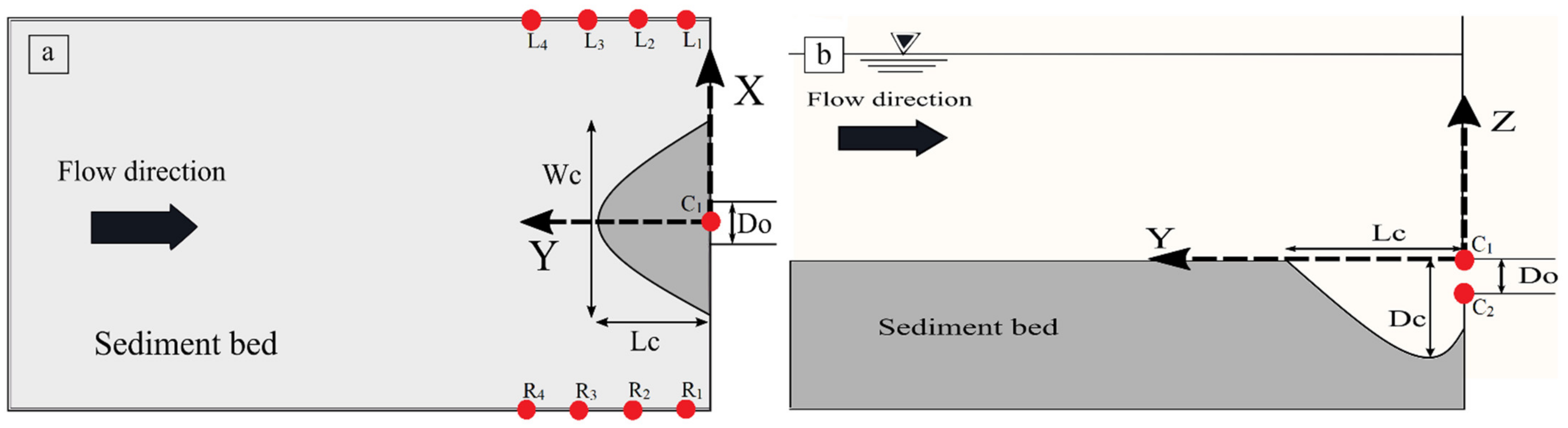
2.5.5. Surveying of Sediment Flushing Cone Geometry (SFCG)

To obtain the SFCG topography in each experiment, the SFM technique was used. After the end of each test and to ensure full drainage of the main reservoir, photographs were recorded from different positions with enough overlap on the camera rails using an advanced Canon IXUS 190 (Canon Inc., Tokyo, Japan) with a 24-megapixel resolution rate and remote-control ability. Then, the photos were analyzed in AgiSoft Metashape software (Version 1.8, Agisoft LLC, St. Petersburg, Russia) and the output of XYZ points was imported into ArcGIS as a dense-point cloud to measure the volume.

3. Results

3.1. Cube Box Test

A cube with known dimensions and volume was used to test the accuracy of the SFM tool. Therefore, the cube box was located in the reservoir, overlapping to the sediment surface level, similar to a flushed cone. To obtain the cube box topography, photographs were recorded and analyzed with SFM technique. According to the measuring distance, the typical data accuracy was determined to be 1.4 mm at 40 cm. The final data accuracy results were compared with the data accuracy results for a DPI-8 handheld scanner in Dreyer (2018) [10], and they are listed in Table 3.

3.2. Data Acquisition and Georeferencing

Before performing each test, sediment was poured layer by layer, and the surface of the sediment was levelled using a prismatic straightener according to the rulers installed in the reservoir. The first set of images was captured for the initial bed before turning on the pump. The next set of images was captured after completing each test and ensuring complete drainage of the main reservoir. Images were captured with enough overlap (70% average), and 10 MCPs in the model cover the overall area of interest.

3.3. Processing and Post-Processing

In the first step, the images were loaded into the SFM software AgiSoft Metashape, which created photos alignment and performed bundle adjustment. The next step was dense cloud generation, and then unnecessary noise was removed by trimming the dense cloud. The final step was updating the model and converting it into an absolute scale with MCPs and then replacing them with respective places. Figure 3 illustrates a 3D dense point cloud of the sediment flushing cone compared with the actual photo. In the following steps, we built the mesh, texture, tiled model, and DEM, which led to the reconstruction of the 3D model of the sediment flushing cone. Finally, the georeferenced 3D model could be extracted from the software (Figure 4).
To integrate the 3D models of sediment flushing cones with map creation tools (e.g., context labels, descriptions, interpretations, and artefacts), an Arc Map environment was used. Figure 4 illustrates the sediment flushing cone as part of the bed surface near the bottom outlet. The dense cloud produced using high-accuracy alignment contained 55,358,531 points and the polygon mesh with ultra-high quality and smooth geometry contained 17,524,712 faces. A georeferenced 3D model allows for accurate metric information and the computation of orthophotos and digital surface models (DSMs) (Figure 4) [35].

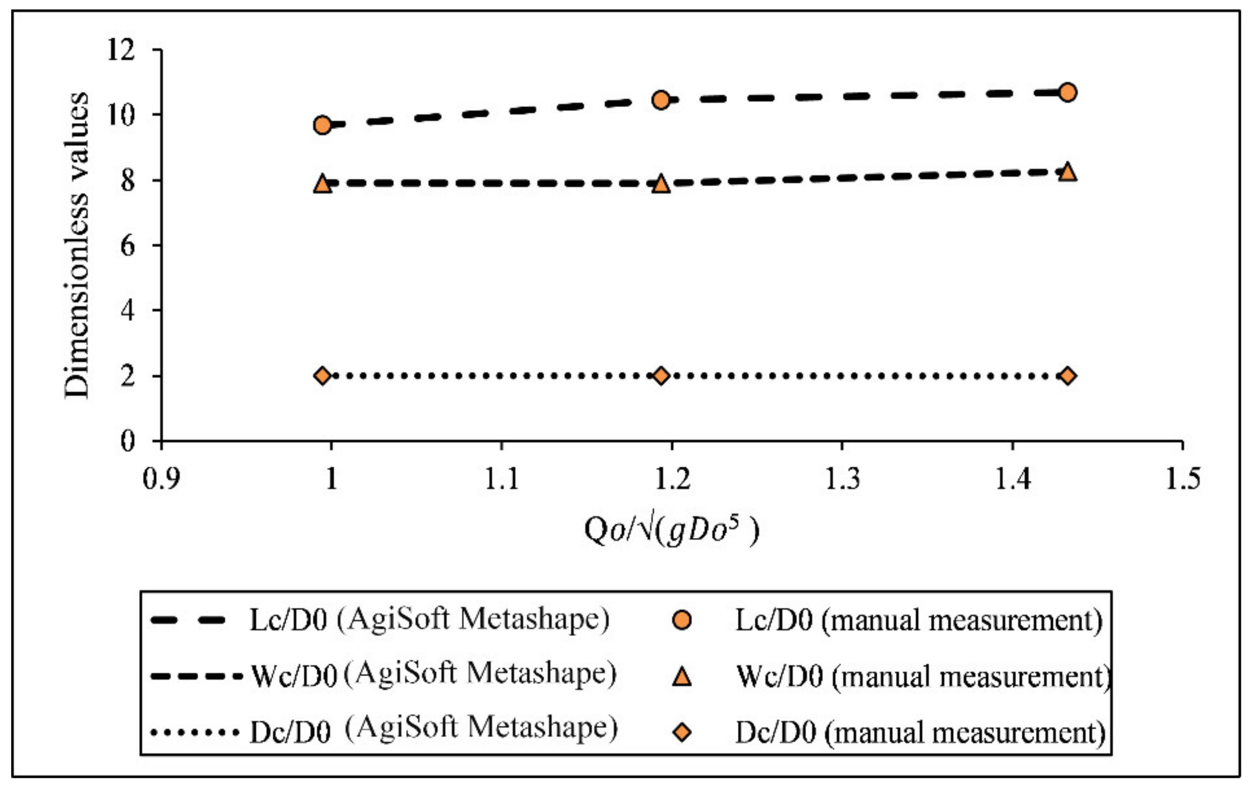
3.4. Investigation of the Surveyed Data Accuracy of Sediment Flushing Cone Dimensions with the SFM Method

After each experiment, the length, width, and depth of the sediment flushing cone (Lc, Wc, and Dc, respectively) (Figure 1) were measured manually using a laser tool. Additionally, the mentioned dimensions were measured in the AgiSoft Metashape workspace. To evaluate the data accuracy of the SFM method with the AgiSoft Metashape software, the sediment flushing cone dimensions with the best DBE structure in a full-obstruction situation (sedimentary dimensionless index of Hs/Do = 4.59) with a DBE structure with an angle of 30° between the branches, with three flow dimensionless indices of Q o g D o 5 = 0.99 , Q o g D o 5 = 1.19 , and Q o g D o 5 = 1.43 , were compared with the measured data (Figure 5). The results indicated that there was suitable agreement between the measured and calculated data.

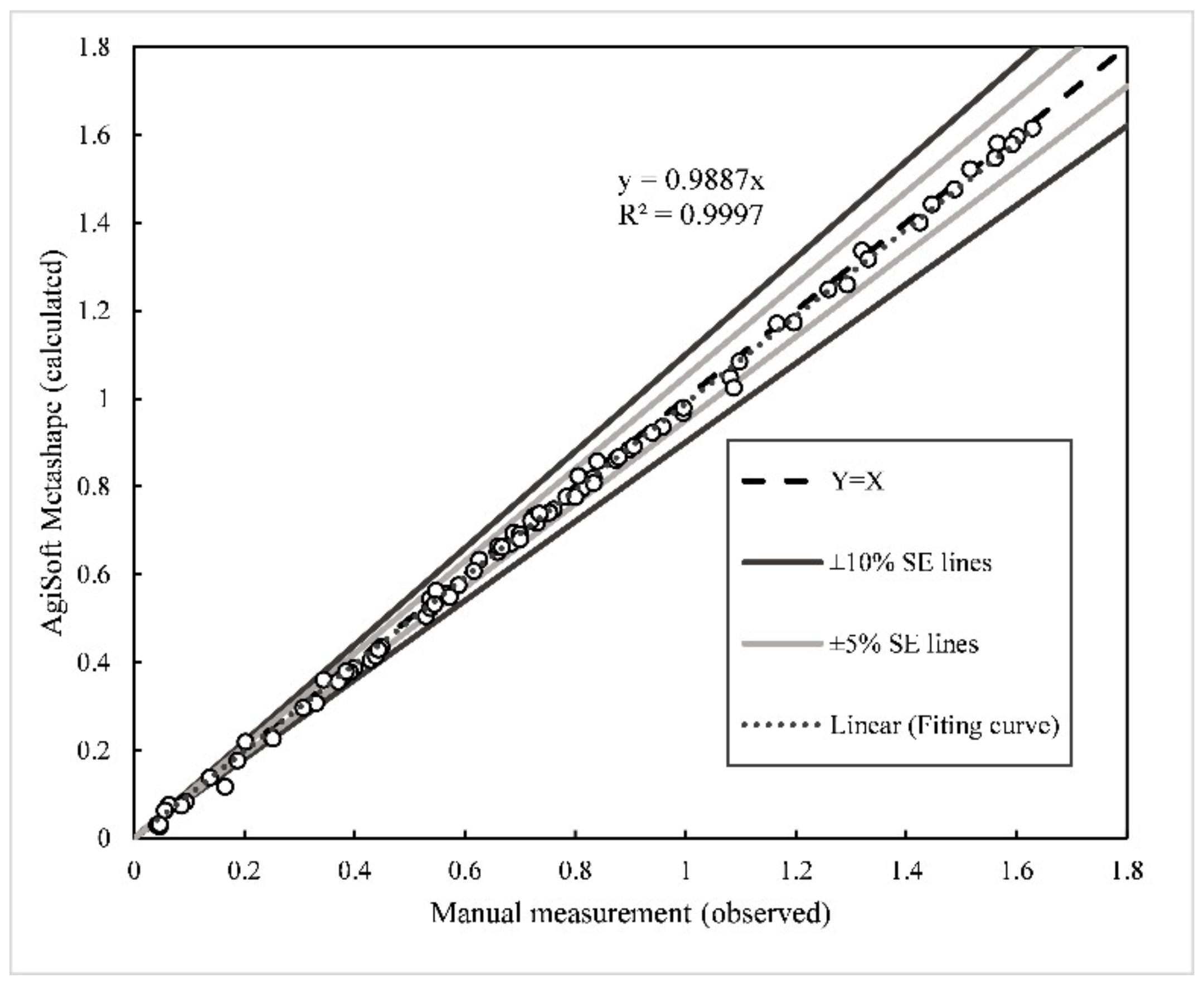
3.5. Investigation of the Surveyed Data Accuracy of Sediment Flushing Cone Cross-Section with the SFM Method

To evaluate the data accuracy of the SFM method with AgiSoft Metashape, four cross-sections were marked in various sections of the contour map generated by Surfer (Version 21, Golden Software LLC, Golden, CO, USA) (Figure 6) according to the coordinate system of the experimental setup (Figure 1). Additionally, the cross-sections were surveyed manually using a laser and mesh grid. Output data from AgiSoft Metashape were compared with the measured data at each cross-section according to the cross-section plane, as shown in Figure 7.
The data accuracy was further assessed based on a statistical analysis of the observed and calculated values of elevation dense point clouds in various coordinate systems of (x,y). Figure 8 shows the observed dimensionless values for the best operation of DBE structure in a full-obstruction situation (sedimentary dimensionless index of Hs/Do = 4.59) with a DBE structure with an angle of 30° between the branches, with flow dimensionless index of Q o g D o 5 = 1.43 of the manually measured elevation data against the values calculated using AgiSoft Metashape. According to the results and the standard error (SE) lines representing the average distance, the observed values fall from the regression line. The regression line fell between the ±5% SE lines, indicating suitable agreement between the output from the SFM software AgiSoft Metashape and the output manual measurement.

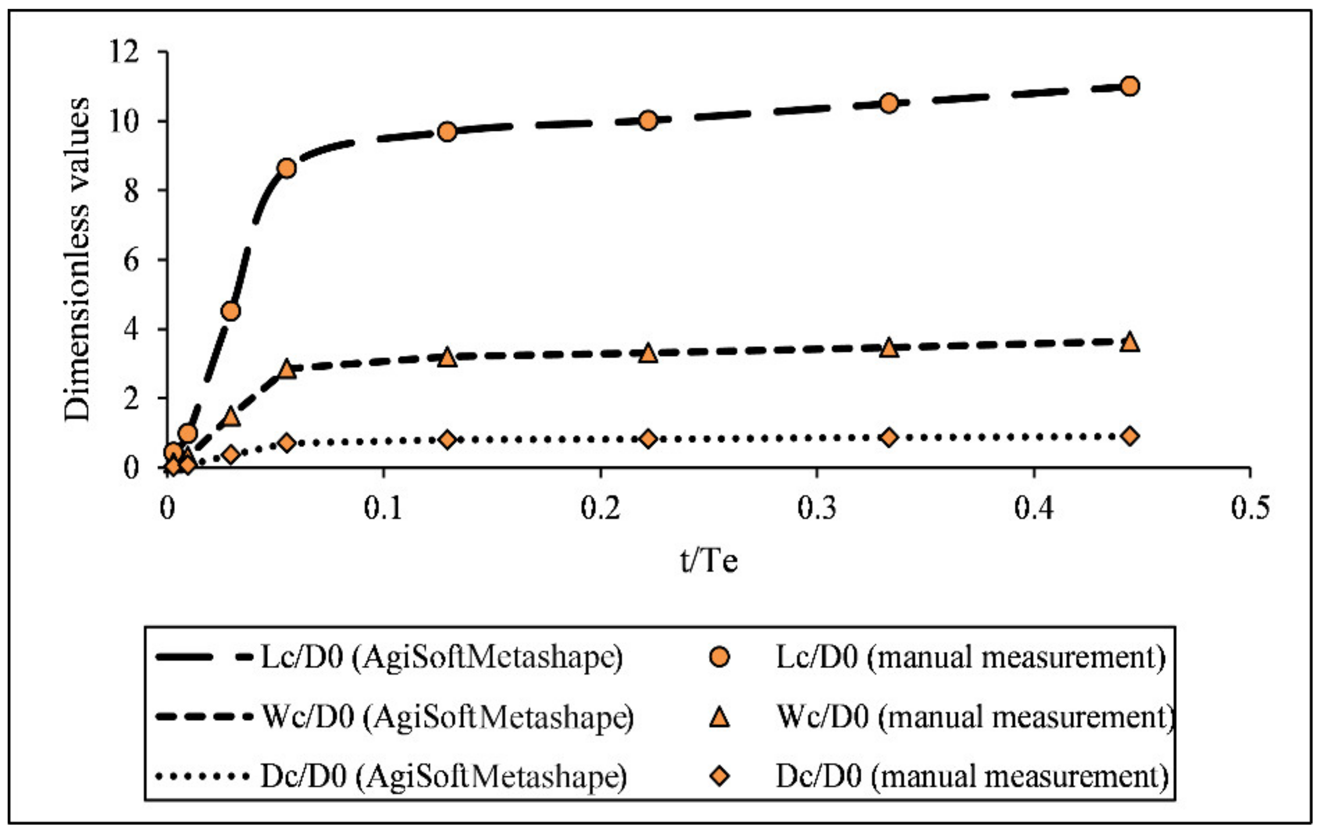
3.6. Investigation of the Accuracy of the Surveyed Data for the Temporal Development of the Sediment Flushing Cone with the SFM Method

The tests were continued until the variations in the dimensions of the sediment flushing cone were insignificant. The sediment cone starts to develop immediately after opening the low-level outlet valve when a high turbulent flow is created. In the present study, this process decreased over time, and approximately 90% of the scouring process occurred in the first 15–20 min after the start of each experiment [37]. The time duration of scouring equilibrium was 270 min, although at approximately 120 min after the beginning of each experiment, the variation in the scouring process decreased, and approximately 98% of the variation rate of sediment flushing occurred in this time period. A comparison of the manual measurement of the temporal development of the sediment flushing cone with the data output from the SFM method using the best DBE structure in a non-obstruction situation (dimensionless indices of L D B E D o = 10 , D D B E D o = 1.14 , and Q o g D o 5 = 1.43 ) is illustrated in Figure 9. The results indicated suitable agreement between the output from the SFM software AgiSoft Metashape and the output from manual measurements.

4. Discussion

4.1. Evaluation of the SFM Method Performance

SFCG data can be collected from an experimental study based on a physical model using several methods. One of the advanced methods is the use of 3D scanner tools, which has the advantage of high-quality results in a shorter time and the disadvantage of being expensive. The other methods are manual methods based on laser or point gauge and mesh grid tools, which are simple and cost-effective methods that provide low-quality results and allow for abundant time for data processing. The SFM method is a new technique based on image processing that includes short-range photogrammetry.
The results indicated that for each of the accumulation models, a regular digital camera with the default setting can be used to obtain a high level of detail for all of the point models. The validation results of the SFM method for estimating the different shapes of SFCG indicate that the results of the SFM method presented small differences with that of the manual measurements. In this method, the maximum error value was 0.512%. It should be noted that the number of photos was approximately constant, although the total number of model points relates directly to the photos used for model generation, which is consistent with the other model-based SFM photogrammetry [11,31].

4.2. Evaluation of the Data Accuracy of the Current SFM Method

To evaluate the data accuracy of the current SFM method, the dimensions, cross-sections, and temporal development of the sediment flushing cone were investigated. The results of the comparison between the observed and calculated dimensions indicated that the average error was between 0.03 mm and 0.74 mm, which illustrated a 0.26% typical accuracy. The data accuracy was further investigated by statistically analyzing the observed and calculated values of elevation dense point clouds in four cross-sections. The results indicated that the coefficient of determination for the prediction equations (R2) was 0.9997, which indicated that suitable agreement occurred between the output of the SFM software AgiSoft Metashape and the output from manual measurements. Additionally, a comparison of the data on the temporal development of the sediment flushing cone between the manual measurement and the SFM with the best DBE structure in a non-obstruction situation illustrated suitable agreement.

4.3. Data Accuracy of the Current SFM Method Compared with Other SFM Methods

In this section, the data accuracy of DEMs created by the SFM method in two hydraulic model studies was compared with the data accuracy of the current research. The mentioned DEMs based on the SFM method were used by Ruther (2019) [11] to study the bed evolution in a physical fluvial model at high sediment transport containing complex flushing hydraulic structures and by Zamani et al. (2019) [29] to determine the bed surface particle sizes, and they are compared with the current study in Table 4. Table 4 consists of the error rate between the output data from AgiSoft Metashape compared with the manually measured data and the coefficient of determination for the prediction equations (R2) for any SFM model.
The results indicated that the DEMs created by the SFM method in the two mentioned studies were consistent with the model used in the current research (Table 3). Second, the statistical parameter R2 was higher in the current research.

5. Conclusions

Certain sediment flushing cone topographic survey methods have high time consumption and produce low-accuracy output data and others have high logistical costs and require specialized user expertise; thus, a proper method that can generate accurate output data in a short period with low logistical costs is required. The current research indicates that the novel proposed technique is a cost-effective approach that provides an enhanced 3D model of the sediment flushing cone. The close-range photogrammetry method structure from motion (SFM) has been investigated for topographic surveying of sediment flushing cones. In the first step, the digital elevation model (DEM) of a cube box was determined using the SFM software AgiSoft Metashape, and its final data accuracy was compared with that obtained with a handheld scanner. In the next step, the DEM model was derived by the mentioned method for a sediment flushing cone with irregular geometric shapes, and the results were compared with manual measurements at four cross-sections surveyed performed using a laser tool. Additionally, the dimensions and temporal development of the sediment flushing cone were investigated to evaluate the data accuracy of the current SFM method. In this context, accuracy evaluation of other SFM software in comparison with AgiSoft Metashape can be considered for future development of the current study. Finally, a comparison of the observed and calculated values of the elevation dense point cloud dimensionless index, which presented an R2 value of 0.99, indicated that the SFM software AgiSoft Metashape is an accurate, cost-effective, rapid, and relatively simple method for topographic surveying of SFCG in laboratory studies.

Author Contributions

H.H. developed the methodology, performed the experimental tests and software analysis, analyzed data, and wrote the manuscript. S.A.K. provided research direction and revised the manuscript. S.B. performed some software analysis and contributed to preparation of the manuscript. M.R. and K.Q. provided their theorical and practical insights to preparation of the manuscript. All authors have read and agreed to the published version of the manuscript.

Funding

This work was supported by JSPS KAKENHI Grant Number JP21H01434.

Institutional Review Board Statement

Not applicable.

Informed Consent Statement

Not applicable.

Data Availability Statement

Not applicable.

Acknowledgments

This work was supported by JSPS KAKENHI Grant Number JP21H01434 and APN ‘Asia-Pacific Network for Global Change Research’ under project reference number CRRP2020-09MYKantoush (Funder ID: https://doi.org/10.13039/100005536).

Conflicts of Interest

The authors declare no conflict of interest.

Notations

BABundle adjustment
DCDepth of the sediment flushing cone (m)
DoDiameter of the bottom outlet (m)
DBEDendritic bottomless extended structure
DDBEDiameter of the DBE structure (m)
DEMDigital elevation model
GCPsGround control points
GISGeographic information system
L C Length of the sediment flushing cone (m)
L D B E Length of the branches of the DBE structure (m)
MCPsModel control points
Q o Outlet discharge (m3/s)
R 2 Coefficient of determination of the prediction equations
RMSERoot mean square error
S E Standard error lines representing the average distance the observed values fall from the regression line
SFMStructure from motion
SFCGSediment flushing cone geometry
SIFTScale-invariant feature transform
TTime elapsed since the beginning of the experiment (min)
T e Time duration of scour equilibrium (min)
TINTriangular irregular network
W C Width of the sediment flushing cone (m)

References

  1. Esmaeili, T.; Sumi, T.; Kantoush, S.A.; Kubota, Y.; Haun, S.; Rüther, N. Numerical Study of Discharge Adjustment Effects on Reservoir Morphodynamics and Flushing Efficiency: An Outlook for the Unazuki Reservoir, Japan. Water 2021, 13, 1624. [Google Scholar] [CrossRef]
  2. Haghjouei, H.; Rahimpour, M.; Qaderia, K.; Kantoush, S.A. Experimental study on the effect of bottomless structure in front of a bottom outlet on a sediment flushing cone. Int. J. Sediment Res. 2021, 36, 335–347. [Google Scholar] [CrossRef]
  3. Isaac, N.; Eldho, T.I. Sediment removal from run-of-the-river hydropower reservoirs by hydraulic flushing. Int. J. River Basin Manag. 2019, 17, 389–402. [Google Scholar] [CrossRef]
  4. Meshkati, M.E.; Dehghani, A.A.; Naser, G.; Emamgholizadeh, S.; Mosaedi, A. Evolution of developing flushing cone during the pressurized flushing in reservoir storage. World Acad. Sci. Eng. Technol. 2009, 3, 10–27. [Google Scholar] [CrossRef]
  5. Beiramipour, S.; Qaderi, K.; Rahimpour, M.; Ahmadi, M.M.; Kantoush, S.A. Effect of submerged vanes in front of a circular reservoir intake on sediment flushing cone. Water Manag. 2021, 174, 252–266. [Google Scholar] [CrossRef]
  6. Ahadpour Dodaran, A.; Park, S.K.; Mardashti, A.; Noshadi, M. Investigation of dimension changes in under pressure hydraulic sediment flushing cavity of storage dams under effect of localized vibrations in sediment layers. Ocean Syst. Eng. 2012, 2, 71–81. [Google Scholar] [CrossRef] [Green Version]
  7. Shahirnia, M.; Ayyoubzadeh, S.; Mohamad Vali Samani, J. Investigation on the effect of sediment level on pressurized flushing performance from reservoirs using physical model. J. Hydrol. 2014, 9, 11–25. (In Persian) [Google Scholar]
  8. Emamgholizadeh, S.; Fathi-Moghadam, M. Pressure flushing of cohesive sediment in large dam reservoirs. J. Hydraul. Eng. 2014, 19, 674–681. [Google Scholar] [CrossRef]
  9. Madadi, M.R.; Rahimpour, M.; Qaderi, K. Improving the pressurized flushing efficiency in reservoirs: An experimental study. Water Resour. Manag. 2017, 31, 4633–4647. [Google Scholar] [CrossRef]
  10. Dreyer, S. Investigating the Influence of Low-Level Outlet Shape on the Scour Cone Formed during Pressure Flushing of Sediments in Hydropower Plant Reservoirs. Master’s Thesis, University of Stellenbosch, Stellenbosch, South Africa, 2018. [Google Scholar]
  11. Ruther, N. Structure from Motion Applied to Movable Bed Scale Models. Master’s Thesis, Norwegian University of Science and Technology, Trondheim, Norway, 2019. [Google Scholar]
  12. Fonstad, M.A.; Dietrich, J.T.; Courville, B.C.; Jensen, J.L.; Carbonneau, P.E. Topographic structure from motion: A new development in photogrammetric measurement. Earth Surf. Process. Landf. 2013, 38, 421–430. [Google Scholar] [CrossRef] [Green Version]
  13. James, M.R.; Robson, S. Straightforward reconstruction of 3D surfaces and topography with a camera: Accuracy and geoscience application. J. Geophys. Res. Earth Surf. 2012, 117, F03017. [Google Scholar] [CrossRef] [Green Version]
  14. Micheletti, N.; Chandler, J.H.; Lane, S.N. Geomorphological Techniques. In Structure from Motion (SFM) Photogrammetry; Online Edition; British Society for Geomorphology: London, UK, 2014; Chapter 2, Section 2.2; ISSN 2047-0371. [Google Scholar]
  15. Westoby, M.J.; Brasington, J.; Glasser, N.F.; Hambrey, M.J.; Reynolds, J.M. ‘Structure-from-Motion’ photogrammetry: A low-cost, effective tool for geoscience applications. Geomorphology 2012, 179, 300–314. [Google Scholar] [CrossRef] [Green Version]
  16. Nyimbili, P.H.; Demirel, H.; Seker, D.Z.; Erden, T. Structure from Motion (SfM)—Approaches and Applications. In Proceedings of the International Scientific Conference on Applied Sciences, Antalya, Turkey, 27–30 September 2016. [Google Scholar]
  17. Javernick, L.; Brasington, J.; Caruso, B.S. Modeling the topography of shallow braided rivers using Structure-from-Motion photogrammetry. Geomorphology 2014, 213, 166–182. [Google Scholar] [CrossRef]
  18. Ullman, S. The Interpretation of Structure from Motion. Proc. R. Lond. Soc. B 1979, 203, 405–426. [Google Scholar]
  19. Holata, L.; Plzák, J.; Světlík, R.; Fonte, J. Integration of Low-Resolution ALS and Ground-Based SfM Photogrammetry Data. A Cost-Effective Approach Providing an ‘Enhanced 3D Model’ of the Hound Tor Archaeological Landscapes (Dartmoor, South-West England). Remote Sens. 2018, 10, 1357. [Google Scholar] [CrossRef] [Green Version]
  20. Bomminayun, S.; Stoesser, T. Turbulence Statistics in an Open-Channel Flow over a Rough Bed. J. Hydraul. Eng. 2011, 137, 1347–1358. [Google Scholar] [CrossRef]
  21. Dietrich, J.T. Applications of Structure-from-Motion Photogrammetry to Fluvial Geomorphology. Ph.D. Thesis, University of Oregon, Eugene, OR, USA, 2014. [Google Scholar]
  22. Smith, M.W.; Carrivick, J.L.; Hooke, J.; Kirkby, M.J. Reconstructing flash flood magnitudes using “Structure-from-Motion”: A rapid assessment tool. J. Hydrol. 2014, 519, 1914–1927. [Google Scholar] [CrossRef]
  23. Kasprak, A.; Wheaton, J.; Ashmore, P.; Hensleigh, J.; Peirce, S. The relationship between particle travel distance and channel morphology: Results from physical models of braided rivers. J. Geophys. Res. Earth Surf. 2014, 120, 55–74. [Google Scholar] [CrossRef]
  24. Thumser, P.; Kuzovlev, V.; Zhenikov, K.; Zhenikov, Y.; Boschi, M.; Boschi, P.; Schletterer, M. Using structure from motion (SFM) technique for the characterization of riverine systems—Case study in the headwaters of the Volga River. Geogr. Environ. Sustain. 2017, 10, 31–43. [Google Scholar] [CrossRef] [Green Version]
  25. Ferreira, E.; Chandler, J.; Wackrow, R.; Shiono, K. Automated extraction of free surface topography using SfM-MVS photogrammetry. Flow Meas. Instrum. 2017, 54, 243–249. [Google Scholar] [CrossRef] [Green Version]
  26. Duró, G.; Crosato, A.; Kleinhans, M.; Uijttewaal, W. Bank erosion processes measured with UAV-SfM along complex banklines of a straight mid-sized river reach. Earth Surf. Dyn. 2018, 6, 933–953. [Google Scholar] [CrossRef] [Green Version]
  27. Masoudi, A.; Noorzad, A.; Majdzadeh Tabatabai, M.R.; Samadi, A. Application of short-range photogrammetry for monitoring seepage erosion of riverbank by laboratory experiments. J. Hydrol. 2018, 558, 380–391. [Google Scholar] [CrossRef]
  28. Naves, J.; Anta, J.; Puertas, J.; Regueiro-Picallo, M.; Suárez, J. Using a 2D shallow water model to assess Large-scale Particle Image Velocimetry (LSPIV) and Structure from Motion (SfM) techniques in a street-scale urban drainage physical model. J. Hydrol. 2019, 575, 54–65. [Google Scholar] [CrossRef]
  29. Zamani, P.; Mohajeri, H.; Samadi, A. Application of Structure from Motion (SFM) Method to Determine the Bed Surface Particles Sizes in Gravel Bed Rivers. Iran J. Soil Water Res. 2019, 50, 215–230. [Google Scholar] [CrossRef]
  30. Šiljeg, A.; Marić, I.; Cukrov, N.; Domazetović, F.; Roland, V. A Multiscale Framework for Sustainable Management of Tufa-Forming Watercourses: A Case Study of National Park “Krka”, Croatia. Water 2020, 12, 3096. [Google Scholar] [CrossRef]
  31. Spreitzer, G.; Tunnicliffe, J.; Freidrich, H. Large wood (LW) 3D accumulation mapping and assessment using structure from Motion photogrammetry in the laboratory. J. Hydrol. 2020, 581, 124430. [Google Scholar] [CrossRef]
  32. Snavely, N.; Seitz, S.M.; Szeliski, R. Modeling the World from Internet Photo Collections. Int. J. Comput. Vis. 2008, 80, 189–210. [Google Scholar] [CrossRef] [Green Version]
  33. Furukawa, Y.; Ponce, J. Accurate, dense, and robust multi-view stereopsis. In Proceedings of the IEEE Conference on Computer Vision and Pattern Recognition (CVPR), Minneapolis, MN, USA, 17–22 June 2007. [Google Scholar]
  34. Agisoft Metashape Version 1.8: User Manual: Professional Edition. 2022. Available online: https://www.agisoft.com/pdf/metashape-pro_1_8_en.pdf (accessed on 12 March 2022).
  35. De Reu, J.; De Smedt, P.; Herremans, D.; Van Meirvenne, M.; Laloo, P.; De Clercq, W. On introducing an image-based 3D reconstruction method in archaeological excavation practice. J. Archaeol. Sci. 2014, 41, 251–262. [Google Scholar] [CrossRef]
  36. Beiramipour, S.; Qaderi, K.; Rahimpour, M.; Ahmadi, M.M.; Kantoush, S.A. Investigation of the Impacts of Submerged Vanes on Pressurized Flushing in Reservoirs. Iran J. Soil Water Res. 2020, 51, 2187–2201. (In Persian) [Google Scholar]
  37. Haghjouei, H.; Rahimpour, M.; Qaderia, K.; Kantoush, S.A. Experimental Investigation of Temporal Development of the Sediment Flushing Cone in Reservoirs Affected by DBE Structure. Iran J. Soil Water Res. 2020, 51, 2221–2233. (In Persian) [Google Scholar] [CrossRef]
Figure 1. Schematic representation of MCPs in the coordinate system of the experimental setup: top view (a) and side view (b) [2].
Water 14 01588 g001
Figure 2. Schematic representation of the structures used in the current research.
Water 14 01588 g002
Figure 3. Three-dimensional dense point cloud in the software workspace (left) and real image of the sediment flushing cone (right).
Water 14 01588 g003
Figure 4. Orthophoto (left) and DSM (right) of the sediment flushing cone.
Water 14 01588 g004
Figure 5. Output data from AgiSoft Metashape based on the best DBE structure in a full-obstruction situation using various indices of flow (dimensionless) compared with the manually measured data.
Water 14 01588 g005
Figure 6. Cross-section plane of the sediment flushing cone.
Water 14 01588 g006
Figure 7. Output data from AgiSoft Metashape compared with the manually measured data at cross-sections (1-1) (a), (2-2) (b), (3-3) (c), and (4-4) (d) according to the cross-section plan.
Water 14 01588 g007
Figure 8. Observed vs. calculated values of the elevation dense point cloud dimensionless index (note: SE lines are the standard error lines representing the average distance the observed values fall from the regression line, linear (fitting curve) is the regression line indicating the agreement rate between the observed and calculated values, and R2 is the coefficient of determination of the prediction equations).
Water 14 01588 g008
Figure 9. The accuracy of the temporal development of the sediment flushing cone with AgiSoft Metashape in comparison with the manually measured data using the best DBE structure in the no obstruction situation in various indices of flow dimensionless (note: t / T e is the dimensionless index of time elapsed since the beginning of the experiment, where t is the time elapsed since the beginning of the experiment (min) and T e is the time duration of scour equilibrium (min)).
Water 14 01588 g009
Table 1. Georeferencing accuracy of the model based on a comparison between the real and estimated X-, Y-, and Z-coordinate systems per MCP. The total RMSE is presented at the bottom of the table.
MCPX (m)Y (m)Z (m)EX
(m)
EY
(m)
EZ
(m)
(EX)2(EY)2(EZ)2RMSE
(m)
L11.250.1101.93 × 10−33.10 × 10−42.60 × 10−43.71 × 10−69.61 × 10−86.76 × 10−81.97 × 10−3
L21.250.3301.55 × 10−35.60 × 10−42.10 × 10−42.40 × 10−63.14 × 10−74.41 × 10−81.66 × 10−3
L31.250.5503.85 × 10−32.20 × 10−41.85 × 10−31.48 × 10−54.84 × 10−83.42 × 10−64.28 × 10−3
L41.250.7701.00 × 10−31.65 × 10−38.20 × 10−41.00 × 10−62.72 × 10−66.72 × 10−72.10 × 10−3
R1−1.250.1105.50 × 10−48.20 × 10−41.60 × 10−33.03 × 10−76.72 × 10−72.56 × 10−61.88 × 10−3
R2−1.250.3302.00 × 10−41.10 × 10−39.50 × 10−44.00 × 10−81.21 × 10−69.03 × 10−71.47 × 10−3
R3−1.250.5501.55 × 10−31.55 × 10−31.71 × 10−32.40 × 10−62.40 × 10−62.92 × 10−62.78 × 10−3
R4−1.250.7701.80 × 10−32.50 × 10−41.23 × 10−33.24 × 10−66.25 × 10−81.51 × 10−62.19 × 10−3
C10008.50 × 10−49.60 × 10−41.95 × 10−37.23 × 10−79.22 × 10−73.80 × 10−62.33 × 10−3
C200−0.115.50 × 10−41.65 × 10−38.58 × 10−43.03 × 10−72.72 × 10−67.36 × 10−71.94 × 10−3
2.26 × 10⁻³
Table 2. Experimental setup in the current research [2].
Test No.NameQo
(L/s)
Hs
(cm)
Test No.NameQo
(L/s)
Hs
(cm)
Test No.NameQo
(L/s)
Hs
(cm)
1a1,112.539.516a1,212.54531a1,312.550.5
2b1,117b1,232b1,3
3c1,118c1,233c1,3
4d1,119d1,234d1,3
5e1,120e1,235e1,3
6a2,11521a2,21536a2,315
7b2,122b2,237b2,3
8c2,123c2,238c2,3
9d2,124d2,239d2,3
10e2,125e2,240e2,3
11a3,11826a3,21841a3,318
12b3,127b3,242b3,3
13c3,128c3,243c3,3
14d3,129d3,244d3,3
15e3,130e3,245e3,3
Note: xi,j, where x = structure type, which consists of a, b, c, d, and e, with a = DBE 30°, b = DBE 45°, c = DBE 60°, d = PSC structure, and e = reference test (no-structure); and i,j = indices of discharge and sediment height, with i = 1, 2, and 3 representing discharges of 12.5, 15, and 18 L/s, respectively, and j = 1, 2, and 3 representing sediment heights of 39.5, 45, and 50.5 cm, respectively.
Table 3. Data accuracy results of the SFM and comparison with the accuracy of a DPI-8 handheld scanner.
Range (m)DPI-8 Handheld ScannerSFM
Typical Accuracy (RMSE)Minimum AccuracyTypical Accuracy (RMSE)Minimum Accuracy
<10.20%0.5%0.26%0.51%
1–20.50%0.8%0.31%0.58%
Table 4. Data accuracy comparison between the different SFM models.
SFM ModelPurposeError Rate
(mm)
R2 (Dimensionless)
Ruther (2019) [11]Determining the bed in a physical fluvial model0.05–2.960.9965
Zamani et al. (2019) [29]Determining the bed surface particles sizes0.67–1.10.98
The current studyDetermining the sediment flushing cone dimensions0.03–0.740.9997
Publisher’s Note: MDPI stays neutral with regard to jurisdictional claims in published maps and institutional affiliations.

