Estimating Point and Nonpoint Source Pollutant Flux by Integrating Various Models, a Case Study of the Lake Hawassa Watershed in Ethiopia’s Rift Valley Basin

Abstract

Increasing pollutant emissions in the Lake Hawassa watershed (LHW) has led to a severe water quality deterioration. Allocation and quantification of responsible pollutant fluxes are suffering from scarce data. In this study, a combination of various models with monitoring data has been applied to determine the fluxes for Chemical Oxygen Demand (COD), Biochemical Oxygen Demand (BOD₅), Total Dissolved Solid (TDS), Total Nitrogen (TN), Nitrate and Nitrite-nitrogen (NOx-N), Total Phosphorous (TP) and phosphate (PO₄-P). Water, wastewater and stormwater samples were collected and analyzed at eight monitoring stations from rivers and point sources and six monitoring stations of stormwater samples. The flow simulated with soil and water assessment tool (SWAT) could be very well calibrated and validated with gauge data. This flow from SWAT model, measured flow during monitoring and pollutant concentrations were used in FLUX32 to estimate pollutant fluxes of main rivers and point sources in LHW. The formulas provided by Ethiopian Roads Authority and Gumbel’s theory of rainfall frequency analysis was employed to determine the 2-years return period rainfall depth for the City of Hawassa. The integration of HEC-GeoHMS and SCS-CN with the catchment area enabled to determine stormwater pollution load of Hawassa City. The estimated pollutant flux at each monitoring stations showed that the pollutant contribution from the point and nonpoint sources prevailing in the study area, where the maximum fluxes were observed at Tikur-Wuha sub-catchments. This station was located downstream of the two point sources and received flow from the upper streams where agricultural use is predominant. Furthermore, Hawassa city has been identified as a key pollutant load driver, owing to increased impacts from clearly identified point sources and stormwater pollutant flux from major outfalls. Agricultural activities, on the other hand, covers a large portion of the catchment and contributes significant amount to the overall load that reaches the lake. Thus, mitigation measures that are focused on pollutant flux reduction to the lake Hawassa have to target on the urban and agricultural activities.

1. Introduction

Currently due to the rapid advances in modelling, numerous water quality models were developed with various modelling algorithms for various land use and water bodies for pollutants at different spatio-temporal scales [1,2]. The data demand for water quality models increase with the complexity and scope of application [3].

Generally, most developed countries, namely the US or European countries have established better and advanced surface water quality models [2]. One of pivotal factors in the primary goals of environmental management would be assessing the water quality despite limited observations [4]. In the developing world reliable application of water quality models is often challenging owing to lack of sufficient and quality data and access to patented software is limited by finances. Furthermore, nearly for all rivers the gauged data are limited and fragmented. The Rift Valley Lake basin is among the data scarce areas of Ethiopia and the historical measured pollutant flux including sediment data is very limited [5,6]. In Hawassa, on the other hand, wastewater management is a big concern because most residents use latrines. Wastewater treatment plants for the partly existing sewer system for buildings with flushing systems is missing [7] and stormwater is discharged without any treatment. Furthermore, Lake Hawassa is encircled by agricultural land, residential places, industrial and commercial hubs and is located near the city of Hawassa. As a result, it is prone to a range of environmental risks and the water quality deteriorates over time, posing a danger to the biodiversity [8]. Hence, studying the pollutant load of the basin is necessary to obtain more realistic information [5].

The estimation of pollutants load from non-point sources is usually accomplished by means of watershed models. However, due to the intensive input data requirements and complexity by most of the models, it is disconcerting to quantify diffuse source loads in developing countries such as Ethiopia owing to limited hydrological, meteorological and water quality data [9,10].

In order to fulfil the existing gaps in the developing world such as Ethiopia, setting up frequent monitoring and assessment is a critical task. In this sense, simple models that do not require intensive input datasets are worthwhile common approaches for the prediction of diffuse pollutions from various land uses including urban and industrial land uses [11,12,13].

On such occasion, a common approach such as pollutant export coefficients representing the rate of pollutant loadings by land area, that predict an annual load from land to water, are often a discretionary means to estimate loadings from non-point sources [6,14,15]. Export coefficients modelling is a simple approach that can be adopted for data-poor areas and for preliminary assessments connecting land use to water quality. It is generally based on the postulation that a particular land use will export distinctive magnitudes of pollutants to a downstream water body on a yearly basis [16]. To justify this postulation, the pollutant export coefficients must be developed for the locally specific conditions [15]. If this is achieved, reliable and relatively accurate pollutant transport models can be set up to support watershed level point and nonpoint source pollution management [17].

Therefore, in this study we employed pollutant loading estimator (PLOAD) to determine the pollution loads with the help of export coefficient modelling. The approach was used as a means of preliminary pollutant load estimation at different watersheds in Ethiopia [6,9], Tanzania [18], China [10,19], USA [20], Japan [15], UK [12], Lithuania [21], Egypt [22], Philippines [23] and Rwanda [24].

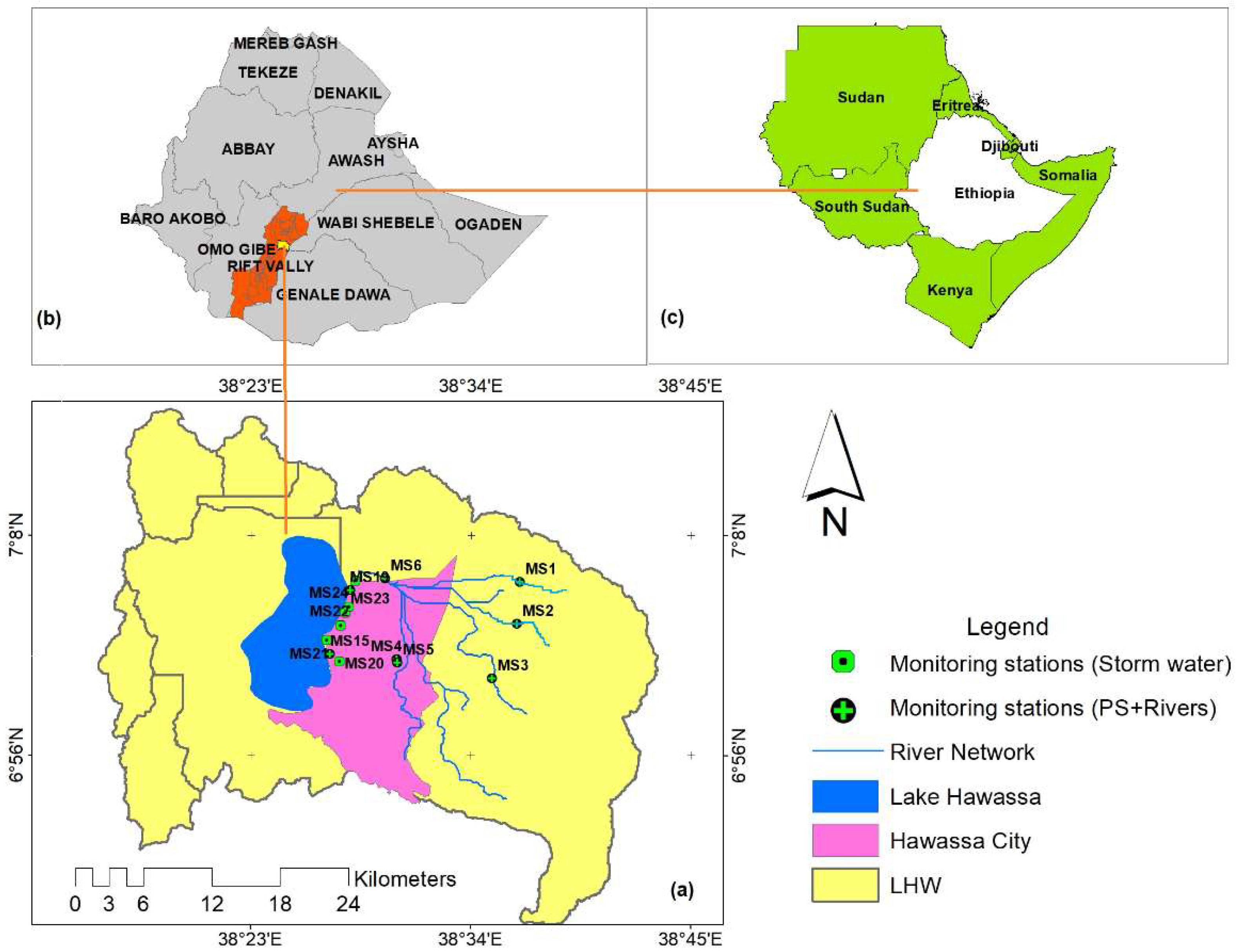
The watershed of lake Hawassa comprises rural and urban areas. So, for conducting a comprehensive pollutant flux in the watershed, pollutant flux of (i) rivers, (ii) point sources (PS) and (iii) urban stormwater runoff have to be investigated. Namely the impact of stormwater runoff has so far not been addressed and requires a deeper investigation. A prerequisite for this is a reliable runoff information at watershed scale. In recent decades a number of hydrological models have been developed and used to envisage the runoff information in different hydrological units over years. A widely used approach to estimate runoff from spatial data is the Soil Conservation Service curve number (SCS-CN) method [25,26]. In this study, we also applied the SCS-CN method to estimate rainfall-runoff depth for the city of Hawassa.

A characteristic problem in the watershed under investigation is the lack of sufficient monitoring water quality data due to budget constraint. This complicates prediction of pollutant loads from point and non-point sources, as land use, emissions and ambient water quality cannot be linked directly. Currently the government focuses on the reduction in the point source pollution. However, estimation of pollutant flux from nonpoint sources in data-limited watersheds in Ethiopia (in general and in the study area in particular) are perplexing, due to lack of baseline data to direct development targets. Thus, the use and identification of simple, cost effective and economical water quality models is greatly imperative to estimate the pollutant flux of rivers and point sources that are in turn helpful for surface water quality management. To support this target, this study is aimed at determining the annual pollutant loads contributions from point, nonpoint sources and stormwater to the Lake Hawassa watershed, identify the probable pollution flux hotspots and calibration of pollutant export coefficient for the study area by integrating PLOAD, SWAT, FLUX32, HEC-GeoHMS and SCS-CN with monitoring data.

2. Materials and Methods

2.1. Study Area

Ethiopia has endowed with several lakes of volcanic and tectonic origins, among which Lake Hawassa is an endorheic freshwater lake formed in collapsed calderas and located in Lake Hawassa Watershed (LHW) [27]. Within the Central Ethiopian Rift Valley Basin, the Lake watershed is located between 6°45′ and 7°15′ N latitude and 38°15′ to 38°45′ E longitude, in Sidama and Oromiya Regional States (Figure 1), covering 1431 km² [28].

Streams from the eastern catchment flow to Lake Cheleleka wetland and are drained by the Tikur-Wuha River that feeds Lake Hawassa. Tikur-Wuha River is the main rivers in Lake Hawassa watershed, located in the middle section of the catchment where most of the untreated household and industrial wastewater are discharged. The Lake has been used as the main source for drinking, irrigation, aquatic life and recreational uses. Despite this, the lake and its tributaries has been affected by various sources of pollution [7].

The climate of the Hawassa sub-basin is sub-humid and distinctly seasonal. The months from April to October are wet and humid, and the main rainy season is between July and September, the area receives a mean precipitation of 1028 mm rainfall annually. The mean minimum precipitation is 17.8 mm in December (dry season) and the mean maximum precipitation is 119.8 mm in August (rainy season) [29]. The long term mean annual temperature of the area varies from 12.5 to 26 °C [30], whereas the mean monthly evapotranspiration in the low lands ranges from 39 mm in July to 100 mm in January [29].

2.2. Sampling and Analysis of Monitoring Parameters

Water, wastewater and stormwater sample were collected and analyzed for some selected physicochemical parameters in the Lake Hawassa watershed from March 2020 to December 2020. Sample collection for the wet season were conducted after rainfall events. The locations of monitoring stations were determined using Global navigation satellite system. Water temperature, pH, total dissolved solids and conductivity were determined onsite. For the estimation of pollutant flux in the Lake Hawassa watershed, water and wastewater samples were collected from eight monitoring stations from rivers and point sources (Figure 1,

Table 1. Monitoring stations from rivers in Lake Hawassa Watershed.

Code	Monitoring Sites	Latitude (Y)	Longitude (X)	Area (ha)
MS1	Wesha River	7°5′13.8″	38°36′51.3″	5754.9
MS2	Hallo River	7°3′14.4″	38°36′43.2″	4152.3
MS3	Wedessa River	7°0′21.6″	38°35′6.0″	14,615.5
MS6	Tikur-Wuha River	7°5′22.6″	38°30′25.4″	61,479.8

and

Table 2. Monitoring stations from point sources in Lake Hawassa Watershed.

Code	Monitoring Sites	Latitude (Y)	Longitude (X)	Altitude (Z)
MS4	BGI effluent discharge site	7°1′31.8″	38°30’57.4″	1686
MS5	Moha Soft Drinks Factory	7°1′26.9″	38°30’47.5″	1671
MS15	Referral Hospital	7°1′47.6″	38°27’46.1″	1686
MS19	Hawassa Industrial Park	7°4′49.4″	38°28’44.4″	1690

). Monitoring stations for stormwater in Hawassa City were established at the major outlets to monitor the urban stormwater quality. The urban runoff samples were collected from six monitoring stations for two rainfall events (Figure 1 and

Table 3. Monitoring stations for stormwater from outfalls of drainage system in Hawassa City.

Code	Monitoring Sites	Latitude (Y)	Longitude (X)	Area (ha)
MS20	Near Referral Hospital	7°1′28.71″	38°28′14.63″	306
MS21	Near Amora-Gedel	7°2′30.67″	38°27′37.83″	206.6
MS22	Near Fiker Hayk	7°3′12.99″	38°28′18.46″	97
MS23	Near Chambalala Hotel	7°3′48.37″	38°28′31.07″	377.4
MS24	Near ELPA office	7°4′4.86″	38°28′41.68″	95
MS25	Near South spring Hotel	7°5′29.34″	38°28′56.12″	123.6

).

Composite samples were collected in pre-cleaned 2 L polyethylene plastic bottles that are sterilized for biochemical oxygen demand (BOD) and chemical oxygen demand (COD) analyses. The bottles were washed with concentrated nitric acid and distilled water before sample collection and placed in a cooler box, kept under 4 °C and immediately transported to the laboratory for analysis. Samples of nitrate and phosphate were prefiltered at site and kept in a cooler box before analysis. The analytical methods and instruments used for analysis are shown in

Table 4. Analytical methods and instruments used for the analysis of selected parameters in LHW.

Parameters	Analytical Methods and Instruments
TDS	Portable multi-parameter analyzer, Zoto, Germany
BOD5	Manometric, BOD sensor
COD	Closed Reflux, Colorimetric
PO4-P and TP	Spectrophotometrically by molybdovandate (Hach DR-3900)
NO3-N	Photometric measurements, Wagtech Photometer 7100 at 520 nm wavelength
NO2-N	Spectrophotometrically by salicylate, (Hach DR-3900)
TN	Spectrophotometrically by persulfate digestion (Hach DR-3900)

. All the analytical methods were carried out according to the standard methods for the examination of water and wastewater [31].

2.3. Data Treatment

The data treatment needs to be performed for missing data and outliers in the climate and monitored water quality data before executing SWAT, PLOAD, FLUX32 and Gumbel’s theory of distribution. Hence, outliers were treated according to Grubbs [32] test approach with XLSTAT 2016. However, missing data was handled by the multiple imputation of missing values technique using Markov Chain Monte Carlo method [33].

2.4. Estimation of Flow

Instantaneous flow in study basin has been measured at the time of sample collection using the current meter (Toho Dentan CMS-11C, Tokyo, Japan). Since flow and pollutant concentrations are dynamic, determination of time series data of flow is crucial besides the instantaneous flow. In the study watershed under investigation, there are four monitoring stations in the study area out of which only one station is gauged and having stream flow records, the other three lack stream flow records. The problem of missing records can be circumvented by model based flow estimations [9,15]. In order to estimate the discharge at the ungauged sites, we applied the soil and water assessment tool (SWAT), a semi-distributed, process-oriented hydrological watershed-scale model [34]. The input data to the model-like land use map, digital elevation model (DEM), soil map, hydrology (stream flow) and weather data were collected from Ministry of Water, Irrigation and Electricity, Ethiopian meteorology Agency. The basic concept of the model is to subdivide a basin into sub-basins and further combine land cover, soil and slope to obtain the hydrologic response unit (HRU) where all land areas have homogeneous land use, soil and slope combinations. In each HRU, hydrological components are calculated for surface water, soil and groundwater [35]. Accordingly, the SWAT model was simulated from 1996–2015 where two-year warmup period, twelve years (1998–2009) calibration and 6 years (2010–2015) of validation for the full data available. The flow calibrated and validated by SWAT at Tikur-Wuha catchment was used to generate flow in the ungauged sub-catchment outlets (monitoring stations) in Tikur-Wuha catchment and later used as an input for FLUX32 for pollutant load estimation along with the instantaneous flow and measured pollutant concentrations.

In this juncture, the area ratio-based method was among the streamflow transfer techniques that has been used to estimate the streamflow at ungauged stations from the SWAT calibrated flow. In the area ratio technique, the single source area ratio method is widely used and the easiest approach to determine the runoff at ungauged stations [36]. The transfer of flow from the gauged to the ungauged was reasonable as the ungauged catchments are located within the gauged catchment having similar hydrological, meteorological, land use and soil properties. Hence, the streamflow at an ungauged site is estimated by using Equation (1) taken from [37].

$$\frac{{\mathrm{Q}}_{\mathrm{y}}}{{\mathrm{Q}}_{\mathrm{x}}}=\frac{{\mathrm{A}}_{\mathrm{y}}}{{\mathrm{A}}_{\mathrm{x}}}$$

(1)

where, A_x and A_y are the drainage area of the ungauged and gauged site, respectively, Q_x is the observed streamflow at a gauged site, and Q_y is the estimated discharge at an ungauged site.

2.5. Watershed Model Selection

Examination of pollutant loads from point and non-point sources that are contributing to pollution of surface water bodies are crucial for watershed management. A number of physical and empirical models has been established to comprehend complex hydrological and ecological processes associated with point and nonpoint source pollution [38].

The mechanistic watershed models can provide more accurate results on pollutant losses, but such models need a huge amount of input data. These intensive input data requirements make such a modelling a highly challenging task hindering its use [39]. Thus, for estimation of pollutant load the local conditions and data availability should be taken in to consideration for selection of models [10].

There exist various watershed and river models with different focus and abilities. Before selecting an appropriate approach, we reviewed commonly applied models with regard to our goals and data availability (

Table 5. Some selected modelling tools and their selection criteria evaluation.

Name of the Model and References	Characteristics	Application Domain of the Model	Accessibility of the Software	Input Data Requirement
AGNPS [40]	A distributed model that evaluates the agricultural NPS pollution and simulates the transport of sediments and chemicals	Catchment	Public domain	Data-intensive
GWLF [41]	A semi-distributed/lumped model that estimates runoff, sediment and nutrient loadings	Catchment	Public domain	Moderate
MONERIS [42]	A conceptual model, which allows the quantification of nutrients emissions via various point and diffuse pathways into river systems	river	Public domain	Data-intensive
MIKE 11 [43]	A distributed hydrodynamic model of flow and water quality in streams and simulates solute transport and transformation in complex river systems	River	Proprietary	Data-intensive
QUAL2E [44]	A one dimensional and steady-state model typically used for water quality modelling of pollutants in rivers, streams and well-mixed lakes	River/Lake	Public domain	Minimum
SPARROW [45]	Semi distributed statistical regression model that is designed to account for the spatial variability in contaminant flux in stream water quality to impose the mass balance	Catchment/River	Proprietary	Data-intensive
HSPF [46]	An analytical tool designed to simulate hydrology and water quality for conventional and toxic organic pollutants	Catchment/River	Public domain	Data-intensive
PLOAD in BASINS 4.5 System [47]	A Simple or an export coefficient based method that is used to estimate NPS contribution from each land use by incorporating point source and GIS-based land-use data	Catchment level	Public domain	Minimum
SWMM [48]	A distributed physically based, dynamic, continuous urban stormwater runoff quantity and quality model	Urban catchment	Public domain	Data-intensive
WASP [49]	A surface water quality modelling tool used to analyse a variety of water quality problems in water bodies such as ponds, rivers/streams, lakes/reservoirs, estuaries and coastal waters	River/Lake	Public domain	Data-intensive
SWAT [35]	A semi-distributed model that is used for the prediction of the effects of alternative land use management practice on water, sediment, crop growth, nutrient cycling, and pesticide in watersheds with varying soils, land use and management conditions	Catchment level	Public domain	Data-intensive
AGWA [50]	A distributed multipurpose hydrologic analysis system that integrated several sub-models to predict runoff and erosion rates	Catchment level	Public domain	minimum

).

Among the reviewed models BASINS (better assessment science integrating point and nonpoint sources) model is a comprehensive watershed model framework that integrates numerous watershed models such as SWAT (Soil and Water Assessment Tool, Austin, TX, USA), HSPF (Hydrological Simulation Program FORTRAN, Athens, GA, USA), GWLF-E (Generalized Watershed Loading Function, Ithaca, NY, USA), SWMM (Stormwater Management Model, Cincinnati, OH, USA), PLOAD (Pollutant Loading Estimator, Athens, GA, USA) and instream and water quality models such as AQUATOX and WASP (Water Quality Analysis Simulation Program, Athens, GA, USA) as plug-ins was found to be the most plausible option for the watershed under investigation [47].

Many researchers were in favour of PLOAD model due to its capability and adaptability in different watersheds [6,9,10]. Angello et al. [9] and Belachew et al. [6] engaged PLOAD model to estimate the point and nonpoint source pollutant loads in data-scarce Little Akaki and Borkena Rivers in Ethiopia, respectively and both suggested the use of PLOAD model in data-poor catchments for point and nonpoint source pollutant load estimation. In this study, therefore, we used the PLOAD model due to its adaptability and small number of input data requirement.

PLOAD (pollutant loading Estimator) is a BASINS plugin, developed by Cornell, Howland, Hayes, Merryfield and Hill (CH2M-HILL) is a simple model that uses GIS-based data sources such as land use, watershed shapefile, export coefficient (EC) and allows best management practices (BMP) specifications and point sources load. In PLOAD the point and non-point nutrient loads from each land use for the physicochemical parameters (BOD, COD, TN, PO₄-P, NOx-N and TDS) were estimated based on the export coefficients and can be applied for urban, suburban and rural areas [20,51,52].

PLOAD uses two approaches to estimate the point and the nonpoint sources load contribution: simple and export coefficient method. Both approaches can be applied based on data availability and applicability on a watershed. However, a simple method is used in smaller watersheds, usually, less than 1 square mile, whereas the export coefficient approach was used to compute the annual pollutant loads in a mixed land use and can be run for multiple scenarios [6,11,20,47,51,52].

In the study area, we used the export coefficient approach where pollutant loads in PLOAD are calculated by

$$\mathrm{PL}={\displaystyle {\sum }_{\mathrm{i}=1}^{\mathrm{n}}\mathrm{EC}\ast \mathrm{ALu}}$$

(2)

where PL is the pollutant loading rate for land use type (kg yr⁻¹), ALu is the area of the land use type Lu (ha). To estimate diffuse pollution, each land use category has been assigned the export coefficient values (kg ha⁻¹ yr⁻¹).

2.6. Pollutant Export Coefficient

The export coefficients (ECs) are distinct values of the specific attributes for a particular land-use and a measure of the total quantity of pollutants exported from each unit area in the watershed over a specified time period [6,11]. Each land use is assumed to contribute to the pollutant load per land area when predicting catchment non-point source load contribution by ECs.

The watershed in our study area was delineated using ArcSWAT and land use was reclassified into seven groups using the USGS classification system, as Wondrade et al. [29] quotes Anderson et al. [53], as bare lands, cultivated land, forest land, range land, urban or built up area, water bodies, and wetlands. Accordingly, Cultivated Land encompasses the highest share (50.65%), followed by range land (16.58%), forest Land (13.11%), Bare Land (6.75%), Water Body (6.43%), Builtup (5.47%) and Wetland (1.02%), (Figure 2).

Mathematically, the pollutant load using export coefficient with an inclusion of precipitation induced pollution can be expressed by Johnes [12].

$${\mathrm{L}}_{\mathrm{i},\mathrm{j}}={\displaystyle {\sum }_{\mathrm{k}=1}^{\mathrm{n}}{(\mathrm{E}}_{\mathrm{k},\mathrm{j}}{\ast \mathrm{A}}_{\mathrm{k},\mathrm{j}}}+{\mathrm{P}}_{\mathrm{i},\mathrm{j}})$$

(3)

where L_i,j is calculated load of constituent i at the sub-catchment outlet j (kg yr⁻¹); n is the number of land uses contributing; E_k,i is the export coefficient of land use k for the constituent i (kg ha⁻¹ yr⁻¹); A_k,j is area of land use k for the sub-catchment j; P_i,j is precipitation induced constituent i load at a sub-catchment j (kg yr⁻¹). P_i,j is assumed negligible for the case of Lake Hawasa Watershed.

The use of reasonable export coefficients is decisive for simulation accuracy of all export coefficient models [19]. Since this is the first comprehensive investigation carried out so far on export coefficient modelling in Lake Hawassa Watershed, defining export coefficients appropriate for the Lake watershed is difficult. In this regard, the export coefficients of the Lake watershed were determined by borrowing the values from literature review (

Table 6. Range of published export coefficients (kg ha⁻¹ yr⁻¹) selected for PLOAD calibration for various land uses in LHW.

Land Use	Export Coefficient from Literatures, kg ha−1 yr−1
	TN	TP	TDS	BOD5	COD	NOx	PO4-P
Urban	1.5–36.9 7	0.19–6.23 9	292–2263 5	2238 8	3196 8	95 8	1.73 3
Agriculture	2.1–79.6 1,2	0.05–18 1,2	2280 8	76 8	260 6	36.1 8	14 11
Forest	1.0–6.3 1	0.007–1.11 1,2	250 5	50 10	66.5 10	2.12 3	0.7 3
Bare land	0.51–6 1	0.05–0.25 1,2	100 10	3.47 4,12	1–5 4,12	67.3 11	5.1 11
Water	0.69–3.8 2	0.09–0.21 2	10–150 10	50 10	50 10	0.46 3	10.1 11
Rangeland	3.2–14 1,2	2–18 1,2	24–101 5	0.5 4	0.5 4	0.46 3	2.1 4
Wetlands	2.33 5	0.14 5	128 5	5.85 5	36 5,12	1.8 5	0.05 5
	Export coefficient selected for PLOAD calibration in LHW, kg ha−1 yr−1
	TN	TP	TDS	BOD5	COD	NOx	PO4-P
Agricultural	55	2	2220	67	88	33	14
Bare Land	5	0.2	100	3.4	5	67	4.8
Range Land	12	2	100	0.5	0.5	0.45	2
Forest Land	6	1	250	50	50	2	0.7
Urban	36	2	2260	2195	2340	91	1.7
Water Body	0.75	0.2	150	50	50	0.45	10
Wetlands	2.3	0.13	100	5.85	35.5	1.8	0.05

[60] ¹, [5] ², [17] ³, [8] ⁴, [61] ⁵, [20] ⁶, [40] ⁷, [21] ⁸, [14] ⁹, [22] ¹⁰, [23] ¹¹, [52] ¹², NOx reported in literature as NO₃ + NO₂.

) from the studies conducted in Ethiopia [6,9]. Tanzania, Uganda and Kenya [18], china [10,19,54,55,56], USA [20,57,58], Japan [15], UK [12], Lithuania [59], Egypt [22], Philippines [23] and Rwanda [24].

2.7. Estimation of Pollutant Loads at the Catchment Outlets

FLUX32 is a window-based program designed by the US Army Corps of Engineers in collaboration with the Minnesota Pollution Control Agency for estimating pollutant loads from intermittent quality data and continuous flow data [62]. The software estimates pollutant flux using six different methods such as averaging, flow weighted mean concentrations, integration, ratio and regression methods. Using the FLUX32 program, pollutant loads at river catchment outlets were predicted using multiple regression approach. Since the flow and pollutant concentrations are both time series, a regression approach (Method 6) was preferred for load calculation in the lake watershed under consideration [6,9]. Regarding the pollutant flux for point sources (industrial setup), a direct load averaging (method 1) was applied as the point source load is supposed to be relatively constant across flows and seasons [6,63]. Based on the recommended coefficient of variation (CV), the simulation performance of the FLUX32 program was excellent for CV (0–0.1), good for CV (0.1–0.2), fair for CV > 0.2, and generally unsuitable for CV > 0.3 [62].

Hence, the load in FLUX32 at each monitoring station and sub-catchment outlets were calculated by using the equation expressed:

$${\mathrm{W}}_{\mathrm{i}}={\displaystyle \sum \exp \left[\mathrm{a}+(\mathrm{b}+1)\ast \ln (\mathrm{Qi})+\frac{{\mathrm{SE}}^2}{2}\right]}$$

(4)

where Qi = mean flow on day i (m³/s); ci = measured constituent concentration (mg/L); a = intercept of ln (c) vs. ln (q) regression; b = slope of ln (c) vs. ln (q) regression; SE = standard error of estimate for ln (c) vs. ln (q) regression and qi is instantaneous flow (m³/s); W_i = pollutant load/flux (kg/yr).

2.8. Calibration and Validation of PLOAD

In the PLOAD, nonpoint source load from each land use for selected physicochemical parameters (BOD₅, COD, TN, PO₄-P, NOx and TDS) were calculated using export coefficients. After having assigned the land uses with their respective ECs, the PLOAD model efficiency has been assessed by measuring the percentage error using Equation (5) by comparing the uncharacterized nonpoint source load from each sub catchment outlet as a measured load (

Table 7. Coefficient of variation (CV) for monitoring stations in LHW.

Monitoring Stations	COD	BOD5	TN	TDS	TP	PO4-P	NO3-N	NO2-N
MS1	0.01	0.001	0.06	0.003	0.001	0.06	0.005	0.0
MS2	0.005	0.03	0.043	0.001	0.04	0.02	0.03	0.04
MS3	0.003	0.05	0.04	0.04	0.04	0.014	0.023	0.0004
MS6	0.001	0.001	0.0004	0.0	0.001	0.001	0.001	0.0004

).

Since PLOAD does not have a direct calibration interface, the export coefficients were calibrated using the Excel solver [64]. Then, the sum of the percentage errors from four sub-catchments outlets were used to calibrate the export coefficient values of the land use applied in the PLOAD model. The total relative error was chosen as an objective function to be minimised in the GRG nonlinear method [65].

$$\%\mathrm{Relative}\mathrm{error}=\frac{{\displaystyle \sum (\mathrm{Measured}\mathrm{load}-\mathrm{Predicted}\mathrm{load})}}{\mathrm{Measured}\mathrm{load}}\ast 100$$

(5)

The model performance and validation were calculated using another set of data for the same season following the same procedure.

2.9. Estimates of Rainfall and Runoff Depth for Various Return Periods

2.9.1. Estimates of Rainfall Depth for Various Return Periods

The annual maximum daily rainfall was converted into shorter durations of 5, 10, 15, 30, 60, 120, 360, 720 and 1440 min that can be based on the ratios provided by the Ethiopian Roads Authority [66], Equation (6). This formula is widely applied for the disaggregation of daily rainfall and recommended for intensity computation and verification [67,68,69].

$$\mathrm{Pt}=\mathrm{P}24\ast \frac{\mathrm{t}}{24}\ast \frac{{(\mathrm{b}+24)}^{\mathrm{n}}}{{(\mathrm{b}+\mathrm{t})}^{\mathrm{n}}}$$

(6)

where, Pt = rainfall depth for time ‘t’; P24 = 24 h rainfall depth; Coefficients b = 0.3 and n = 0.78 to 1.09.

The daily 24 h rainfall data for the years 1996 to 2020 was collected from Ethiopian meteorology Agency was analysed, and the annual maximum 24 h rainfall data was extracted. Gumbel’s extreme value distribution and the empirical reduction formula were used to estimate the 2, 5, 10, 25, 50 and 100 years return intervals for the short duration rainfall depth. Accordingly, the rainfall frequency (P in mm) durations of 5, 10, 30 min and 1, 2, 3, 6 and 24 h with a stated recurrent interval (T in years) is estimated by the equation taken from [70,71,72].

$$\mathrm{Pt}=\mathsf{\mu }+\mathsf{{\rm K}}\mathsf{\sigma }$$

(7)

where Pt is the rainfall, µ = average annual daily maximum rainfall, σ = standard deviation of annual daily maximum rainfall, T = return period and K is the Gumbel frequency factor, which is a function of the return period and sample size, when multiplied by the standard deviation gives the departure of a desired return period rainfall and is given by:

$$\mathsf{{\rm K}}=\frac{\mathrm{Yt}-\mathrm{Yn}}{\mathrm{Sn}}$$

(8)

where Yt is a reduced variate, and a function of T is given by:

$$\mathrm{Yt}=-\ln \left(\ln \left(\frac{\mathrm{T}}{\mathrm{T}-1}\right)\right)$$

(9)

In utilizing Gumbel’s distribution, the arithmetic average in Equation (10) is used:

$$\mathsf{\mu }=\frac{1}{\mathrm{n}}{\displaystyle \sum _{\mathrm{i}=1}^{\mathrm{n}}\mathrm{Xi}}$$

(10)

where µ is the average of the maximum precipitation corresponding to a specific duration and Xi is the individual extreme value of rainfall and n is the number of events or years of record. The standard deviation is computed using Equation (11):

$$\mathsf{\sigma }=\sqrt{\frac{1}{\mathrm{n}-1}{\displaystyle \sum _{\mathrm{i}=1}^{\mathrm{n}}{(\mathrm{Xi}-\mathsf{\mu })}^2}}$$

(11)

where σ is the standard deviation of data.

2.9.2. Estimates of Runoff Depth

The soil conservation services and curve number (SCS-CN) is the most widely used and well-documented conceptual technique for identifying the association between runoff and storm rainfall depth [73,74]. This method accounts for the catchment runoff characteristics that are responsible for producing the direct runoff such as soil type, land use and antecedent moisture conditions [75]. Due to its popularity, the SCS-CN method has been the object of many studies in rainfall-runoff modelling [76], analysing the impact of land use changes such as urbanization on runoff values [77], for the assessment of runoff generation from rainfall events across the globe [26,78]. This data basis along with the simplicity and the universality of the method makes the SCS-CN method very effective for runoff estimation in poorly gauged regions [79].

According to SCS-CN, the relationship between the rainfall depth, direct runoff and catchment retention can be described in Equation (12), as described by [73].

$$\mathrm{Q}=\frac{{(\mathrm{P}-\mathrm{Ia})}^2}{\mathrm{P}-\mathrm{Ia}+\mathrm{S}}$$

(12)

Here, Q is calculated the storm runoff, Ia is the rainfall lost as initial abstractions and S is the maximum retention storage of the soil. P − Ia is also regarded as effective rainfall.

The initial abstraction accounts for all water losses due to interception, depression storage, surface detention, evaporation and infiltration before runoff begins. Typically, the amount of initial abstraction is normally set to 20% of maximum retention storage [78] depicted in Equation (13).

$$\mathrm{Ia}=0.2\mathrm{S}$$

(13)

Combining Equations (12) and (13) gives

$$\mathrm{Q}=\frac{{(\mathrm{P}-0.2\mathrm{S})}^2}{\left(\mathrm{P}+0.8\mathrm{S}\right)}$$

(14)

On the other hand, in contemporary studies [80,81,82,83] the amount of initial abstraction of 5% of maximum retention storage is considered to be more appropriate and Equation (14) becomes:

$$\mathrm{Q}=\frac{{(\mathrm{P}-0.05\mathrm{S})}^2}{\left(\mathrm{P}+0.95\mathrm{S}\right)}$$

(15)

The maximum potential storage can be expressed as function of the curve number CN [73,84]:

$$\mathrm{S}=25.4(\frac{1000}{\mathrm{CN}}-10)$$

(16)

Here, S is expressed in mm, and CN is a non-dimensional quantity ranging from 0 (no runoff) to 100 (all effective rainfall becomes runoff).

2.10. Estimation of Curve Number (CN)

With the above postulated relation between Ia and S, the curve number is the only parameter of the SCS-CN method for calculating runoff volume and peak discharges [73]. This makes it very comfortable to link spatial data to hydrologic modelling, using Geographical Information Systems (GIS). Here, we used HEC-GeoHMS and ArcGIS 10.3 as a hydrologic modelling software to estimate CN [74,85]. HEC-GeoHMS is an extension of geospatial hydrological modelling developed by HEC for the efficient manipulation of hydrological models [86]. We generated CN by combining soil layer, the digital elevation model (DEM) and land use layer with CNLookup tables, as described in [87].

3. Result and Discussion

3.1. Flow Simulation and Pollutants Flux in the LHW

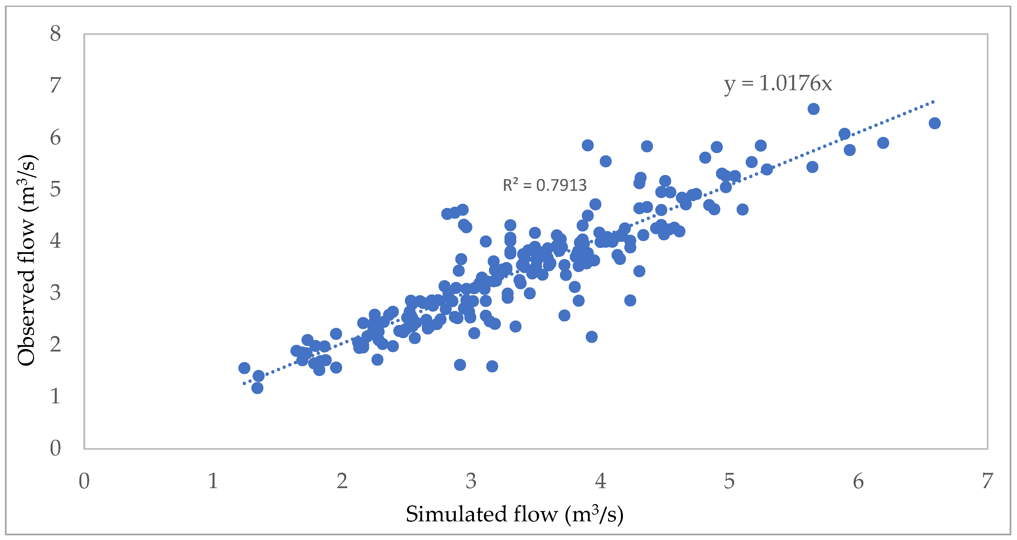
The SWAT model was calibrated in Figure 3 and Figure 4 having a coefficient of determination (R²), Nash–Sutcliffe efficiency (NSE), mean percentage error, mean absolute percentage error and percent bias (PBIAS) values of 0.8, 0.76, 0.69, 10.3 and −11.6 during calibration and 0.8, 0.76, 3.9, 11.6 and −3.9 during validation, respectively. The goodness of fit (R², NSE, MPE, MAPE and PBIAS) was found to be very good indicating the performance of the model output for the intended purpose was acceptable. The model performance determined by the Nash-Sutcliff (NSE) was 0.8 during calibration and validation in the study area, which is good for interpreting the model output [5]. Similar results were reported elsewhere [88,89,90] for the model simulation and observation.

The SWAT generated flow at sub-catchment outlet was used to calculate the load in FLUX32. Accordingly, the flow-weighted concentration calculated by method 6 (Equation (4)) was less than 0.2 of all other methods in FLUX32. The residual plot of bias for flow, date and month at each sub-basin outlet in LHW was in the range of 0–0.05, indicating it is acceptable. Similarly, the plot of slope significance was in the range of 0.8–0.99. The recommended coefficient of variation (CV) is in the range of 0–0.2 during flow-weighted load calculation and it is in the range of 0–0.058, showing surprisingly good performance of FLUX32 in the watershed under investigation (Table 7).

Similar trends were also reported by Angello et al. [9] and Belachew et al. [6] in Ethiopia for FLUX32 program simulation performance indicators.

3.2. Calibration of the PLOAD Model

Pollutant loads estimated via selected export coefficients (Table 6) by employing the PLOAD model was used as an initial estimate, whilst loads calculated with FLUX32 at selected sub-basin outlets (monitoring stations) in LHW were used for the PLOAD model calibration. During calibration of PLOAD in Excel Solver, the export coefficients were used as independent variables, and their range of values were considered as constraints to set the upper and lower bounds based on the literature during optimization.

Accordingly, at the initial stage of calibration or pre-optimization, the total percentage error between the model predicted and measured load at all monitoring stations for the investigated pollutant parameters are presented in

Table 8. The total percentage error between measured and simulated load at the initial stage of calibration/pre-optimization and after optimization in all monitoring stations in LHW.

Sub-Basin	COD		BOD5		TDS		TN		TP		PO4-P		NOx-N
	Pre-Optimization	Optimization	Pre-Optimization	Optimization	Pre-Optimization	Optimization	Pre-Optimization	Optimization	Pre-Optimization	Optimization	Pre-Optimization	Optimization	Pre-Optimization	Optimization
MS1	41.54	0.0002	9.5	0.00	798.4	0.01	193.3	0.0001	298.6	0.011	28.7	0.0003	1161	0.004
MS2	41.62	0.0001	1.9	0.00	84.7	0.00	92.8	0.00	33.7	0.0	25.1	0.0001	65.6	0.003
MS3	59.81	0.0003	26.7	0.0003	1062	0.9	251.7	0.003	670	0.001	39.4	0.001	1328	0.037
MS6	90.03	0.0023	87.1	0.001	2419	3.12	254.3	91.97	1001	0.023	99	0.005	1754	63.24
∑abs. error	233	0.003	125.2	0.001	4364	4.03	792.1	92	2003	0.035	192.1	0.006	4309	63.3

. The PLOAD prediction for the COD, BOD₅ and PO₄-P were already relatively accurate before calibration and could be further improved. In contrast, the total relative errors of PLOAD predictions at all monitoring stations for TDS, TN, TP and NOx before optimization were in the order of hundreds or thousands of magnitudes. By optimizing the export coefficients using the solver function, the model error could be reduced considerably.

Still, the PLOAD model underestimated the TDS load at Wedessa (MS3) and Wesha sub-basin (MS1) which are located at the upstream portion of LHW, TN and NOx-N at Tikur-Wuha River catchment outlet (MS6). There is a general trend that the total error increases with the size of the sub-basin. Belachew et al. [6] in Kombolcha catchment and Angello et al. [9] in the Akaki River catchment, Ethiopia, have also come up with similar findings.

For COD, BOD₅, TP, and NOx, the export coefficients after optimization showed significant differences for urban, forest land, range land and cultivated land uses. Wetland, bare land and water bodies showed the least variance in pollutant loading, which could be attributable to decreased area coverage and EC contribution in the watershed. Angello et al. [9] also found similar findings in the Akaki River in Ethiopia.

The pollutant loading estimator was also performed using the mean and median values obtained from the optimized export coefficients. At all monitoring stations, the overall percentage error between the model predicted and measured load was 123.83% for mean and 125.33% for median. Furthermore, the observed PLOAD prediction for both mean and median at monitoring stations demonstrated either an overestimation or underestimation of pollutant loads. As a result, the loads calculated using the mean and median ECs were left out of the equation. Consequently, area-specific ECs has been proven to be a useful technique for estimating pollutant loads in the LHW. For effective pollutant load estimations, Angello et al. [9], Cheruiyot and Muhandiki [91] and Shrestha et al. [15] advised the use of area-specific and local ECs. The optimized EC’s values can be further used for effective management of the nonpoint source pollution in the Watershed. Likewise, the PLOAD was validated for a different data set without change in the optimized export coefficient and showed the model prediction is acceptable with a relatively smaller sum of total errors.

The calibrated pollutant ECs showed that the urban land use showed varying export coefficients as the pollutant loading rate for urban land use for COD, BOD₅, TDS, TP and NOx-N varied with location. The contributions of nonpoint sources among the various urban land uses, as well as the basin’s size, are responsible for the observed spatial differences in ECs (

Table 9. Range of export coefficients after calibration of PLOAD for various land uses in LHW.

Land Uses	Export Coefficient from Literatures, kg ha−1 yr−1
	TN	TP	TDS	BOD5	COD	NOx-N	PO4-P
Agriculture	11.9–62.5	0.02–3.3	62–211.4	42.9–76	68.4–260	0.03–36.1	11.1–14.4
Bare Land	5	0.2	93–100	3.46	5	7–67	4.8–5.1
Range Land	11.6–11.8	0.24–2.64	93.8–100	0.5	0.5	0.46	2
Forest Land	5.85–6	0.43–1.02	167–250	46.6–51	48.3–56	2–2.1	0.7
Urban	36	1.95–2.53	2096–2243	1490–2238	1950–3196	88.2–98.02	1.7
Water Body	0.75	0.2	150	50	50	0.45	10
Wetlands	2.3	0.12–0.15	100–123	5.85	35.5	1.8	0.05

).

The agricultural land use for the calibrated pollutant EC’s showed significant variations among monitoring stations. The contribution of pollutant loading rate for agricultural land for COD, BOD₅, TDS TN and NOx-N demonstrated, the agricultural land use varies spatially in pollutant loading rate contribution. TP and PO₄-P, on the other hand, have revealed a slight variation among the stations.

3.3. Pollutants Flux in LHW by Using PLOAD

The pollutant flux at each of the sub-basin outlets were calculated with the help of FLUX32. A similar approach was also followed by Angello et al. [9], Belachew et al. [6], Xin et al. [92], Liu et al. [56], Gurung et al. [20], Lin and Kleiss, [51], Edwards and Miller [52] and Shen et al. [10]. The estimated pollutant flux at each monitoring stations showed that the organic pollution contribution from the point and nonpoint sources prevailing in the study area, where the maximum COD and BOD₅ load was observed at MS6 with 4976.35 and 3543.54 t/y, respectively (

Table 10. Pollutant flux at catchment outlets of LHW by using PLOAD, t/y.

Catchment Outlets	COD	BOD5	TDS	TN	TP	PO4-P	NOx-N
MS1	635.4	327	659.2	50.9	1.69	49.3	11.2
MS2	531.8	197.1	238.8	43.6	1.09	31.6	7.84
MS3	2665.5	881.8	2229.5	65.9	2.19	115.4	21.1
MS6	4976.4	3543.5	8741.5	149.6	3.28	284.9	43.1

). This station was located downstream of the two-point sources (the BGI effluent discharge site and the Moha soft drinks factory), as well as receiving flow from the upper streams that make a confluence.

Furthermore, at the same monitoring station, the PO₄-P, TN, TP and NOx-N loads were calculated, and the results revealed that the pollutant flux at MS6 (downstream) is greater than the rest of the catchment outlets at upper streams. This is because the land uses at MS6 monitoring stations are dominated by urban lands (large- and small-scale industries), followed by agricultural activities and residential settlements. This river section is highly polluted as most of the untreated household wastes, stormwater runoff from urban and rural areas and industrial effluents are discharged onto it.

The non-point source contribution, on the other hand, was well demonstrated at sub-basins of monitoring stations located in the upper catchment (MS1 to MS3) with the COD and BOD₅ load, as shown in Table 10, indicating that the pollutant flux from non-point sources is significant even if no identified point sources were present. Moreover, the catchments were dominated by agricultural land uses with small urban areas. Similar findings were also reported by the studies conducted by Belachew et al. [6] in Ethiopia and Jain et al. [93] elsewhere. This could be due to relatively small flow and less anthropogenic influence in the upper catchment.

3.4. Pollutant Flux from Point Sources in Hawassa City

Saint George Brewery, BGI (MS4) and Moha soft drinks factory (MS5) have all discharged their effluents into a wetland that feeds the Tikur-Wuha River, which flows into Lake Hawassa. According to the findings of the study, as shown in

Table 11. Point source (PS) loads of selected physicochemical parameters using FLUX 32 in Hawassa City, t/y.

Monitoring Sites	COD	BOD5	TN	TDS	TP	PO4-P	NOx-N
MS4	106.2	25.6	8.9	932.9	7.1	12.3	1.894
MS5	92.0	31.7	3.7	287.6	1.5	11.5	0.074
MS15	14.9	3.3	2.1	93.9	0.2	1.7	0.171
MS19	211.7	53.7	4.3	287.4	0.7	3.6	0.510

, both point sources contributed significant amounts of pollutant loads to the Tikur-Wuha River (MS6) on top of the non-point pollutant loads from the upper catchment that later joined Lake Hawassa.

On the other hand, Referral hospital and Hawassa Industrial Park were two of the point sources that release their effluents in to Lake Hawassa directly. Referral Hospital is the major known single source for pollutant load contribution to lake Hawassa. Additionally, it may threaten the lake by release of various hazardous substances and pollutants, which are not covered by the investigated parameters. Having known the impact of wastes, Hawassa University constructed a waste stabilization ponds (WSP’s) with the intention that the wastewater released are treated based on the discharge standards of the effluents into the water bodies. Nevertheless, the findings of the study revealed that the existing WSP’s is not efficient enough to treat the effluent with the desired treatment level as it contributes huge amount of pollutant loads into the lake. The hospital contributes 14.9 tons COD, 3.3 tons BOD₅, 2.1 tons TN, 93.9 tons TDS, 0.2 tons TP, 1.7 tons PO₄-P and 0.171 tons NOx-N annually. Additionally, Hawassa industrial park was designed initially to comply the zero-emission standard, with no pollutants discharged directly into the Lake. However, during the study periods, huge amounts of pollutants were discharged directly into the Lake as evidenced by personal observation and informal interview. The result on Table 11 showed that Hawassa industrial park contributes COD, BOD₅, TN, TDS, TP, PO₄-P and NOx loads with their annual loads of 211.7, 53.7, 4.3, 287.4, 0.7, 3.6 and 0.51 tons, respectively.

3.5. Estimation of Rainfall Depth for the City of Hawassa

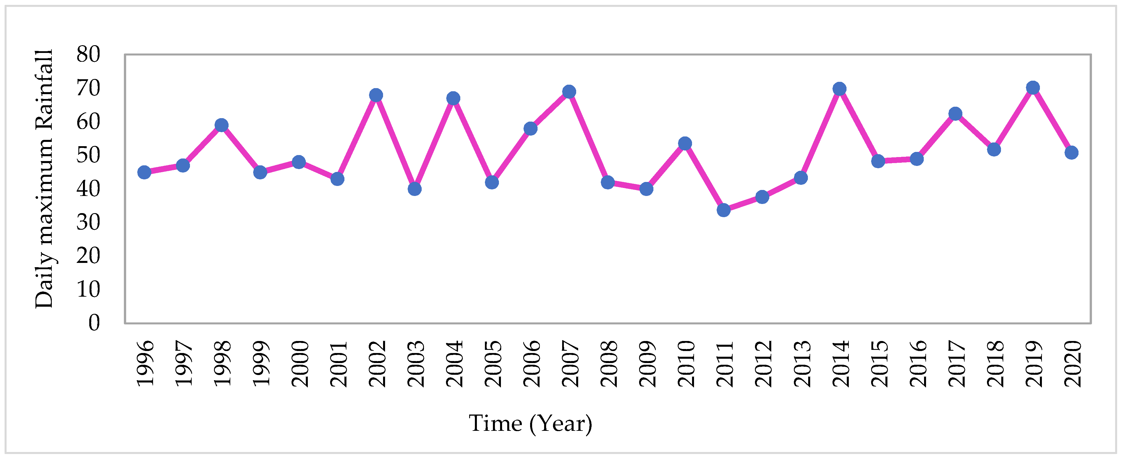
The daily maximum rainfall data for the year 1996 to 2020 (25 years) as shown in Figure 5 was collected from the Ethiopian meteorology agency for Hawassa City.

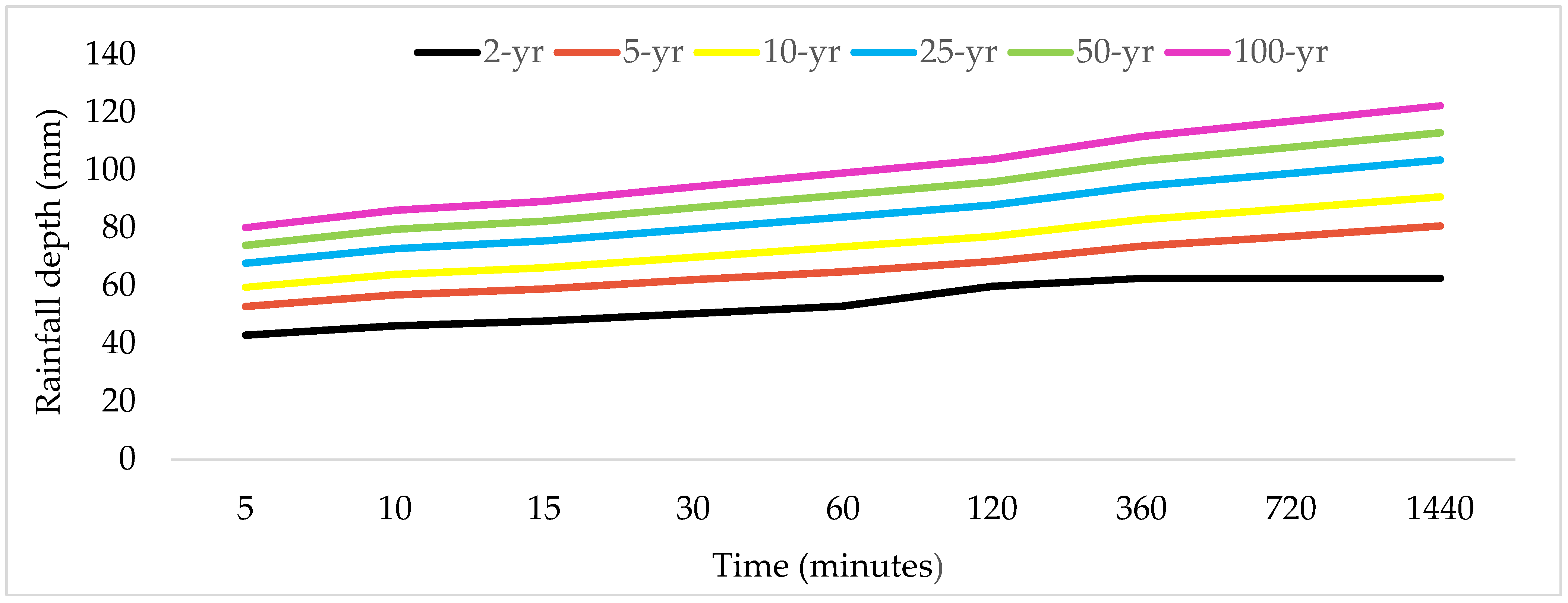
The rainfall depth at different durations was plotted in Figure 6 for short duration rainfall of 5, 10, 15, 30, 60, 120, 360, 720 and 1440 min for a return period of 5, 10, 25, 50 and 100 years by making use of Gumbel’s extreme value distribution and the empirical reduction formula. The rainfall frequency (mm) produced by the 24 h rainfall for 2-year return period (62.7 mm) was then used in the direct runoff determination by SCS-CN method. The obtained result of rainfall frequency of this study in Hawassa City is also in agreement to the intensity duration frequency developed by Ethiopian roads authority for the region containing Hawassa city [66].

3.5.1. Estimation of Curve Number (CN) for the City of Hawassa

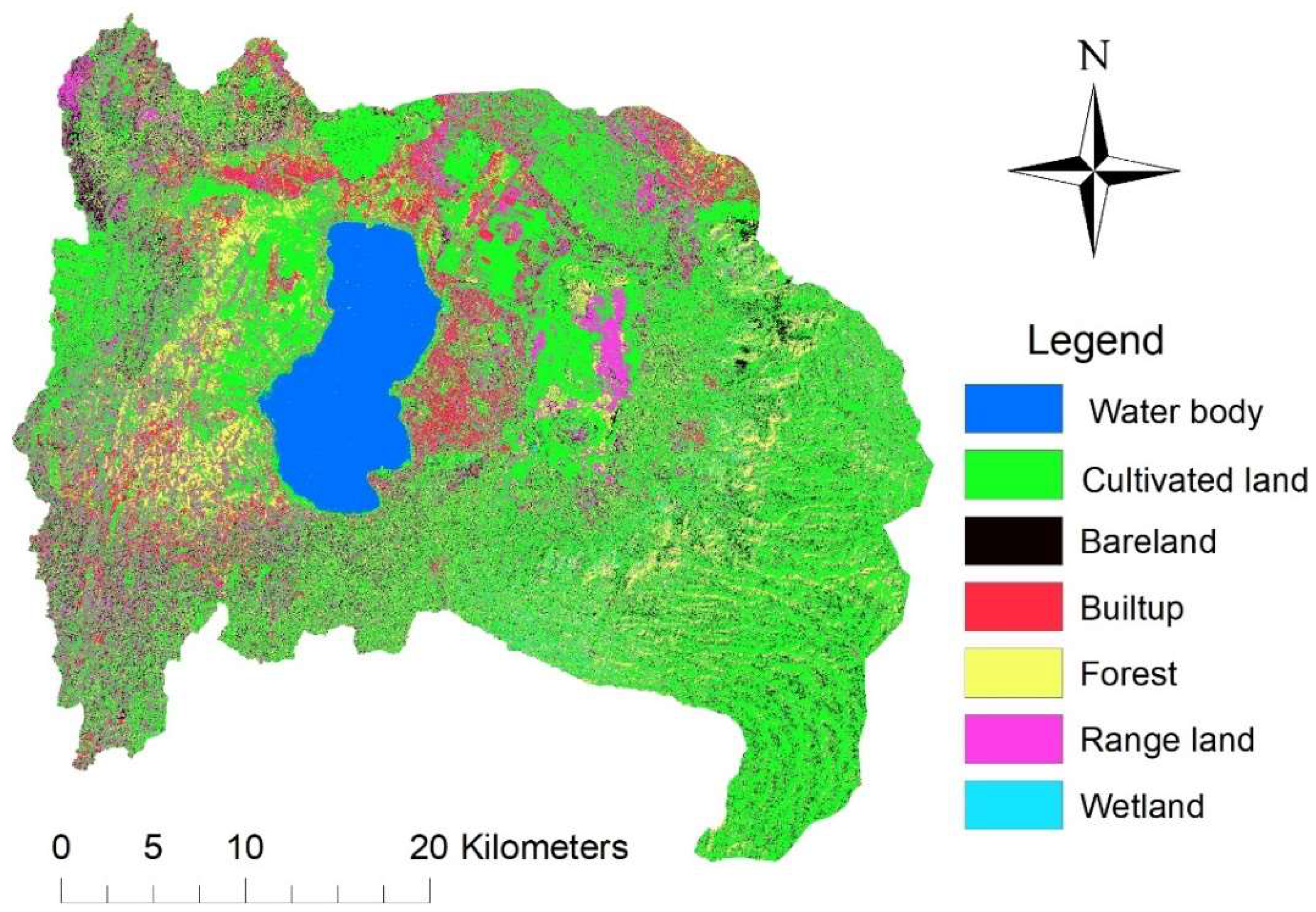
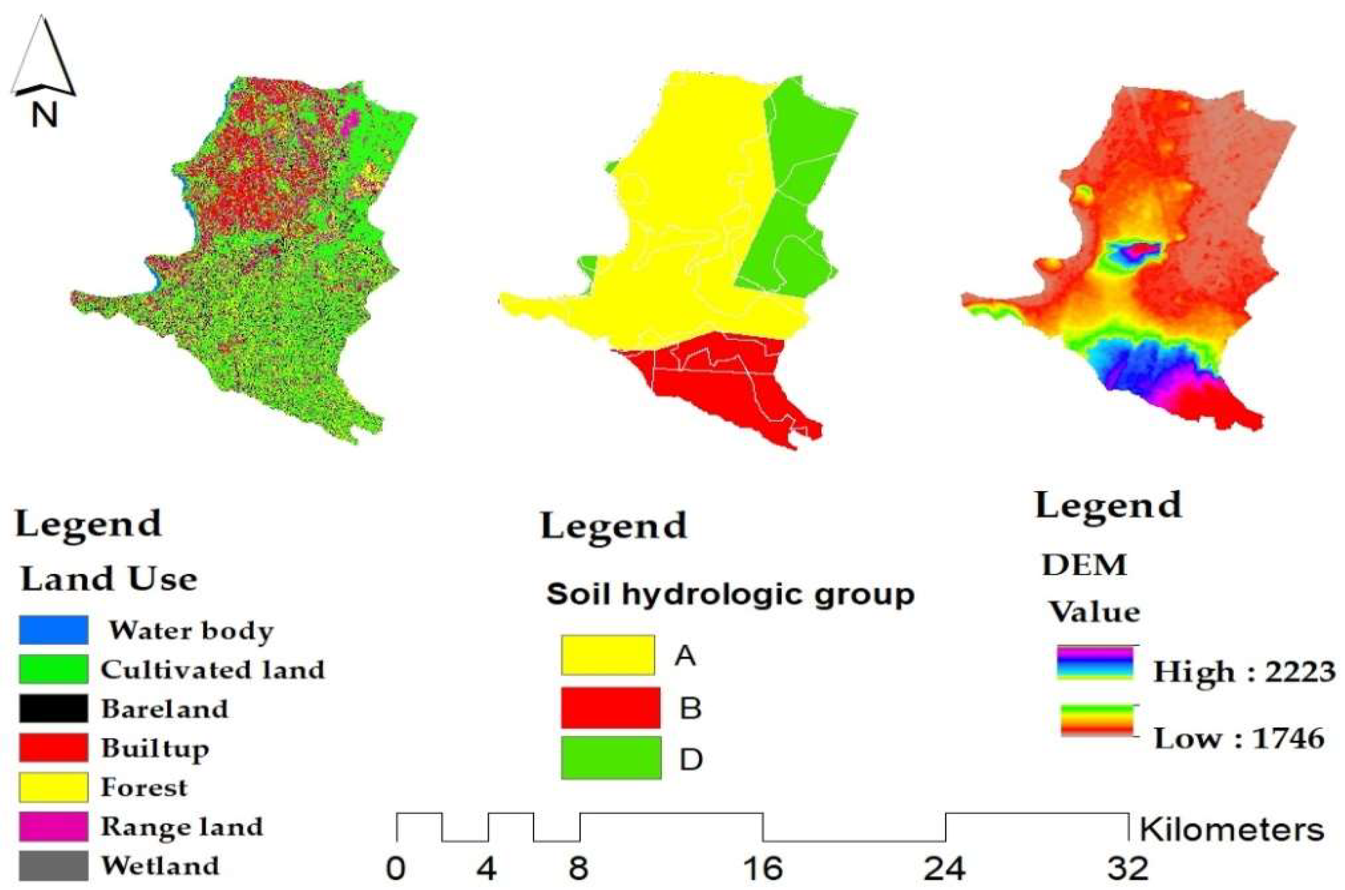
The soil layer, the digital elevation model and land use layers were clipped for Hawassa City. Thereafter, the land use of Hawassa City was reclassified, the hydrologic soil group maps and the land use layer were merged. The CNLookUp table was prepared for land use and sinks in DEM was filled. The land use map, soil hydrologic map and DEM of Hawassa City is shown below in Figure 7.

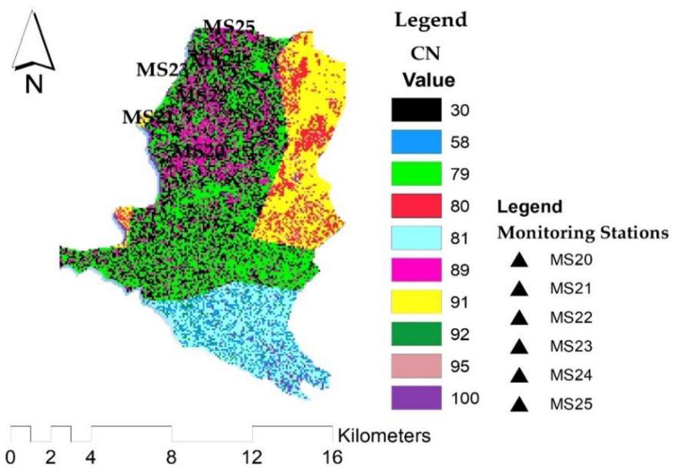
Subsequently, the merged land use and hydrologic soil group maps, DEM and the CNLookUp table were combined to create the CN grid using HEC-GeoHMS following the procedures stated by Merwade [87]. Accordingly, the curve number for monitoring stations in Hawassa City was obtained and used to estimate the runoff depth as shown in Figure 8.

The result showed that the values of CN in Hawassa City ranged from 30–100 indicating high CNs (81–100) corresponding to the urbanized areas of the watershed which has the capability for producing the highest amount of runoff during a storm event. The CN values varies with the subtype of urban land use (i.e., residential, commercial, industrial). Whilst low curve numbers (30–77) corresponding to the forested and cultivated areas that generate little runoff due to high infiltration rate. The result of the study revealed that the CN ranged from 81 for MS21 and MS23 to 89 for MS20, MS22, MS24 and MS25.

3.5.2. Estimation of Runoff Depth for Hawassa City

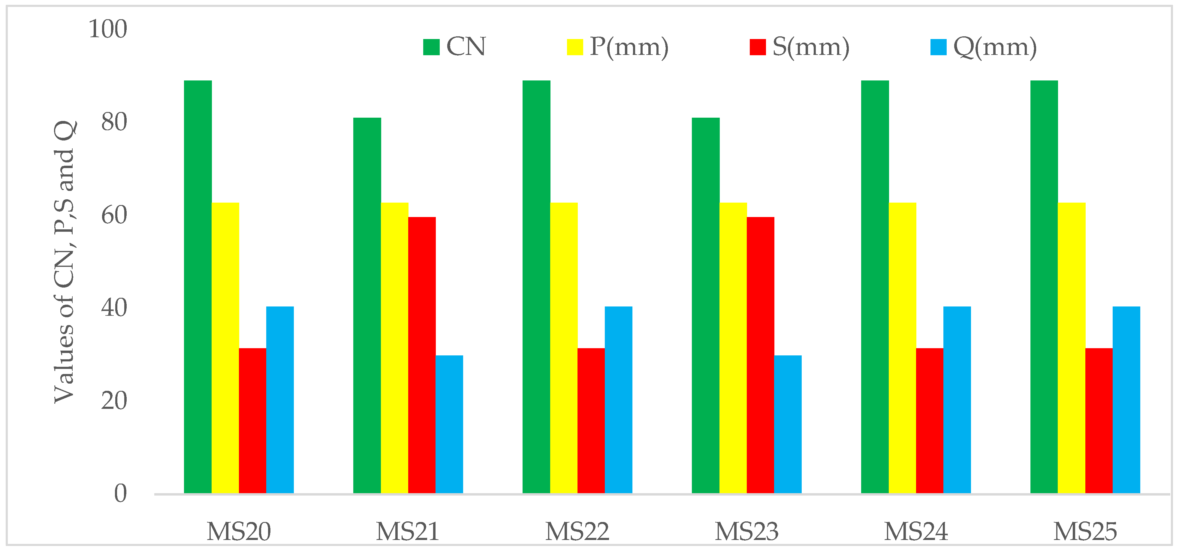
The runoff depth (Q) can be estimated using Equation (15) based on the rainfall frequency produced by the 24-hr rainfall for a two-year return period (Figure 6), curve number (Figure 8) and maximum potential storage Equation (15). As a result, the direct runoff result for the corresponding monitoring stations is depicted in Figure 9.

3.6. Stormwater Pollutant Flux in Hawassa City

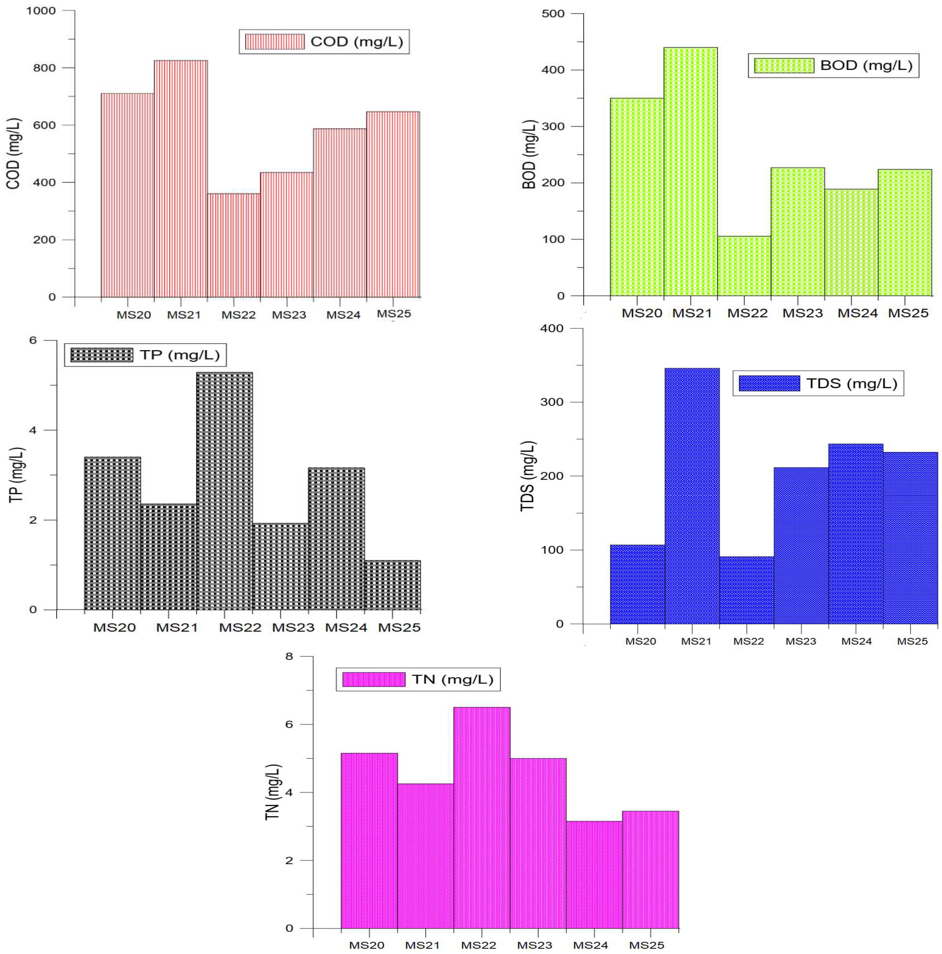
The city of Hawassa has various urban catchments that can convey urban storm runoff with open storm drains and the urban runoff joins the lake at various outfalls. For selected parameters, the stormwater quality characteristics were determined and the results of concentrations of stormwater at monitoring stations were depicted in Figure 10.

The findings of investigations were higher than that of Wondie [93,94], a study conducted in Bahir-dar city, despite the fact that Rădulescu et al. [95] and Li et al. [96] reported comparative findings in Romania and China, respectively. The annual pollutant loads (t/y) for selected physicochemical parameters for each monitoring outfall were estimated utilizing the catchment area (ha) and the corresponding direct runoff determined using the 24 h rainfall frequency (mm) for a two-year return period. As a result, the stormwater pollutant loads of selected physicochemical parameters in Hawassa City were tabulated in tons per year (

Table 12. Stormwater pollutant loads of selected physicochemical parameters in Hawassa City, t/y.

Monitoring Sites	Contributing to	COD	BOD5	TDS	TN	TP
MS20	Lake Hawassa	87.7	43.2	13.2	0.64	0.42
MS21	Lake Hawassa	50.9	27.1	21.3	0.26	0.15
MS22	Lake Hawassa	14.1	4.1	3.6	0.25	0.21
MS23	Lake Hawassa	49	25.6	23.8	0.56	0.22
MS24	Lake Hawassa	22.5	7.2	9.3	0.16	0.12
MS25	Lake Hawassa	32.2	11.2	11.6	0.17	0.05

).

The most heavily contaminated site, according to this research, was MS20 (near Referral Hospital), which encompasses residential settlements, commercial centers and institutions (hotels, restaurants, cafeteria, hospitals). MS21 (near Amora-Gedel) and MS23 (near Chambalala Hotel) sites include residential settlements, businesses and commercial centers, all of which contribute significantly to pollution load. In the Amora-Gedel site, there are resort, hotels, cafeterias, a fish market, a recreation center and Gudumale, where the people of Sidama celebrate their new year festivities. Consequently, a considerable amount of pollutant load was released into the nearby lake during storm occurrences.

4. Conclusions

In this study, we applied a combination of various models (PLOAD, SWAT, FLUX32, HEC-GeoHMS and SCS-CN) with monitoring data to estimate the pollutant flux in the data-limited LHW. The chosen approach was effective in reckoning the annualized diffused source pollution load and is capable to estimate the impact of the spatially distributed emissions on the pollutant flux of receiving streams. It helps to identify the primary source of scattered pollution and provides an effective way for determining organic pollutants and nutrient loads in data-scarce areas.

Estimates of export coefficients from land use in Ethiopia is hardly common and there have been few previous experiences with estimating pollutant loads from the catchments. Thus, transformation of published export coefficients from other studies to characteristics of study area (land use, soil type, slope, climate) was made. In the catchments with no frequent data, estimation of pollutant flux with ECs involved uncertainties. However, the error can be significantly reduced by calibrating with monitored data. Generally, more detailed studies incorporating frequent monitoring of water quality and quantity for the main rivers are advisable to derive the land use specific pollutant loads that better conform to reality.

The estimated pollutant flux at each monitoring stations showed that the organic and nutrient pollutant contribution from the point and nonpoint sources prevailing in the study area, where the maximum pollutant loads were observed at Tikur-Wuha sub-catchments. This station was located downstream of the two-point sources and received flow from the upper streams where agricultural use is predominant. The integration of HEC-GeoHMS and SCS-CN with the catchment area enabled to determine stormwater pollution load of Hawassa City. Accordingly, Hawassa city has been identified as a key pollutant load driver, owing to increased impacts from clearly identified point sources and stormwater pollutant flux from major outfalls. Agricultural activities, on the other hand, cover a large portion of the catchment and are a considerable contributor to the overall load that reaches the lake. Thus, mitigation measures that are focused on pollutant flux reduction to the lake Hawassa have to target the urban and agricultural activities.

References

1. Wang, Q.; Li, S.; Jia, P.; Qi, C.; Ding, F. A review of surface water quality models. Sci. World J. 2013, 2013, 7. [Google Scholar] [CrossRef] [Green Version]
2. Obropta, C.C.; Niazi, M.; Kardos, J.S. Application of an environmental decision support system to a water quality trading program affected by surface water diversions. Environ. Manag. 2008, 42, 946–956. [Google Scholar] [CrossRef]
3. Rode, M.; Arhonditsis, G.; Balin, D.; Kebede, T.; Krysanova, V.; Van Griensven, A.; Van Der Zee, M. New challenges in integrated water quality modelling. Hydrol. Process. 2010, 24, 3447–3461. [Google Scholar] [CrossRef]
4. Kumar, A.; Sharma, M.P.; Rai, S.P. A novel approach for river health assessment of chambal using fuzzy modeling, India. Desalin. Water Treat. 2017, 58, 72–79. [Google Scholar] [CrossRef]
5. Aga, A.O.; Melesse, A.M.; Chane, B. Estimating the sediment flux and budget for a data limited rift valley lake in Ethiopia. Hydrology 2019, 6, 1. [Google Scholar] [CrossRef] [Green Version]
6. Zinabu, E.; van der Kwast, J.; Kelderman, P.; Irvine, K. Estimating total nitrogen and phosphorus losses in a data-poor Ethiopian catchment. J. Environ. Qual. 2017, 46, 1519–1527. [Google Scholar] [CrossRef] [PubMed]
7. Lencha, S.M.; Tränckner, J.; Dananto, M. Assessing the Water Quality of Lake Hawassa Ethiopia—Trophic State and Suitability for Anthropogenic Uses—Applying Common Water Quality Indices. Int. J. Environ. Res. Public Health 2021, 18, 8904. [Google Scholar] [CrossRef] [PubMed]
8. Amare, T.A.; Yimer, G.T.; Workagegn, K.B. Assessment of Metals Concentration in Water, Sediment and Macrophyte Plant Collected from Lake Hawassa, Ethiopia. J. Environ. Anal. Toxicol. 2014, 5, 1000247. [Google Scholar] [CrossRef] [Green Version]
9. Angello, Z.A.; Behailu, B.M.; Tränckner, J. Integral application of chemical mass balance and watershed model to estimate point and nonpoint source pollutant loads in data-scarce little akaki river, Ethiopia. Sustainability 2020, 12, 7084. [Google Scholar] [CrossRef]
10. Shen, Z.; Hong, Q.; Chu, Z.; Gong, Y. A framework for priority non-point source area identification and load estimation integrated with APPI and PLOAD model in Fujiang Watershed, China. Agric. Water Manag. 2011, 98, 977–989. [Google Scholar] [CrossRef]
11. Ding, X.; Shen, Z.; Hong, Q.; Yang, Z.; Wu, X.; Liu, R. Development and test of the Export Coefficient Model in the Upper Reach of the Yangtze River. J. Hydrol. 2010, 383, 233–244. [Google Scholar] [CrossRef]
12. Johnes, P.J. Evaluation and management of the impact of land use change on the nitrogen and phosphorus load delivered to surface waters: The export coefficient modelling approach. J. Hydrol. 1996, 183, 323–349. [Google Scholar] [CrossRef]
13. Neill, D.B.; Moore, A.W.; Pereira, F.; Mitchell, T. Detecting significant multidimensional spatial clusters. Adv. Neural Inf. Process. Syst. 2005. Available online: https://www.cs.cmu.edu/~tom/sss-nips04.pdf (accessed on 19 April 2022).
14. Reckhow, K.H.; Beaulac, M.N.; Simpson, J.T. Modeling phosphorus loading response under uncertain. A manual and compilation of export coefficients. Water Resour. Res. 1980, 30, 214. [Google Scholar]
15. Shrestha, S.; Kazama, F.; Newham, L.T.H.; Babel, M.S.; Clemente, R.S.; Ishidaira, H.; Nishida, K.; Sakamoto, Y. Catchment Scale Modelling of Point Source and Non-Point Source Pollution Loads Using Pollutant Export Coefficients Determined from Long-Term In-Stream Monitoring Data. J. Hydro-Environ. Res. 2008, 2, 134–147. Available online: https://www.sciencedirect.com/science/article/abs/pii/S1570644308000233 (accessed on 23 December 2019). [CrossRef]
16. Rast, W.; Lee, G. Nutrient Loading Estimates for Lakes. J. Environ. Eng. 1983, 109, 502–517. [Google Scholar] [CrossRef] [Green Version]
17. Bowes, M.J.; Smith, J.T.; Jarvie, H.P.; Neal, C. Modelling of phosphorus inputs to rivers from diffuse and point sources. Sci. Total Environ. 2008, 395, 125–138. [Google Scholar] [CrossRef] [Green Version]
18. Scheren, P.; Zanting, H.A.; Lemmens, A.M.C. Estimation of water pollution sources in Lake Victoria, East Africa: Application and elaboration of the rapid assessment methodology. J. Environ. Manag. 2000, 58, 235–248. [Google Scholar] [CrossRef]
19. Wu, L.; Gao, J.; Ma, X. Application of modified export coefficient method on the load estimation of non-point source nitrogen and phosphorus pollution of soil and water loss in semiarid regions. Environ. Sci. Pollut. Res. 2015, 22, 10647–10660. [Google Scholar] [CrossRef]
20. Gurung, D.P.; Githinji, L.J.M.; Ankumah, R.O. Assessing the nitrogen and phosphorus Loading in the Alabama (USA) River Basin Using pLOAD Model. Air Soil Water Res. 2013, 6, 23–36. [Google Scholar] [CrossRef]
21. Povilaitis, A. Source apportionment and retention of nutrients and organic matter in the Merkys River basin in southern Lithuania. J. Environ. Eng. Landsc. Manag. 2008, 16, 195–204. [Google Scholar] [CrossRef]
22. Fleifle, A.; Saavedra, O.; Yoshimura, C.; Elzeir, M.; Tawfik, A. Optimization of integrated water quality management for agricultural efficiency and environmental conservation. Environ. Sci. Pollut. Res. 2014, 21, 8095–8111. [Google Scholar] [CrossRef] [PubMed]
23. Amaya, F.L.; Gonzales, T.A.; Hernandez, E.C.; Luzano, E.V.; Mercado, N.P. Estimating Point and Non-Point Sources of Pollution in Biñan River Basin, the Philippines. APCBEE Procedia 2012, 1, 233–238. [Google Scholar] [CrossRef] [Green Version]
24. Wali, U.G.; Nhapi, I.; Ngombwa, A.; Banadda, N.; Nsengimana, H.; Kimwaga, R.J.; Nansubuga, I. Modelling of Nonpoint Source Pollution in Akagera Transboundary River in Rwanda. Open Environ. Eng. J. 2011, 4, 124–132. [Google Scholar] [CrossRef] [Green Version]
25. Sishah, S. Rainfall runoff estimation using GIS and SCS-CN method for awash river basin, Ethiopia. Int. J. Hydrol. 2021, 5, 33–37. [Google Scholar] [CrossRef]
26. Verma, S.; Mishra, S.K.; Verma, R.K. Improved runoff curve numbers for a large number of watersheds of the USA. Hydrol. Sci. J. 2020, 65, 2658–2668. [Google Scholar] [CrossRef]
27. Awulachew, S.B. Investigation of physical and bathymetric characteristics of Lakes Abaya and Chamo, Ethiopia, and their management implications. Lakes Reserv. Res. Manag. 2006, 11, 133–140. [Google Scholar] [CrossRef]
28. Lencha, S.M.; Ulsido, M.D.; Muluneh, A. Evaluation of Seasonal and Spatial Variations in Water Quality and Identification of Potential Sources of Pollution Using Multivariate Statistical Techniques for Lake Hawassa. Appl. Sci. 2021, 11, 8991. [Google Scholar] [CrossRef]
29. Abebe, Y.; Bitew, M.; Ayenew, T.; Alo, C.; Cherinet, A.; Dadi, M. Morphometric change detection of Lake Hawassa in the Ethiopian Rift Valley. Water 2018, 10, 625. [Google Scholar] [CrossRef] [Green Version]
30. Wondrade, N.; Dick, Ø.B.; Tveite, H. GIS based mapping of land cover changes utilizing multi-temporal remotely sensed image data in Lake Hawassa Watershed, Ethiopia. Environ. Monit. Assess. 2014, 186, 1765–1780. [Google Scholar] [CrossRef]
31. American Public Health Association; American Water Works Association; Water Environment Federation. Standard Methods for the Examination of Water and Wastewater, 23rd ed.; American Public Health Association: Washington, DC, USA, 2017. [Google Scholar]
32. Grubbs, F.E. Procedures for Detecting Outlying Observations in Samples. Technometrics 2011, 11, 1–21. [Google Scholar] [CrossRef]
33. Suhaimi, N.; Ghazali, N.A.; Nasir, M.Y.; Mokhtar, M.I.; Ramli, N.A. Markov Chain Monte Carlo Method for Handling Missing Data in Air Quality Datasets. Malays. J. Anal. Sci. 2017, 21, 552–559. [Google Scholar] [CrossRef]
34. Gassman, P.W.; Reyes, M.R.; Green, C.H.; Arnold, J.G. The soil and water assessment tool: Historical development, applications, and future research directions. Trans. ASABE 2007, 50, 1211–1250. [Google Scholar] [CrossRef] [Green Version]
35. Arnold, J.G.; Srinivasan, R.; Muttiah, R.S.; Williams, J.R. Large area hydrologic modeling and assessment Part I: Model Development’ basin scale model called SWAT (Soil and Water speed and storage, advanced software debugging policy to meet the needs, and the management to the tank model. JAWRA J. Am. Water Resour. Assoc. 1998, 34, 73–89. [Google Scholar] [CrossRef]
36. Saka, F.; Babacan, H.T. Discharge Estimation by Drainage Area Ratio Method at Some Specific Discharges for 2251 Stream Gauging Station in East Black Sea Basin, Turkey. Transp. Traffic Serv. Progr. 2019, 2, 22–25. [Google Scholar]
37. Shu, C.; Ouarda, T.B.M.J. Improved methods for daily streamflow estimates at ungauged sites. Water Resour. Res. 2012, 48, W02523. [Google Scholar] [CrossRef]
38. Borah, D.K.; Bera, M. Watershed Scale Hydrologic and Non-Point Source Pollution Models: Review of Applications. Trans. ASAE 2004, 47, 789. [Google Scholar] [CrossRef] [Green Version]
39. Singh, K.P.; Malik, A.; Sinha, S. Water quality assessment and apportionment of pollution sources of Gomti river (India) using multivariate statistical techniques—A case study. Anal. Chim. Acta 2005, 538, 355–374. [Google Scholar] [CrossRef]
40. Karki, R.; Tagert, M.L.M.; Paz, J.O.; Bingner, R.L. Application of AnnAGNPS to model an agricultural watershed in East-Central Mississippi for the evaluation of an on-farm water storage (OFWS) system. Agric. Water Manag. 2017, 192, 103–114. [Google Scholar] [CrossRef]
41. Haith, D.A.; Mandel, R.; Wu, R.S. GWLF, Generalized Watershed Loading Functions Version 2.0 User’s Manual; Department of Agricultural and Biological Engineering, Cornell University: Ithaca, NY, USA, 1992. [Google Scholar]
42. Behrendt, H.; Venohr, M.; Hirt, U.; Hofmann, J.; Opitz, D.; Andreas, G. The Model System MONERIS User’s Manual Version 2.0; Leibniz-Institute of Freshwater Ecology and Inland Fisheries: Berlin, Germany, 2007. [Google Scholar]
43. DHI. A Modelling System for Rivers and Channels Reference Manual for MIKE11. 2017. Available online: http://10.0.46.73/zrzyxb.20160781%0Ahttps://search.ebscohost.com/login.aspx?direct=true&db=a9h&AN=125384783&site=ehost-live&scope=site (accessed on 12 August 2021).
44. Linfield, C.B.; Barnwell, T. The Enhanced Stream Water Quality Models QUAL2E and QUAL2E—UNCAS Documentation and User Manual; United States Environmental Protection Agency: Athens, GA, USA, 1987.
45. Smith, R.A.; Schwarz, G.E.; Alexander, R.B. Regional interpretation of water-quality monitoring data. Water Resour. Res. 1997, 33, 2781–2798. [Google Scholar] [CrossRef] [Green Version]
46. Brian, R.B.; Imhoff, J.C.; Kittle, J.L.; Jobes, T.H.; Donigian, A.S. Hydrological Simulation Program—Fortran (HSPF) User’s Manual Version 12; Hydrologic Analysis Software Support Program Office of AQUA TERRA Consultants: Mountain View, CA, USA, 2001; pp. 1–873. [Google Scholar]
47. USEPA. BASINS 4.5 Better assessment science integrating point and non-point Sources. Am. J. Orthod. Dentofac. Orthop. 2019, 155, 145.e1–145.e2. [Google Scholar] [CrossRef]
48. Lai, Y.C.; Yang, C.P.; Hsieh, C.Y.; Wu, C.Y.; Kao, C.M. Evaluation of non-point source pollution and river water quality using a multimedia two-model system. J. Hydrol. 2011, 409, 583–595. [Google Scholar] [CrossRef]
49. Ambrose, R.B.; Wool, T.A.; Martin, J.L. The Water Quality Analysis Simulation Program, Wasp5, Part A: Model Documentation. Environ. Res. Lab. 1992, 1–252. Available online: https://www.researchgate.net/publication/242557430 (accessed on 23 August 2021).
50. Yuan, L.; Sinshaw, T.; Forshay, K.J. Review of watershed-scale water quality and nonpoint source pollution models. Geosciences 2020, 10, 25. [Google Scholar] [CrossRef] [Green Version]
51. Lin, J.P.; Kleiss, B.A. Availability of a PowerPoint-Based for Wetlands Management; United States Army Engineer Research and Development Center: Vicksburg, MS, USA, 2004. [Google Scholar]
52. Edwards, C.; Miller, M. An ArcView GIS Tool to Calculate Nonpoint Sources of Pollution in Watershed and Stormwater Projects—Version 3.0; United States Environmental Protection Agency: Washington, DC, USA, 2001; pp. 1–48. Available online: http://water.epa.gov/scitech/datait/models/basins/upload/2002_05_10_BASINS_b3docs_PLOAD_v3.pdf (accessed on 20 September 2021).
53. Anderson, J.R.; Hardy, E.E.; Roach, J.T.; Witmer, E.R. A Land Use and Land Cover Classification System for Use with Remote Sensor Data; U.S. Geological Survey: Alexandria, VA, USA, 1976.
54. Li, S.; Zhang, L.; Du, Y.; Liu, H.; Zhuang, Y.; Liu, S. Evaluating Phosphorus Loss for Watershed Management: Integrating a Weighting Scheme of Watershed Heterogeneity into Export Coefficient Model. Environ. Model. Assess. 2016, 21, 657–668. [Google Scholar] [CrossRef]
55. Liu, R.; Yu, W.; Shi, J.; Wang, J.; Xu, F.; Shen, Z. Development of regional pollution export coefficients based on artificial rainfall experiments and its application in North China. Int. J. Environ. Sci. Technol. 2016, 14, 823–832. [Google Scholar] [CrossRef]
56. Liu, R.; Yang, Z.; Shen, Z.; Yu, S.L.; Ding, X.; Wu, X.; Liu, F. Estimating nonpoint source pollution in the upper Yangtze River using the export coefficient model, remote sensing, and geographical information system. J. Hydraul. Eng. 2009, 135, 698–704. [Google Scholar] [CrossRef]
57. Delkash, M.; Al-Faraj, F.A.M.; Scholz, M. Comparing the export coefficient approach with the soil and water assessment tool to predict phosphorous pollution: The Kan watershed case study. Water Air Soil Pollut. 2014, 225, 2122. [Google Scholar] [CrossRef]
58. Clesceri, N.L.; Curran, S.J.; Sedlak, R.I. Nutrient Loads To Wisconsin Lakes: Part I. Nitrogen and Phosphorus Export Coefficients. JAWRA J. Am. Water Resour. Assoc. 1986, 22, 983–990. [Google Scholar] [CrossRef]
59. Povilaitis, A. Nutrient retention in surface waters of Lithuania. Pol. J. Environ. Stud. 2011, 20, 1575–1584. [Google Scholar]
60. Lin, J.P. Review of Published Export Coefficient and Event Mean Concentratoin (EMC) Data. Wetl. Regul. Assist. Progr. 2004, 15. Available online: http://www.dtic.mil/cgi-bin/GetTRDoc?AD=ADA430436 (accessed on 10 January 2022).
61. Jeje, Y. Export Coefficients for Total Phosphorus, Total Nitrogen and Total Suspended Solids in the Southern Alberta Region: A Review of Literature; University of Alberta Libraries: Calgary, AB, Canada, 2016. [Google Scholar]
62. Walker, W.W. Simplified Procedures for Eutrophication Assessment and Prediction: User Manual; United States Army Corps of Engineers: Vicksburg, MS, USA, 1999.
63. Walker, W.W. Environmental and Water Quality Operational Studies; Empirical Methods for Predicting Eutrophication in Impoundments; U.S. Army Engineer Waterways Experiment Station: Vicksburg, MS, USA, 1987. [Google Scholar]
64. Saleh, S. Solving Linear Programming Problems by Using Excel’s Solver. Tikrit J. Pure Sci. 2009, 14, 87–98. Available online: https://www.researchgate.net/publication/332513460 (accessed on 5 January 2022).
65. Troxell, D.S. Optimization Software Pitfalls: Raising Awareness in the Classroom. INFORMS Trans. Educ. 2002, 2, 40–46. [Google Scholar] [CrossRef] [Green Version]
66. ERA. Drainage Design Manual; Ethiopian Roads Authority: Addis Ababa, Ethiopia, 2013.
67. Jemberie, M.A.; Melesse, A.M. Urban Flood Management through Urban Land Use Optimization Using LID Techniques, City of Addis Ababa, Ethiopia. Water 2021, 13, 1721. [Google Scholar] [CrossRef]
68. Tilahun, B.Z. Hydraulic Performance Assessment of Storm Water Drainage Systems of Dejen Town Using Storm Water Management Model (SWMM), Ethiopia. GSJ 2021, 9, 1358–1383. [Google Scholar]
69. Gerezihier, Y. Development of rainfall intensity-duration-frequency (IDF) relationships for Siti Zone, in case of Ethiopia Somali Regional State. Civ. Environ. Res. 2019, 9, 10–28. [Google Scholar]
70. Elsebaie, I.H. Developing rainfall intensity–duration–frequency relationship for two regions in Saudi Arabia. J. King Saud Univ.-Eng. Sci. 2012, 24, 131–140. [Google Scholar] [CrossRef] [Green Version]
71. Mohammed, J.I.; Kumsa, G. Developing Rainfall Intensity Duration Curve for Selected Towns in Western Part of Ethiopia. Hydrology 2021, 9, 56. [Google Scholar] [CrossRef]
72. Thein, S.H. Modelling of Short Duration Rainfall IDF Equation. Am. Sci. Res. J. Eng. Technol. Sci. 2019, 58, 17–19. [Google Scholar]
73. NEHP630. National Engineering Handbook Chapter 7 Hydrologic Soil Groups; USDA-SCS: Washington, DC, USA, 2009. [Google Scholar]
74. Bunganaen, W.; Frans, J.H.; Seran, Y.A.; Legono, D.; Krisnayanti, D.S. Rainfall-Runoff Simulation Using HEC-HMS Model in the Benanain Watershed, Timor Island. J. Civ. Eng. Forum. 2021, 7, 359. [Google Scholar] [CrossRef]
75. Santikari, V.P.; Murdoch, L.C. Including effects of watershed heterogeneity in the curve number method using variable initial abstraction. Hydrol. Earth Syst. Sci. 2018, 22, 4725–4743. [Google Scholar] [CrossRef] [Green Version]
76. Krajewski, A.; Sikorska-Senoner, A.E.; Hejduk, A.; Hejduk, L. Variability of the initial abstraction ratio in an urban and an agroforested catchment. Water 2020, 12, 415. [Google Scholar] [CrossRef] [Green Version]
77. Li, C.; Liu, M.; Hu, Y.; Shi, T.; Zong, M.; Walter, M. Assessing the impact of urbanization on direct runoff using improved composite CN method in a large urban area. Int. J. Environ. Res. Public Health 2018, 15, 775. [Google Scholar] [CrossRef] [PubMed] [Green Version]
78. Im, S.; Lee, J.; Kuraji, K.; Lai, Y.; Tuankrua, V.; Nobuaki, T.; Gomyo, M.; Inoue, H.; Tseng, C. Soil conservation service curve number determination for forest cover using rainfall and runoff data in experimental forests. J. For. Res. 2020, 25, 204–213. [Google Scholar] [CrossRef]
79. Hawkins, R.H. Asymptotic determination of runoff curve numbers from data. J. Irrig. Drain. Eng. 1993, 1, 117–125. [Google Scholar] [CrossRef]
80. Hawkins, R.H.; Ward, T.J.; Woodward, E.; Van Mullem, J.A. Continuing evolution of rainfall-runoff and the curve number precedent. In Proceedings of the 2nd Joint Federal Interagency Conference, Las Vegas, NV, USA, 27 June–1 July 2010; pp. 2–12. [Google Scholar]
81. Woodward, D.E.; Hawkins, R.H.; Ruiyun, J.; Hjelmfelt, A.T.; Mullem, J.A.; Quan, Q.D. Runoff curve number method: Examination of the initial abstraction ratio. World Water Congr. 2003, 2003, 1–10. [Google Scholar]
82. Assaye, H.; Nyssen, J.; Poesen, J.; Lemma, H.; Meshesha, D.T.; Wassie, A.; Adgo, E.; Frankl, A. Curve number calibration for measuring impacts of land management in sub-humid Ethiopia. J. Hydrol. Reg. Stud. 2021, 35, 100819. [Google Scholar] [CrossRef]
83. Ajmal, M.; Waseem, M.; Kim, D.; Kim, T. A pragmatic slope-adjusted curve number model to reduce uncertainty in predicting flood runoff from steep watersheds. Water 2020, 12, 1469. [Google Scholar] [CrossRef]
84. Jahan, K.; Pradhanang, S.M.; Bhuiyan, M.A.E. Surface runoff responses to suburban growth: An integration of remote sensing, GIS, and curve number. Land 2021, 10, 452. [Google Scholar] [CrossRef]
85. Shukur, H.K. Estimation Curve Numbers Using GIS and Hec-GeoHMS Model. J. Eng. 2017, 23, 1–11. Available online: https://joe.uobaghdad.edu.iq/index.php/main/article/view/37 (accessed on 16 November 2021).
86. Dwivedi, K.; Tripathi, M. Preparation of Curve Number Map for hydrologic simulation using GIS and HEC-Geo-HMS Model. Int. J. Curr. Microbiol. Appl. Sci. 2020, 9, 3264–3270. [Google Scholar] [CrossRef]
87. Merwade, V. Creating SCS Curve Number Grid using HEC-GeoHMS. Sch. Civ. Eng. Purdue Univ. 2012, 1–15. Available online: http://www.hec.usace.army.mil/software/hec-geohms/downloadlink.html (accessed on 16 November 2021).
88. Paul, S.; Cashman, M.A.; Szura, K.; Pradhanang, S.M. Assessment of nitrogen inputs into hunt river by onsite wastewater treatment systems via SWAT simulation. Water 2017, 9, 610. [Google Scholar] [CrossRef] [Green Version]
89. Narsimlu, B.; Gosain, A.K.; Chahar, B.R.; Singh, S.K.; Srivastava, P.K. SWAT Model Calibration and Uncertainty Analysis for Streamflow Prediction in the Kunwari River Basin, India, Using Sequential Uncertainty Fitting. Environ. Process. 2015, 2, 79–95. [Google Scholar] [CrossRef]
90. Mengistu, A.G.; van Rensburg, L.D.; Woyessa, Y.E. Techniques for calibration and validation of SWAT model in data scarce arid and semi-arid catchments in South Africa. J. Hydrol. Reg. Stud. 2019, 25, 100621. [Google Scholar] [CrossRef]
91. Cheruiyot, C.K.; Muhandiki, V.S. Estimation of Nutrient Export Coefficients in Lake Victoria Basin. J. Water Environ. Technol. 2014, 12, 231–244. [Google Scholar] [CrossRef] [Green Version]
92. Xin, X.; Yin, W.; Li, K. Estimation of non-point source pollution loads with flux method in Danjiangkou Reservoir area, China. Water Sci. Eng. 2017, 10, 134–142. [Google Scholar] [CrossRef]
93. Jain, C.K.; Singhal, D.C.; Sharma, M.K. Estimating nutrient loadings using chemical mass balance approach. Environ. Monit. Assess. 2007, 134, 385–396. [Google Scholar] [CrossRef]
94. Wondie, T.A. The Impact of Urban Storm Water Runoff and Domestic Waste; Cornell University: Ithaca, NY, USA, 2009. [Google Scholar]
95. Rǎdulescu, D.; Racoviţeanu, G.; Swamikannu, X. Comparison of urban residential storm water runoff quality in Bucharest, Romania with international data. In Proceedings of the E3S Web of Conferences, Salé, Morocco, 20 October 2019; Volume 85. [Google Scholar] [CrossRef] [Green Version]
96. Li, D.; Wan, J.; Ma, Y.; Wang, Y.; Huang, M.; Chen, Y. Stormwater runoff pollutant loading distributions and their correlation with rainfall and catchment characteristics in a rapidly industrialized city. PLoS ONE 2015, 10, e0118776. [Google Scholar] [CrossRef]
Figure 1. Study area map and monitoring station’s location. (a) Lake Hawassa watershed (LHW) and monitoring stations from point source (PS), rivers and stormwater, (a) Major river basins in Ethiopia, (b) countries sharing boundaries with Ethiopia (c).
Water 14 01569 g001
Figure 2. Land Use map of Lake Hawassa Watershed.
Water 14 01569 g002
Figure 3. Observed and simulated average monthly flow for Lake Hawassa watershed (calibration and validation).
Water 14 01569 g003
Figure 4. Best fit curve for flow calibration and validation.
Water 14 01569 g004
Figure 5. Daily maximum rainfall depth (mm) from 1996 to 2020 for Hawassa city.
Water 14 01569 g005
Figure 6. Rainfall depth at different durations (minutes) estimated from Gumbel’s extreme value distribution and Ethiopian Roads Authority for Hawassa city.
Water 14 01569 g006
Figure 7. The land use map, soil hydrologic map and DEM of Hawassa City.
Water 14 01569 g007
Figure 8. Curve number for stormwater samples collected over six (n = 6) monitoring stations in Hawassa City.
Water 14 01569 g008
Figure 9. The runoff depth (mm) for the stormwater samples collected over six monitoring stations in Hawassa City.
Water 14 01569 g009
Figure 10. Selected physicochemical parameters concentrations (mg/L) in the stormwater samples collected over six monitoring stations from Hawassa City.
Water 14 01569 g010