
Health-Aware Economic MPC for Operational Management of Flow-Based Networks Using Bayesian Networks


Abstract
:1. Introduction
2. EMPC for DWN
2.1. Control-Oriented Model
2.2. Optimization Problem Formulation
- Economic objective: the economical costs that involve the flow transport while providing the demanded volume should be minimized. This cost function corresponds to:where is the price per volume unit, including the fixed costs related to the supply flow and the variable costs related to the time-varying electricity associated cost. is a diagonal positive definite matrix that is used as a weight to prioritize the terms in the complete objective function.
- Safety objective: the storage devices should guarantee some safety volume to deal with unexpected variations in the demand. This goal can be formulated as follows:where indicates the storage safety volume. However, this piecewise linear formulation can be avoided by considering that the safety cost function can be expressed through a soft constraint by using a slack variable like:and also being introduced as an objective term to retain feasibility of the optimization problem:where is a diagonal positive definite matrix that is used as a weight to prioritize the terms in the complete objective function.
- Smoothness objective: to avoid overloads in the pipes, and preserve the network components lifetime, the actuators are managed based on smooth control actions. To achieve this smoothing effect, the variation of the control actions among two consecutive time instants is penalized as follows:where , and is a diagonal positive definite matrix that is used as a weight to prioritize the terms in the complete objective function.
3. Reliability-Aware Economic MPC Using Bayesian Network Approach
3.1. Bayesian Model
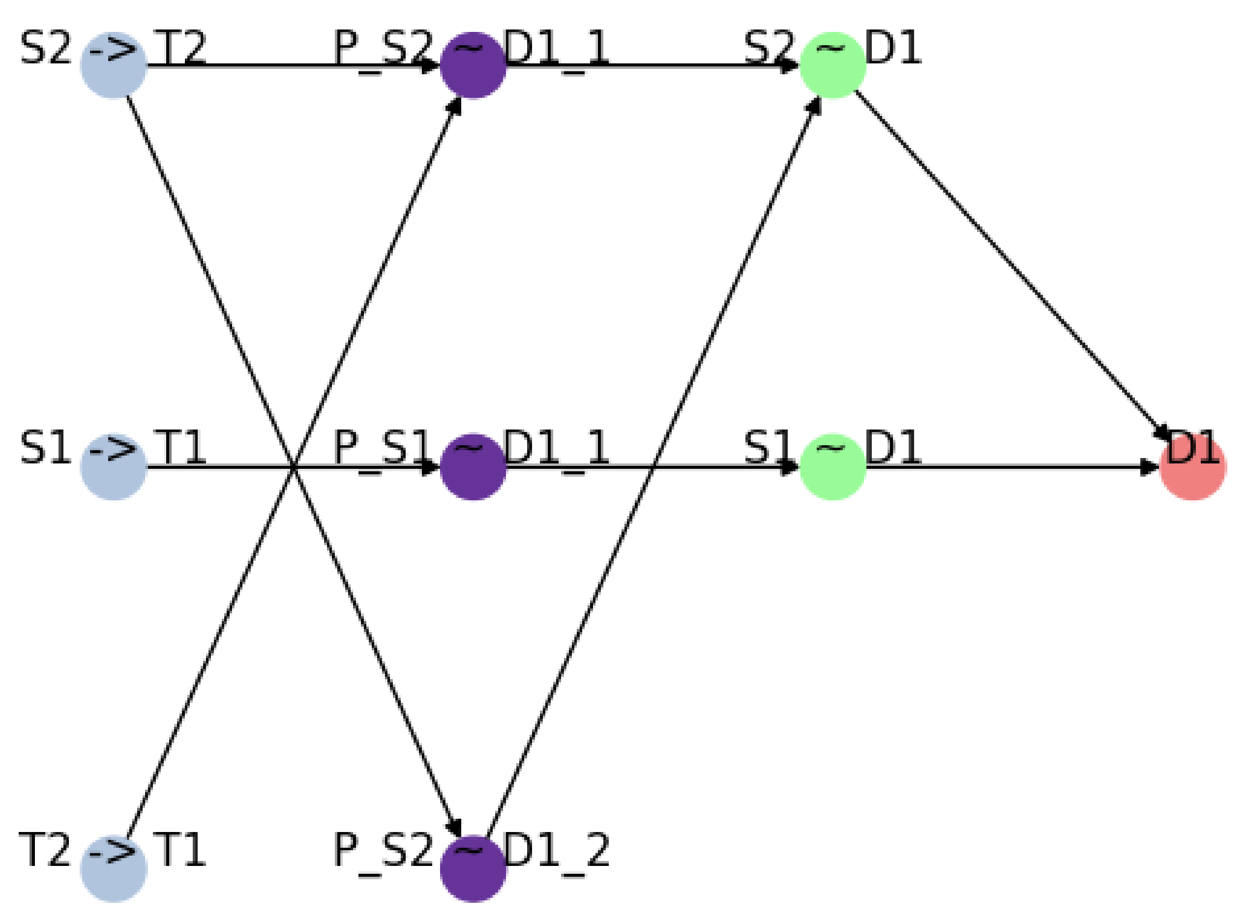
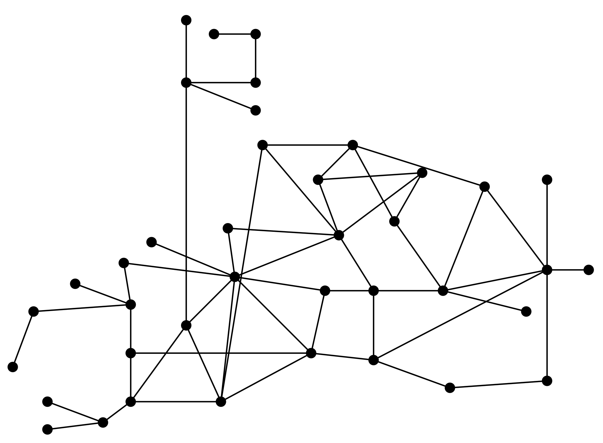
- All paths leading to the relevant demand, whose reliabilities lie on the series multiplication of the actuators’ reliabilties involved in each one, which means the direct product of these probabilities: , implying that all of them must be operative to make the path feasible.In the network example of Figure 1 this is represented with the nodes corresponding to the available paths in the second purple nodes column. The parents for each one are the actuators involved in each path, and they are the same ones whose reliabilities will be multiplied to obtain each path’s one;
- All sources with access to provide the relevant demand. In this case, the reliability for each one is the parallel multiplication of the reliabilities of those paths that provide supply from the relevant source, which means the complementary product of all the complementaries of these probabilities: , implying that one feasible path is enough to make the source available.In the network example of Figure 1, this is represented by the nodes corresponding to the available sources in the third light green nodes column. The parents for each one are the paths supplying from each source, and they are the same ones whose reliabilities will be computed to obtain each source’s one;
- Finally, there is the relevant demand, whose reliability is also a parallel multiplication of the available sources, implying that one available source is enough to provide the supply. In this case, it corresponds to the last column with a single red node of the graph example of Figure 1, and all the sources are the parents to perform the relevant reliability calculation.
3.2. Individual Reliability
“Reliability is determined as the probability that a system (or a component) will perform their functioning satisfactorily for a certain period of time subject to operating conditions.” [13]
3.3. Overall System Reliability Modelling
3.4. Inclusion in the Economic MPC Problem Formulation
3.4.1. Augmented System
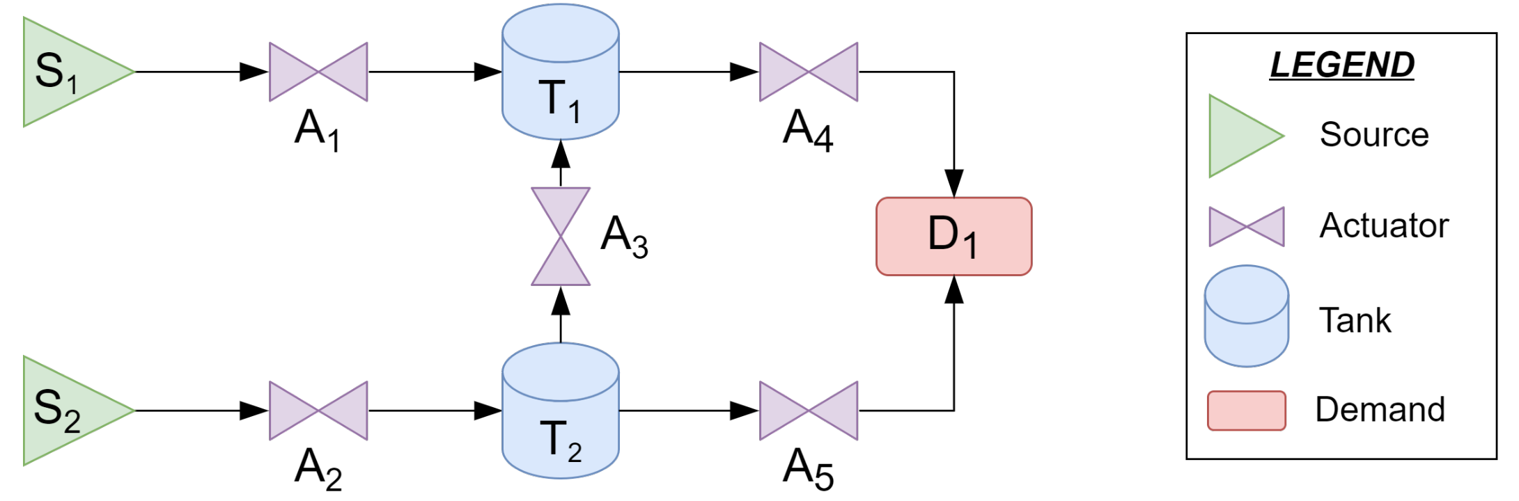
3.4.2. Simple Network Example
3.4.3. Optimization Problem
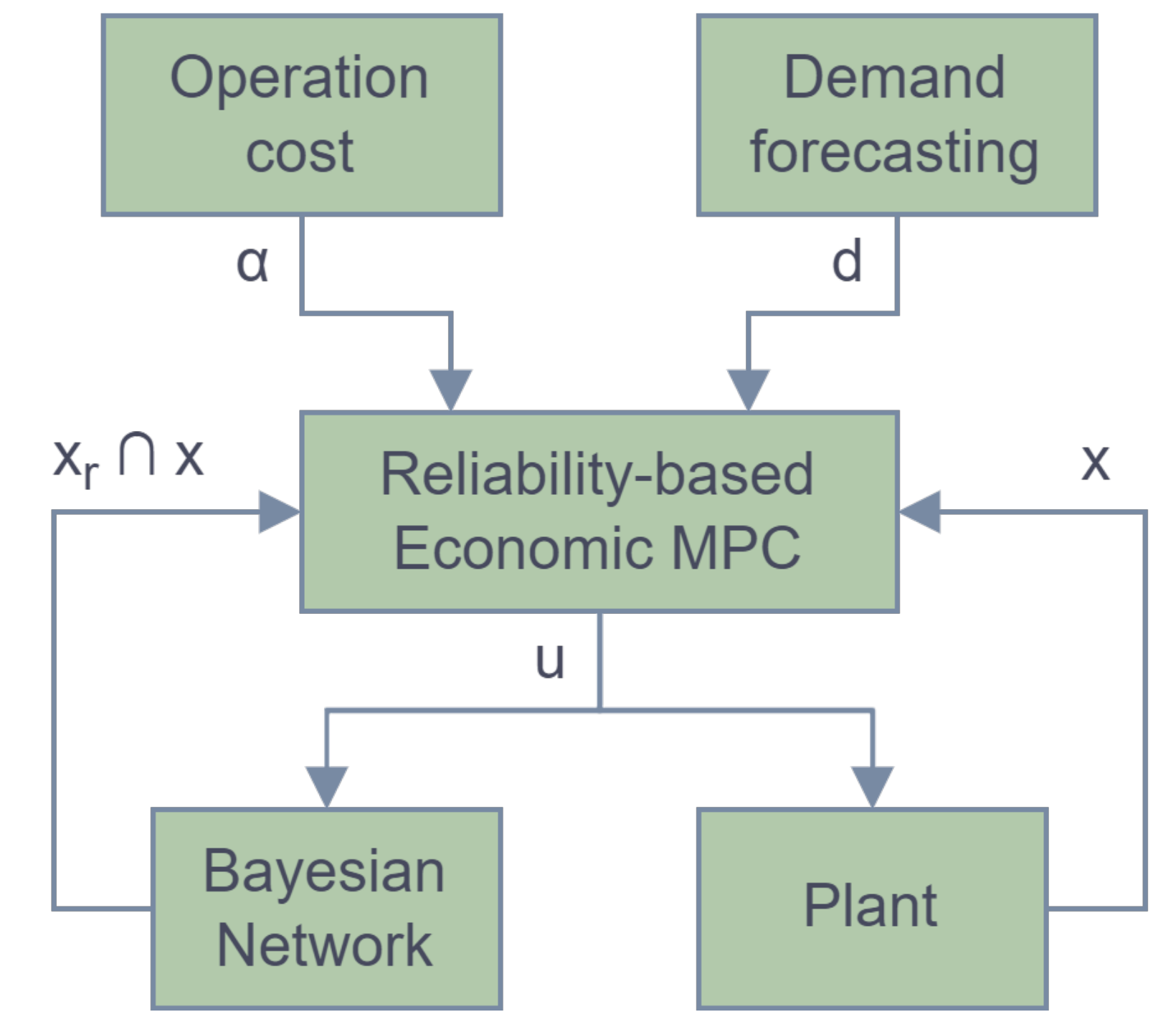
3.4.4. Control Scheme
4. Application
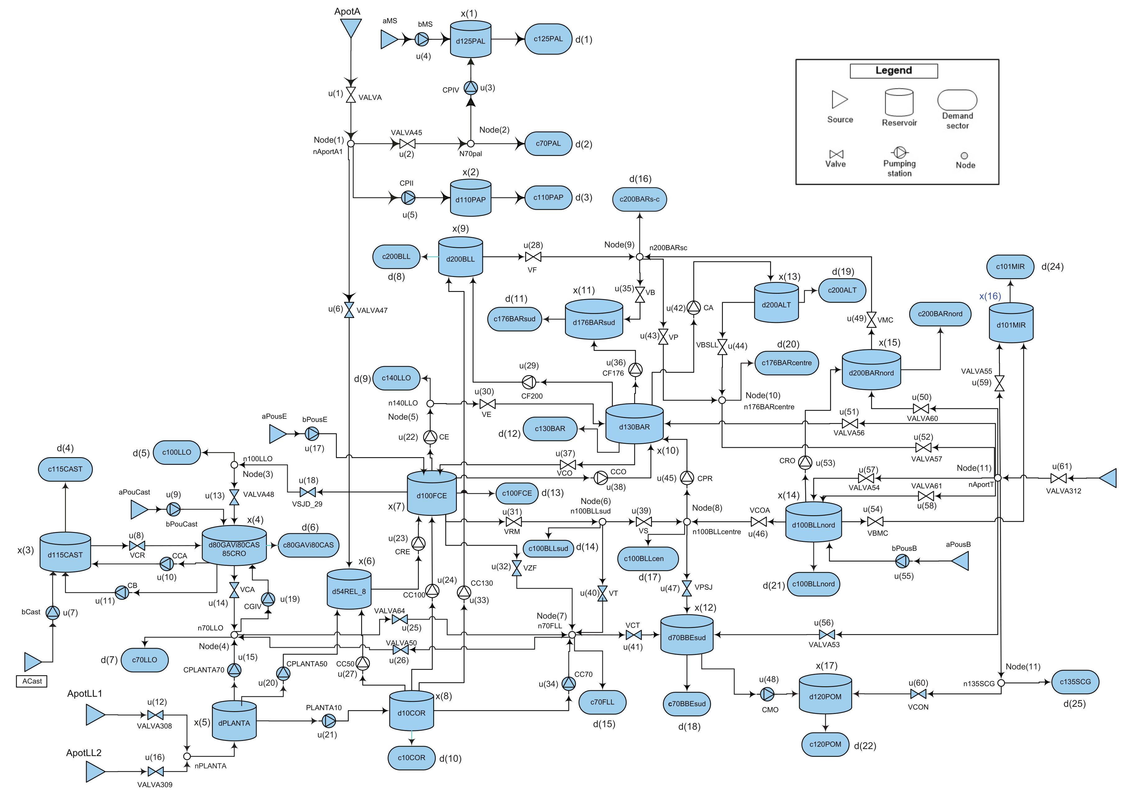
4.1. Case Study
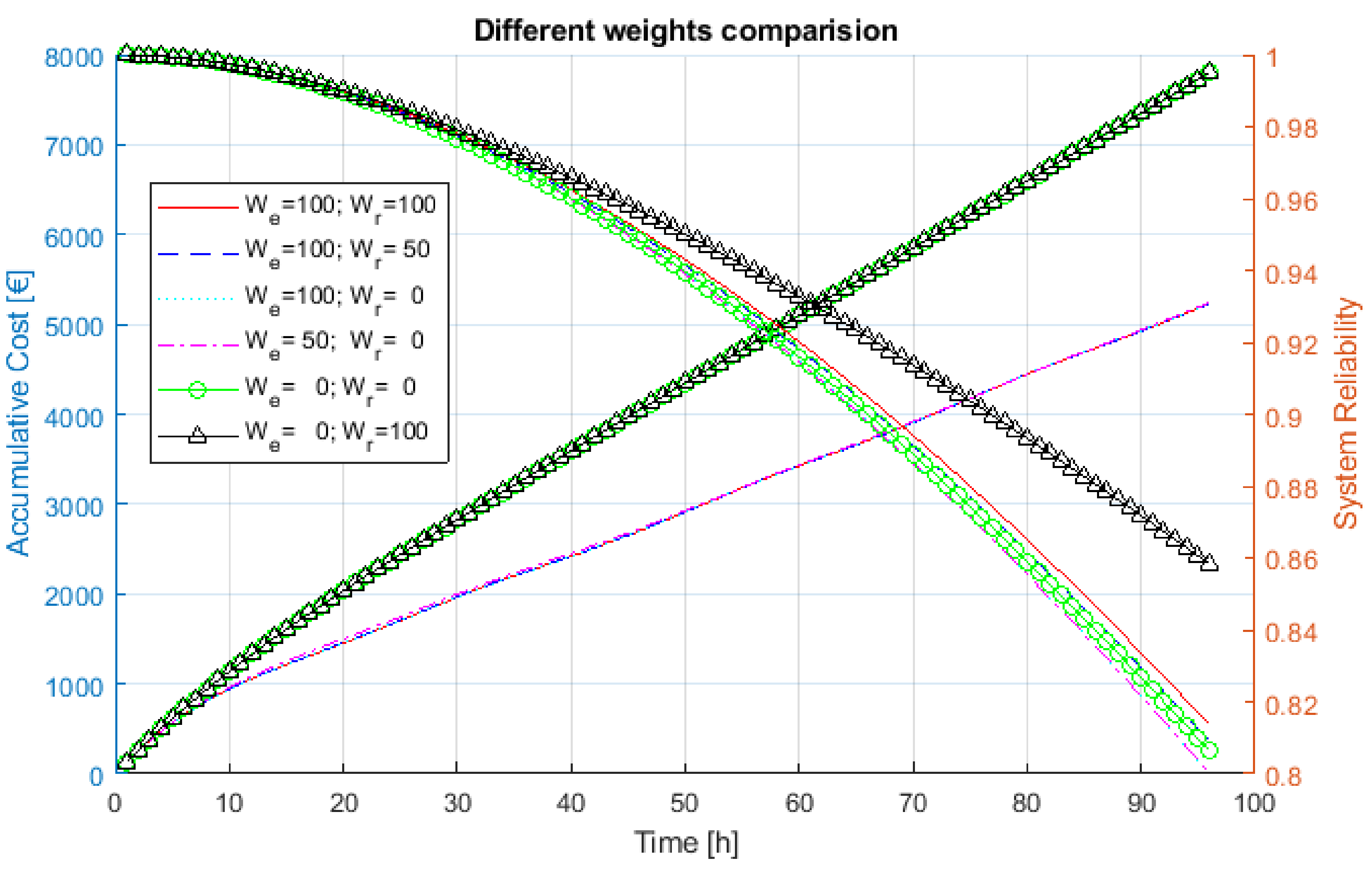
4.2. Results and Discussion
5. Conclusions
Author Contributions
Funding
Institutional Review Board Statement
Informed Consent Statement
Data Availability Statement
Conflicts of Interest
References
- Rawlings, J.B.; Mayne, D.Q. Model Predictive Control: Theory and Design; Nob Hill Pub.: Santa Barbara, CA, USA, 2009. [Google Scholar]
- Karimi Pour, F.; Puig, V.; Ocampo-Martinez, C. Economic Predictive Control of a Pasteurization Plant using a Linear Parameter Varying Model. In Computer Aided Chemical Engineering; Elsevier: Amsterdam, The Netherlands, 2017; Volume 40, pp. 1573–1578. [Google Scholar]
- Karimi, F.; Puig, V.; Cembrano, G. Economic Reliability-Aware MPC-LPV for Operational Management of Flow-Based Water Networks Including Chance-Constraints Programming; Processes: London, UK, 2020. [Google Scholar]
- Grosso, J.M.; Ocampo-Martínez, C.; Puig, V. Reliability-Based Economic Model Predictive Control for Generalised Flow-Based Networks Including Actuators Health-Aware Capabilities; Pearson Education: London, UK, 2016. [Google Scholar]
- Karimi, F.; Puig, V.; Cembrano, G. Economic Health-Aware MPC-LPV Based on DBN Reliability Model for Water Transport Network; Pearson Education: London, UK, 2019. [Google Scholar]
- Gokdere, L.; Chiu, S.L.; Keller, K.J.; Vian, J. Lifetime control of electromechanical actuators. In Proceedings of the 2005 IEEE Aerospace Conference, Big Sky, MT, USA, 5–12 March 2005; pp. 3523–3531. [Google Scholar]
- Pereira, E.B.; Galvao, R.K.H.; Yoneyama, T. Model predictive control using prognosis and health monitoring of actuators. In Proceedings of the 2010 IEEE International Symposium on Industrial Electronics (ISIE), Bari, Italy, 4–7 July 2010; pp. 237–243. [Google Scholar]
- Salazar, J.C.; Weber, P.; Sarrate, R.; Theilliol, D.; Nejjari, F. MPC design based on a DBN reliability model: Application to drinking water networks. IFAC-PapersOnLine 2015, 48, 688–693. [Google Scholar] [CrossRef]
- Karimi Pour, F.; Puig, V.; Cembrano, G. Health-aware LPV-MPC based on system reliability assessment for drinking water networks. In Proceedings of the 2nd IEEE Conference on Control Technology and Applications, Copenhagen, Denmark, 21–24 August 2018. [Google Scholar]
- Grosso, J.M.; Ocampo-Martínez, C.; Puig, V. A service reliability model predictive control with dynamic safety stocks and actuators health monitoring for drinking water networks. In Proceedings of the 2012 IEEE 51st Annual Conference on Decision and Control (CDC), Maui, HI, USA, 10–13 December 2012; pp. 4568–4573. [Google Scholar]
- Maciejowski, J.M. Predictive Control: With Constraints; Pearson Education: London, UK, 2002. [Google Scholar]
- Jiang, R.; Jardine, A.K. Health state evaluation of an item: A general framework and graphical representation. Reliab. Eng. Syst. Saf. 2008, 93, 89–99. [Google Scholar] [CrossRef]
- Gertsbakh, I. Reliability Theory: With Applications to Preventive Maintenance; Springer: Berlin/Heidelberg, Germany, 2013. [Google Scholar]
- Baecher, G.B.; Christian, J.T. Reliability and Statistics in Geotechnical Engineering; John Wiley & Sons: Hoboken, NJ, USA, 2005. [Google Scholar]
- Ocampo-Martínez, C.; Puig, V.; Cembrano, G.; Creus, R.; Minoves, M. Improving water management efficiency by using optimization-based control strategies: The Barcelona case study. Water Sci. Technol. Water Supply 2009, 9, 565–575. [Google Scholar] [CrossRef]


| R | Bayesian Networks | Classical Reliability | Proposed Approach |
| 0.9 | 0.99 | 0.9981 | 0.9981 |
| 0.8 | 0.96 | 0.9856 | 0.9856 |
| 0.6 | 0.84 | 0.8976 | 0.8976 |
Publisher’s Note: MDPI stays neutral with regard to jurisdictional claims in published maps and institutional affiliations. |
© 2022 by the authors. Licensee MDPI, Basel, Switzerland. This article is an open access article distributed under the terms and conditions of the Creative Commons Attribution (CC BY) license (https://creativecommons.org/licenses/by/4.0/).
Share and Cite
Pedrosa, J.; Puig, V.; Nejjari, F. Health-Aware Economic MPC for Operational Management of Flow-Based Networks Using Bayesian Networks. Water 2022, 14, 1538. https://doi.org/10.3390/w14101538
Pedrosa J, Puig V, Nejjari F. Health-Aware Economic MPC for Operational Management of Flow-Based Networks Using Bayesian Networks. Water. 2022; 14(10):1538. https://doi.org/10.3390/w14101538
Chicago/Turabian StylePedrosa, Javier, Vicenç Puig, and Fatiha Nejjari. 2022. "Health-Aware Economic MPC for Operational Management of Flow-Based Networks Using Bayesian Networks" Water 14, no. 10: 1538. https://doi.org/10.3390/w14101538
APA StylePedrosa, J., Puig, V., & Nejjari, F. (2022). Health-Aware Economic MPC for Operational Management of Flow-Based Networks Using Bayesian Networks. Water, 14(10), 1538. https://doi.org/10.3390/w14101538