
Automated Extraction of Lake Water Bodies in Complex Geographical Environments by Fusing Sentinel-1/2 Data


Abstract
:1. Introduction

| Methods | Subcategories | Literature | Characteristics |
|---|---|---|---|
| Only optical | Single-band | Work et al., 1976 [8] | This method is simple to calculate, but it is easily affected by shadows of mountains and buildings, and it is difficult to determine an optimal threshold. |
| Two-band | Xu et al., 2006 [12] | ||
| Multi-band | Feyisa et al., 2014 [14] | ||
| Only SAR | Single-polarized | Guo et al., 1999 [23] | This method can reduce misclassification caused by the spectral heterogeneity, but it is easily affected by mountains and smooth-material ground objects. |
| Dual-polarized | Tian et al., 2017 [19] | ||
| Quad-polarized | Guo et al., 1997 [24] | ||
| Data fusion | SAR-optical data | Saghafi et al., 2021 [22] | This method can suppress the interference of shadows, water quality, and smooth-material ground objects. |
2. Materials and Methods
2.1. Materials
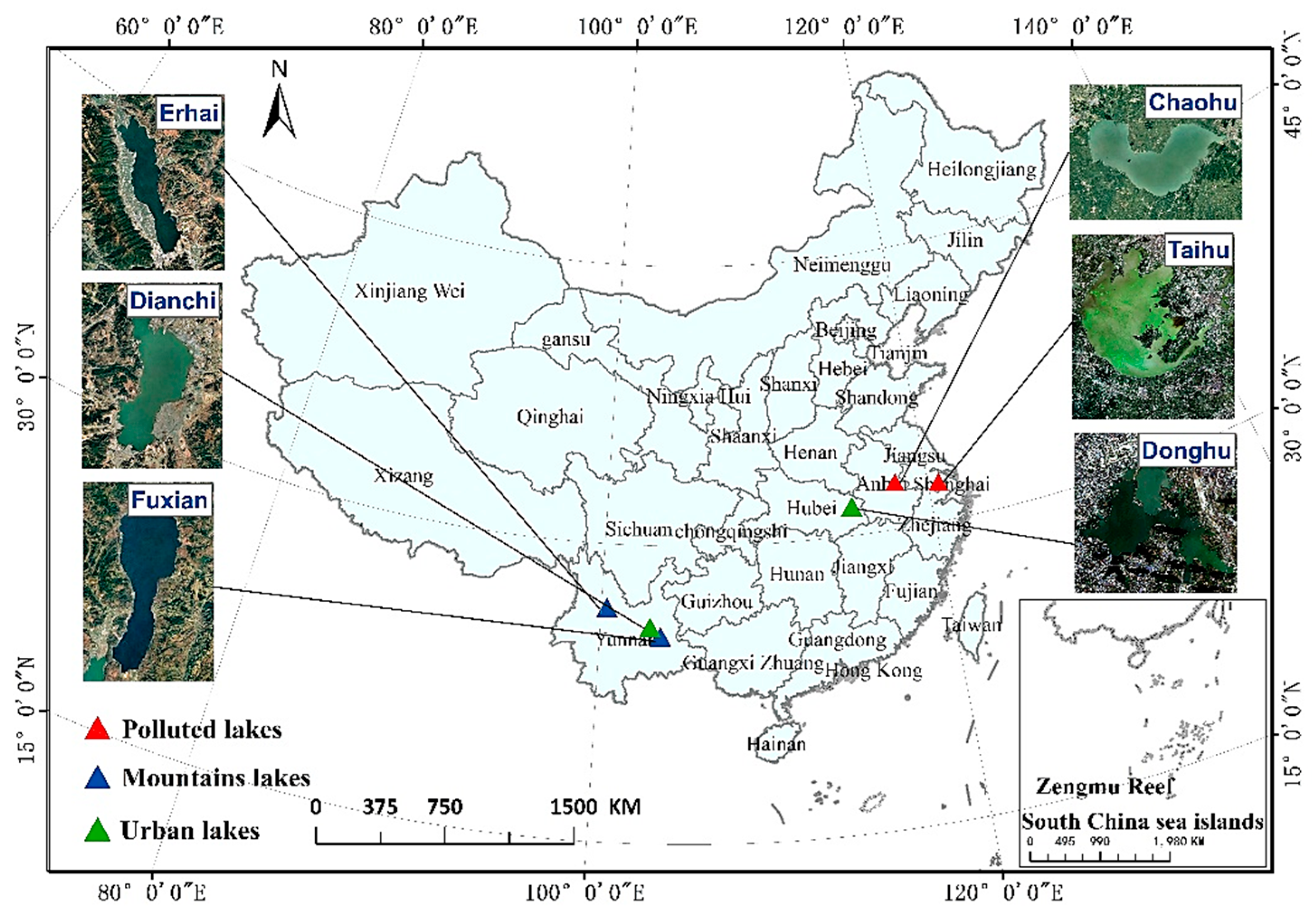
2.1.1. Study Area
2.1.2. Data
| Satellite | Senor Type | Spatial Resolution (m) | Number of Channels | Acquisition Data |
|---|---|---|---|---|
| Sentinel-1 | Optical | 10 | 2 | November–December 2019 |
| Sentinel-2 | RADAR | 10, 20, and 60 | 13 | November–December 2019 |
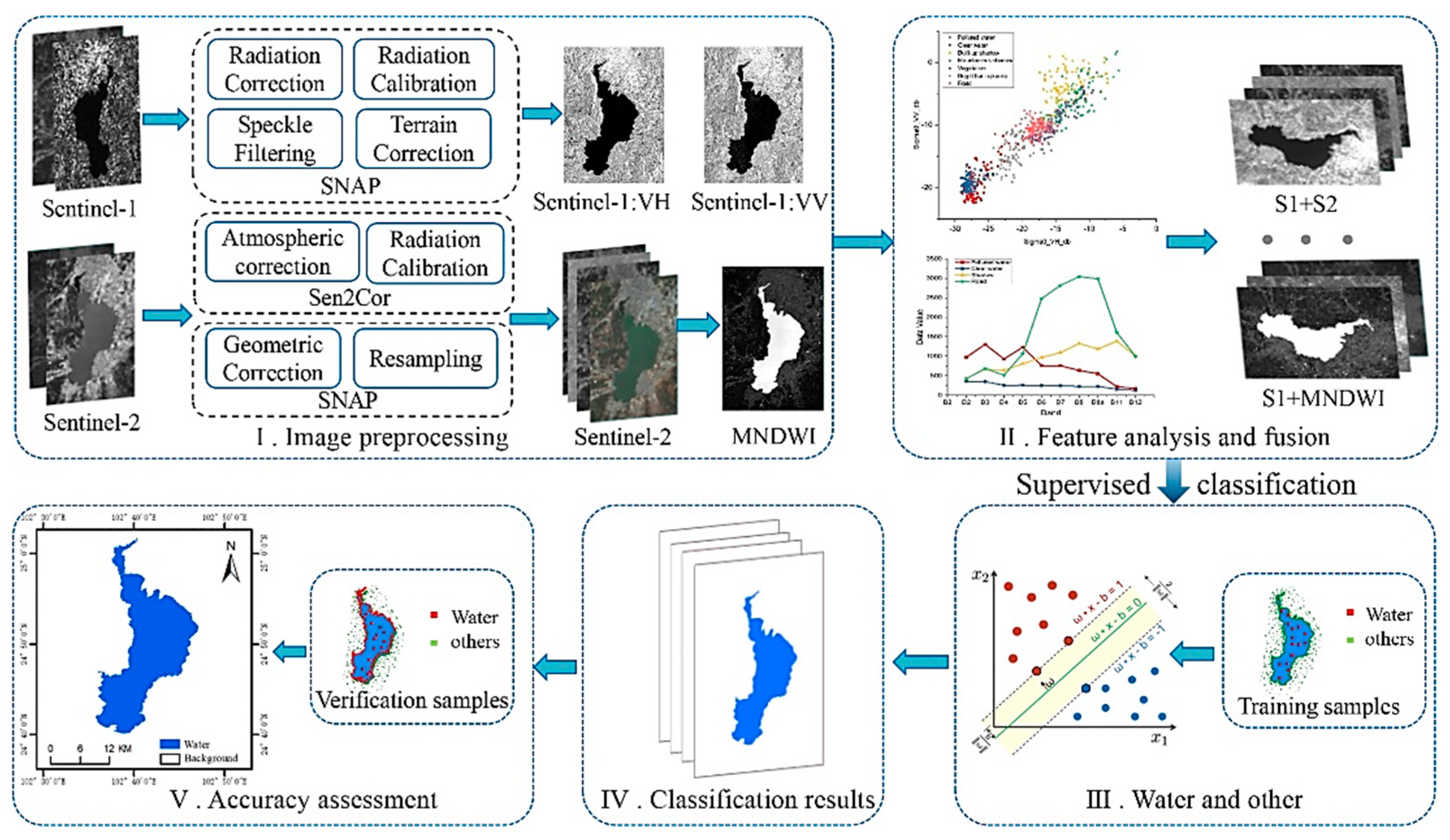
2.2. Methods
2.2.1. Dataset Preprocessing
2.2.2. Water Index
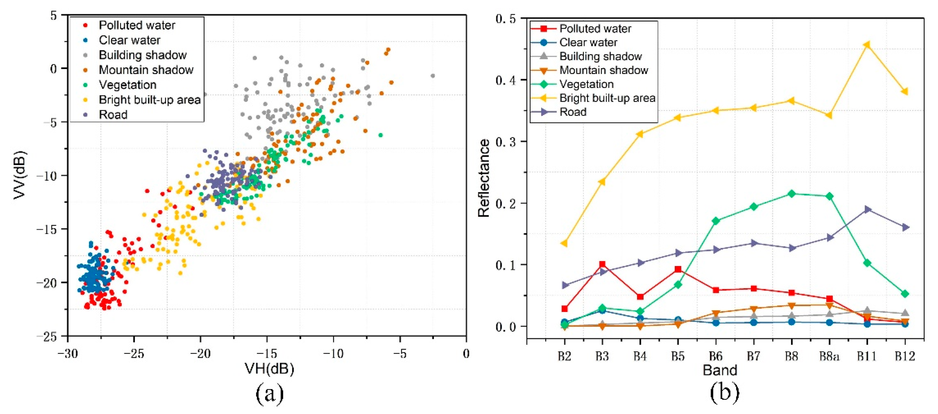
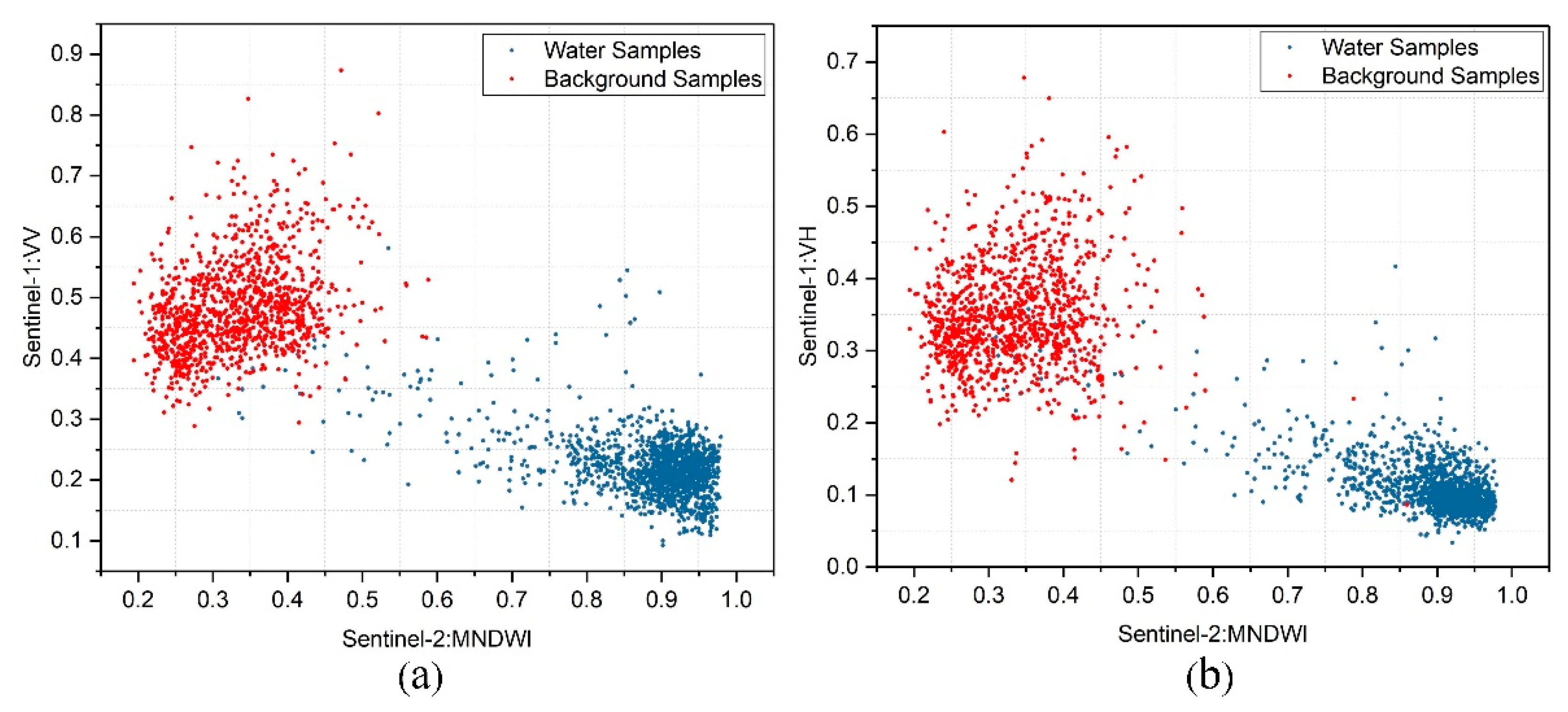
2.2.3. Features Analysis for LWB Extraction
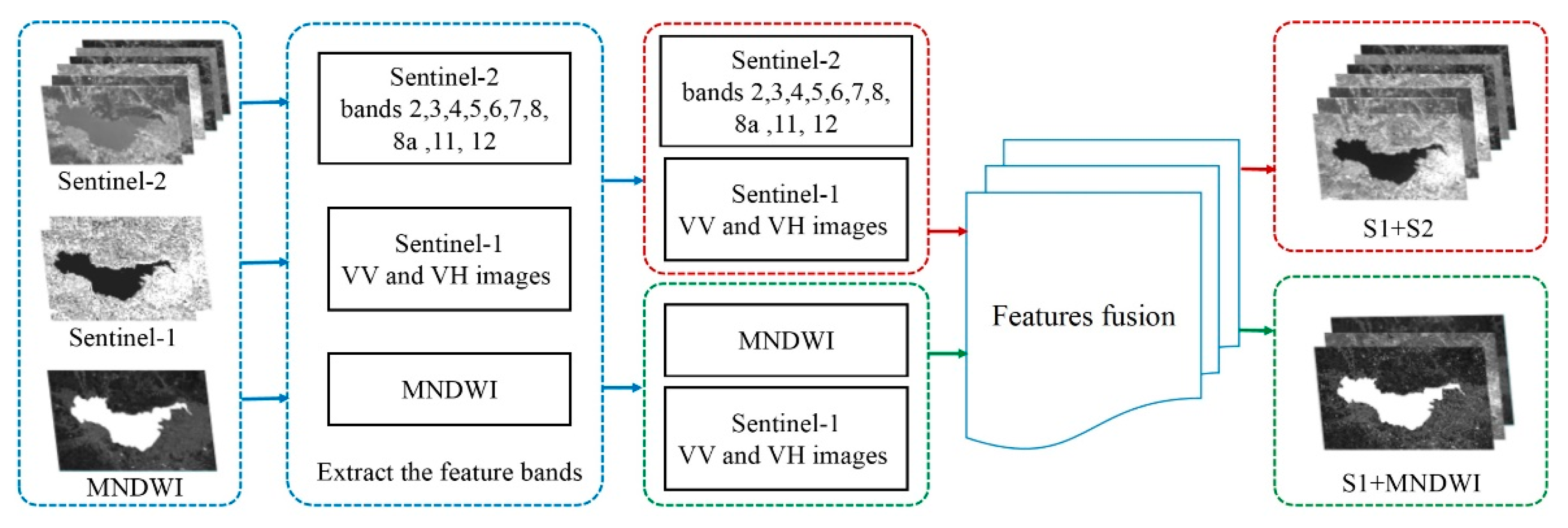
2.2.4. Feature Fusion for LWB Extraction
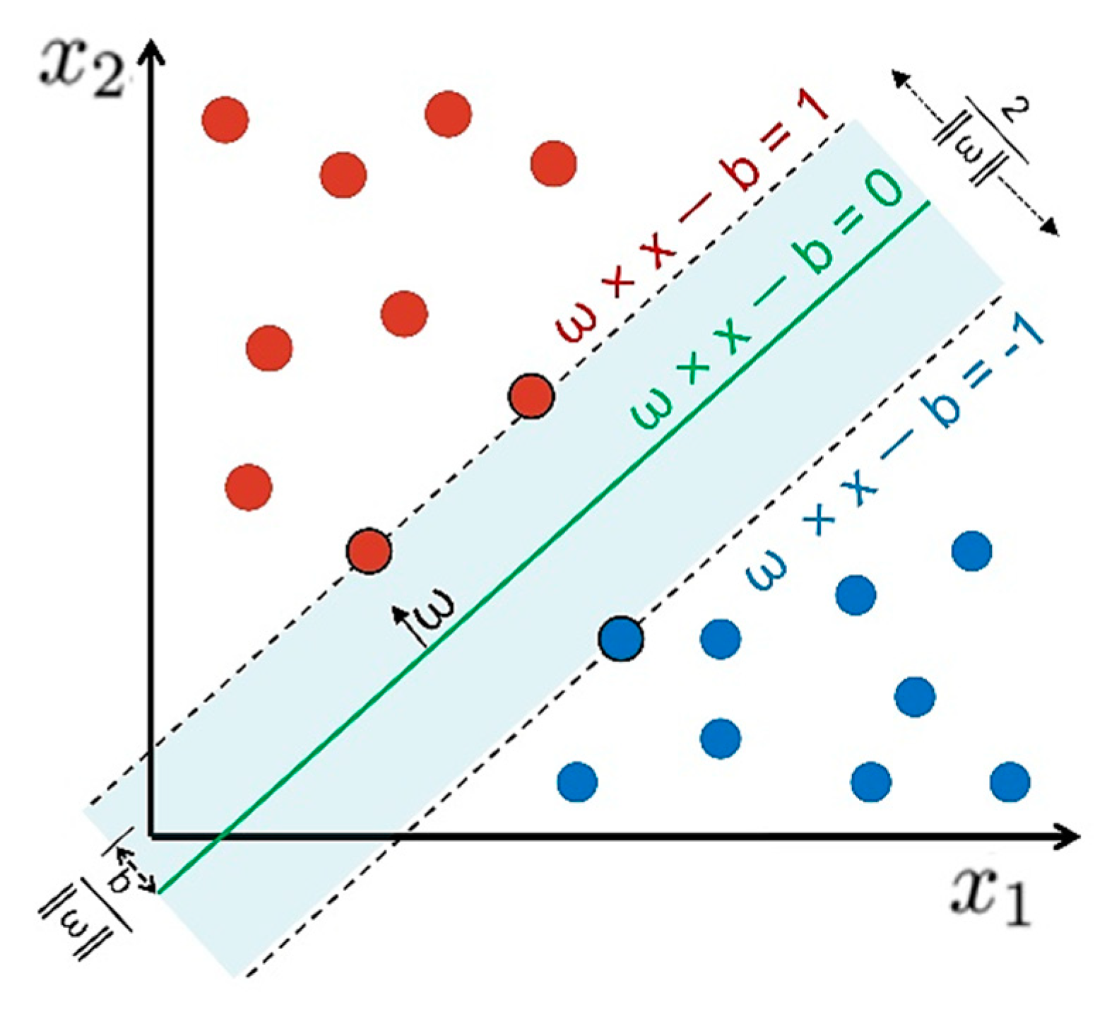
2.2.5. Classification Method
2.2.6. Accuracy Assessment
2.2.7. Experiment Design
3. Results
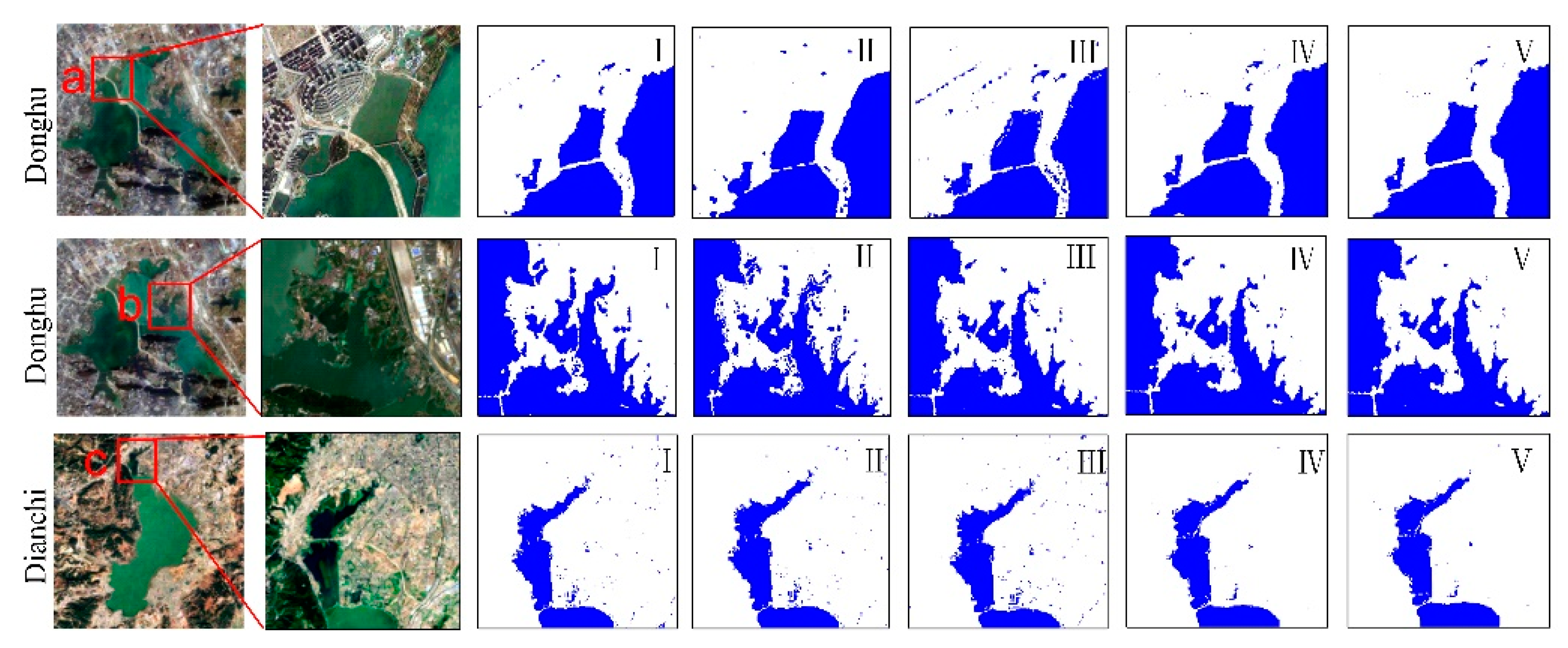
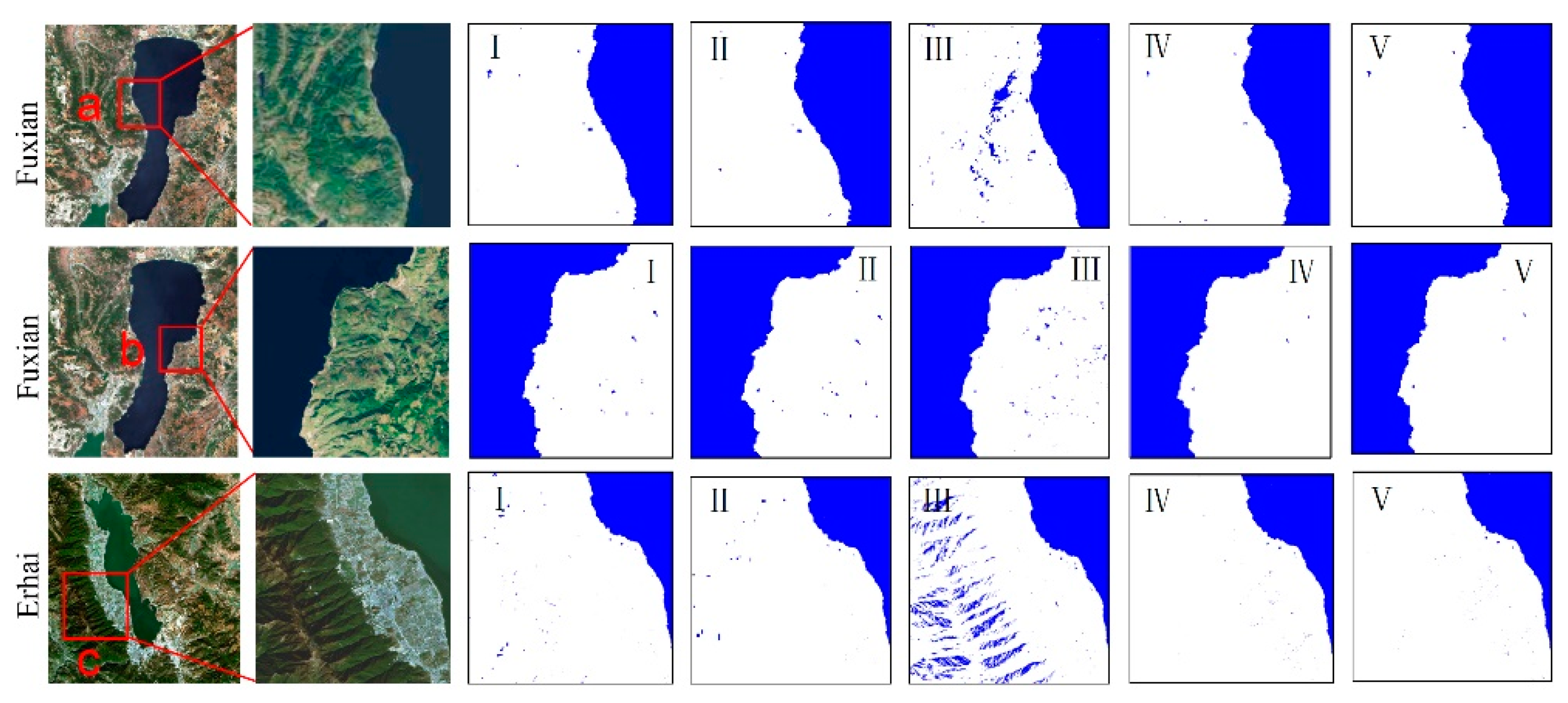
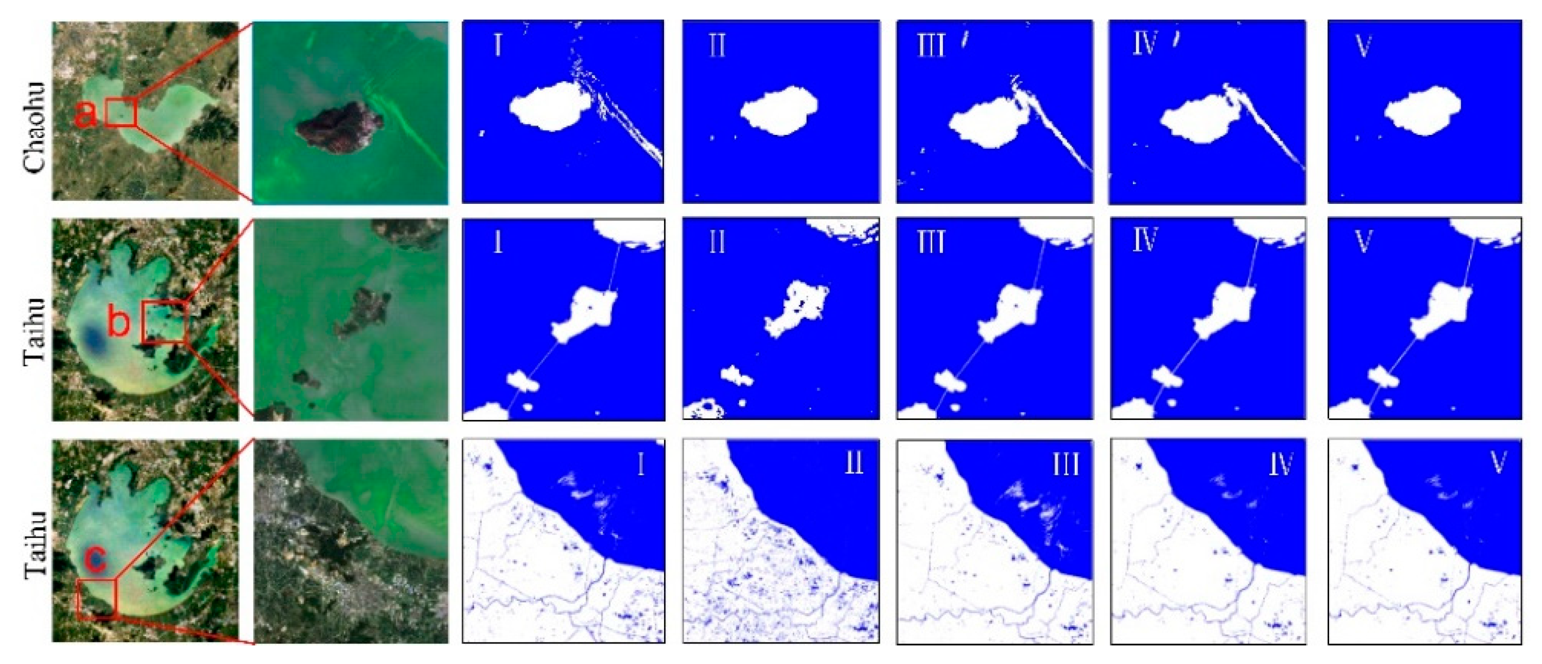
3.1. LWB Extraction Performance
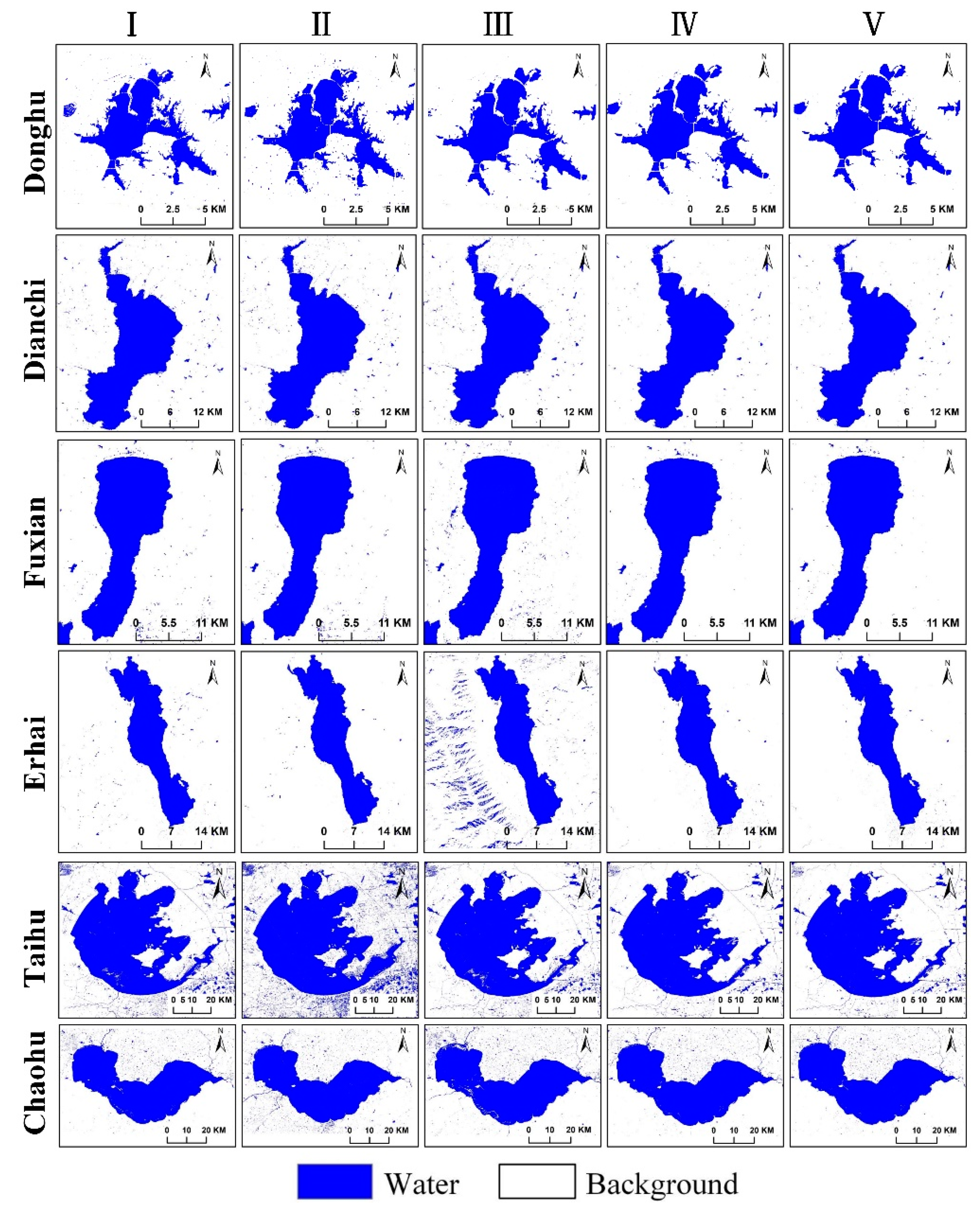
3.2. Accuracy Assessment
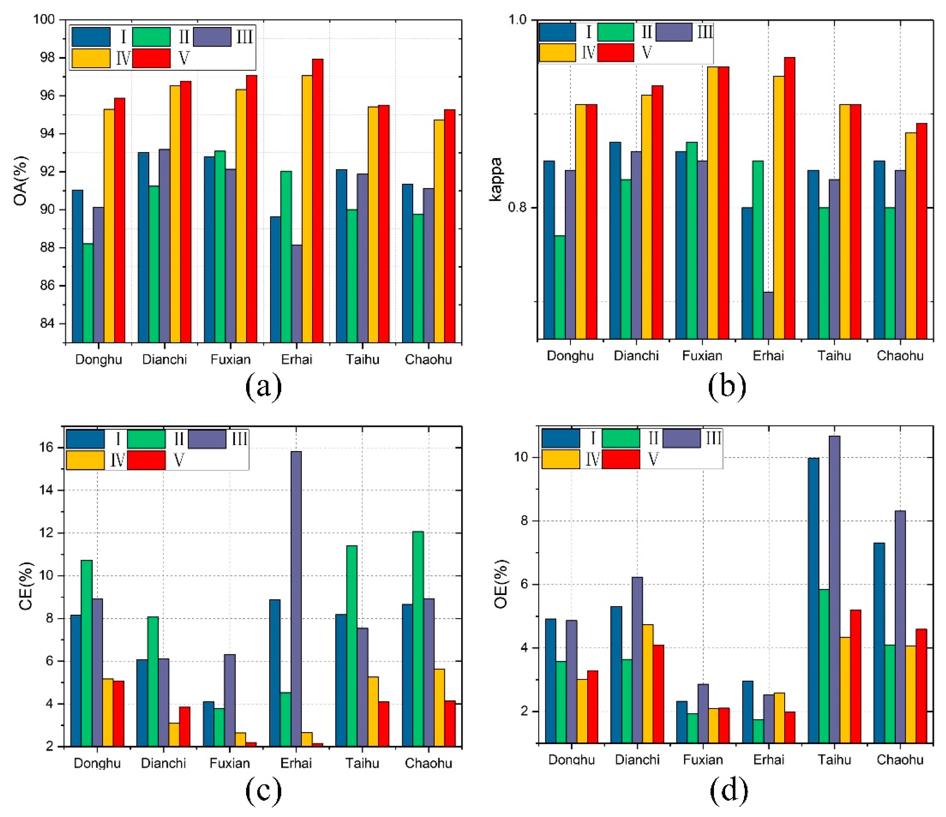
| Scheme | Donghu | Dianchi | Fuxian | Erhai | Taihu | Chaohu | ||||||
|---|---|---|---|---|---|---|---|---|---|---|---|---|
| OA% | Kappa | OA% | Kappa | OA% | Kappa | OA% | Kappa | OA% | Kappa | OA% | Kappa | |
| I | 91.04 | 0.85 | 93.01 | 0.87 | 92.79 | 0.86 | 89.63 | 0.80 | 92.11 | 0.84 | 91.35 | 0.85 |
| II | 88.21 | 0.77 | 91.24 | 0.83 | 93.08 | 0.87 | 92.04 | 0.85 | 90.01 | 0.80 | 89.76 | 0.80 |
| III | 90.13 | 0.84 | 93.17 | 0.86 | 92.13 | 0.85 | 88.15 | 0.71 | 91.87 | 0.83 | 91.11 | 0.84 |
| IV | 95.29 | 0.91 | 96.53 | 0.92 | 96.32 | 0.95 | 97.06 | 0.94 | 95.42 | 0.91 | 94.72 | 0.88 |
| V | 95.87 | 0.91 | 96.77 | 0.93 | 97.07 | 0.95 | 97.93 | 0.96 | 95.51 | 0.91 | 95.28 | 0.89 |
| Scheme | Donghu | Dianchi | Fuxian | Erhai | Taihu | Chaohu | ||||||
|---|---|---|---|---|---|---|---|---|---|---|---|---|
| CE% | OE% | CE% | OE% | CE% | OE% | CE% | OE% | CE% | OE% | CE% | OE% | |
| I | 8.15 | 4.91 | 6.07 | 5.31 | 4.09 | 2.32 | 8.87 | 2.96 | 8.18 | 9.98 | 8.66 | 7.31 |
| II | 10.73 | 3.57 | 8.08 | 3.64 | 3.78 | 1.94 | 4.53 | 1.74 | 11.41 | 5.84 | 12.07 | 4.10 |
| III | 8.92 | 4.86 | 6.10 | 6.23 | 6.31 | 2.86 | 15.81 | 2.52 | 7.54 | 10.67 | 8.93 | 8.31 |
| IV | 5.17 | 3.02 | 3.09 | 4.73 | 2.64 | 2.09 | 2.65 | 2.59 | 5.26 | 4.34 | 5.63 | 4.07 |
| V | 5.08 | 3.29 | 3.85 | 4.09 | 2.19 | 2.11 | 2.15 | 1.98 | 4.09 | 5.19 | 4.14 | 4.59 |
4. Discussion
4.1. Lake Environmental Noise
4.2. Lake Water Body Types
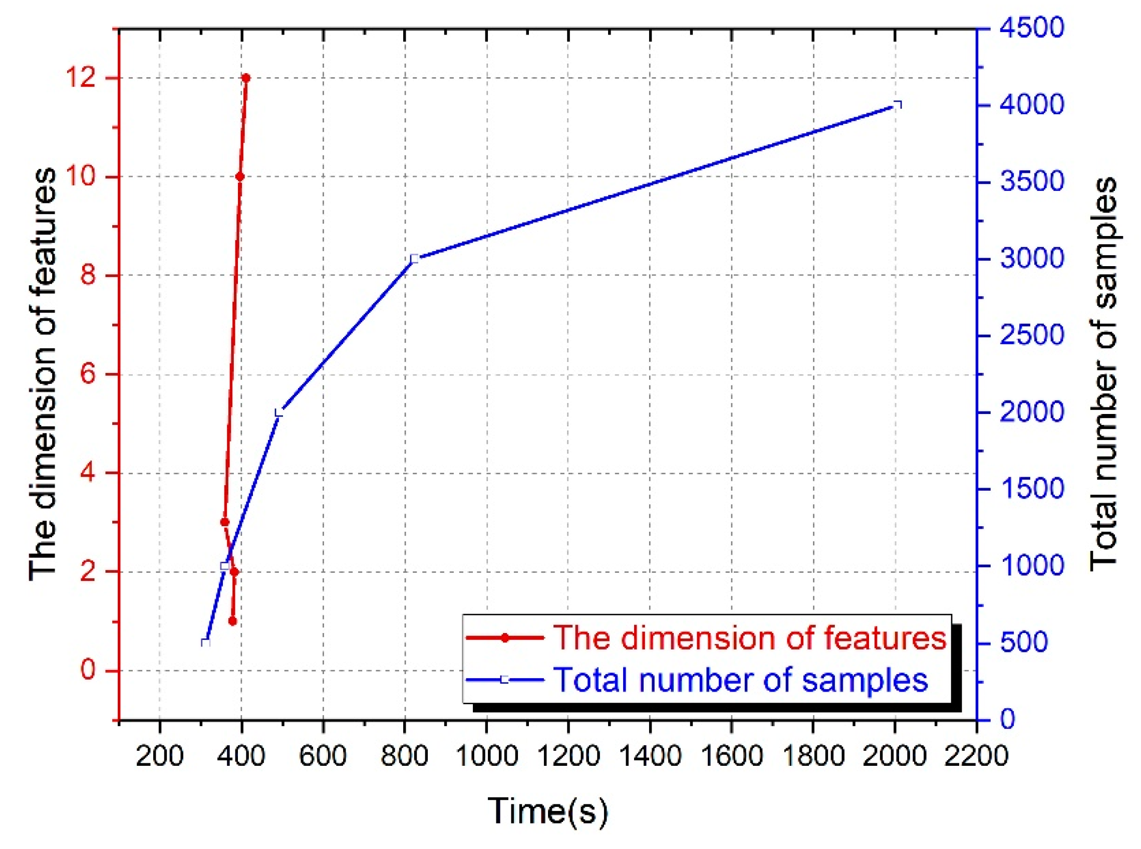
4.3. Computational Complexity
5. Conclusions
Author Contributions
Funding
Institutional Review Board Statement
Informed Consent Statement
Data Availability Statement
Conflicts of Interest
Appendix A
| Acronyms | Full Name |
|---|---|
| LWB | Lake water body |
| LSWB | Land surface water body |
| SAR | Synthetic aperture radar |
| S1 | Sentinel-1 |
| S2 | Sentinel-2 |
| SVM | Support vector machine |
References
- Huang, L.; Xu, X.; Zhai, J.; Sun, C. Local background climate determining the dynamics of plateau lakes in China. Reg. Environ. Chang. 2016, 16, 2457–2470. [Google Scholar] [CrossRef]
- Wu, P.; Shen, H.; Cai, N.; Zeng, C.; Wu, Y.; Wang, B. Spatiotemporal analysis of water area annual variations using a Landsat time series: A case study of nine plateau lakes in Yunnan province, China. Int. J. Remote Sens. 2016, 37, 5826–5842. [Google Scholar] [CrossRef]
- Wang, Z.; Gao, X.; Zhang, Y.; Zhao, G. MSLWENet: A Novel Deep Learning Network for Lake Water Body Extraction of Google Remote Sensing Images. Remote Sens. 2020, 12, 4140. [Google Scholar] [CrossRef]
- Xu, Y.; Liu, W.; Song, J.; Yao, L.; Gu, S. Dynamic Monitoring of the Lake Area in the Middle and Lower Reaches of the Yangtze River Using MODIS Images Between 2000 and 2016. IEEE J. Sel. Top. Appl. Earth Obs. Remote Sens. 2018, 11, 4690–4700. [Google Scholar] [CrossRef]
- Jiang, H.; Feng, M.; Zhu, Y.; Lu, N.; Huang, J.; Xiao, T. An Automated Method for Extracting Rivers and Lakes from Landsat Imagery. Remote Sens. 2014, 6, 5067–5089. [Google Scholar] [CrossRef] [Green Version]
- Du, Y.; Zhang, Y.; Ling, F.; Wang, Q.; Li, W.; Li, X. Water Bodies’ Mapping from Sentinel-2 Imagery with Modified Normalized Difference Water Index at 10-m Spatial Resolution Produced by Sharpening the SWIR Band. Remote Sens. 2016, 8, 354. [Google Scholar] [CrossRef] [Green Version]
- Zhang, G.; Zheng, G.; Gao, Y.; Xiang, Y.; Lei, Y.; Li, J. Automated Water Classification in the Tibetan Plateau Using Chinese GF-1 WFV Data. Photogramm. Eng. Remote Sens. 2017, 83, 509–519. [Google Scholar] [CrossRef]
- Work, E.; Gilmer, D.S. Utilization of satellite data for inventorying prairie ponds and lakes. Photogramm. Eng. Remote Sens. 1976, 42, 685–694. [Google Scholar]
- McFeeters, S.K. The use of the Normalized Difference Water Index (NDWI) in the delineation of open water features. Int. J. Remote Sens. 1996, 17, 1425–1432. [Google Scholar] [CrossRef]
- Yang, X.; Qin, Q.; Grussenmeyer, P.; Koehl, M. Urban surface water body detection with suppressed built-up noise based on water indices from Sentinel-2 MSI imagery. Remote Sens. Environ. 2018, 219, 259–270. [Google Scholar] [CrossRef]
- Li, W.; Du, Z.; Ling, F.; Zhou, D.; Wang, H.; Gui, Y. A Comparison of Land Surface Water Mapping Using the Normalized Difference Water Index from TM, ETM+ and ALI. Remote Sens. 2013, 5, 5530–5549. [Google Scholar] [CrossRef] [Green Version]
- Xu, H. Modification of normalised difference water index (NDWI) to enhance open water features in remotely sensed imagery. Int. J. Remote Sens. 2006, 27, 3025–3033. [Google Scholar] [CrossRef]
- Li, L.; Su, H.; Du, Q.; Wu, T. A novel surface water index using local background information for long term and large-scale Landsat images. ISPRS J. Photogramm. Remote Sens. 2021, 172, 59–78. [Google Scholar] [CrossRef]
- Feyisa, G.L.; Meilby, H.; Fensholt, R.; Proud, S.R. Automated Water Extraction Index: A new technique for surface water mapping using Landsat imagery. Remote Sens. Environ. 2014, 140, 23–35. [Google Scholar] [CrossRef]
- Wang, X.; Xie, S.; Zhang, X.; Chen, C.; Guo, H.; Du, J. A robust Multi-Band Water Index (MBWI) for automated extraction of surface water from Landsat 8 OLI imagery. Int. J. Appl. Earth Obs. Geoinf. 2018, 68, 73–91. [Google Scholar] [CrossRef]
- Ciuonzo, D.; Carotenuto, V.; De Maio, A. On multiple covariance equality testing with application to SAR change detection. IEEE Trans. Signal Process. 2017, 65, 5078–5091. [Google Scholar] [CrossRef]
- Saha, S.; Bovolo, F.; Bruzzone, L. Building change detection in VHR SAR images via unsupervised deep transcoding. IEEE Trans. Geosci. Remote Sens. 2020, 59, 1917–1929. [Google Scholar] [CrossRef]
- Wang, Z.L.; Liao, M.S.; Zhang, L. Detecting and characterizing deformations of the left bank slope near the Jinping hydropower station with time series Sentinel-1 data. Remote Sens. Land Resour. 2019, 31, 204–209. [Google Scholar]
- Tian, H.; Li, W.; Wu, M.; Huang, N.; Li, G.; Li, X. Dynamic Monitoring of the Largest Freshwater Lake in China Using a New Water Index Derived from High Spatiotemporal Resolution Sentinel-1A Data. Remote Sens. 2017, 9, 521. [Google Scholar] [CrossRef] [Green Version]
- Zhang, Y.; Zhang, G.; Zhu, T. Seasonal cycles of lakes on the Tibetan Plateau detected by Sentinel-1 SAR data. Sci. Total Environ. 2019, 703, 135563. [Google Scholar] [CrossRef]
- Valdiviezo-Navarro, J.C.; Salazar-Garibay, A.; Téllez-Quiñones, A.; Orozco-del-Castillo, M.; López-Caloca, A.A. Inland water body extraction in complex reliefs from Sentinel-1 satellite data. J. Appl. Remote Sens. 2019, 13, 016524. [Google Scholar] [CrossRef]
- Saghafi, M.; Ahmadi, A.; Bigdeli, B. Sentinel-1 and Sentinel-2 data fusion system for surface water extraction. J. Appl. Remote Sens. 2021, 15, 014521. [Google Scholar] [CrossRef]
- Guo, H.D. Analysis of Radar Remote Sensing Imagery in China; Science Press: Beijing, China, 1999. [Google Scholar]
- Guo, H.D. Spaceborne Multifrequency, Polarametric and Interferometric Radar for Detection of the Targets on Earth Surface and Subsurface. J. Remote Sens. 1997, 1, 32–39. [Google Scholar]
- Bioresita, F.; Puissant, A.; Stumpf, A.; Malet, J.-P. Fusion of Sentinel-1 and Sentinel-2 image time series for permanent and temporary surface water mapping. Int. J. Remote Sens. 2019, 40, 9026–9049. [Google Scholar] [CrossRef]
- Slinski, K.M.; Hogue, T.S.; McCray, J.E. Active-Passive Surface Water Classification: A New Method for High-Resolution Monitoring of Surface Water Dynamics. Geophys. Res. Lett. 2019, 46, 4694–4704. [Google Scholar] [CrossRef]
- Schmitt, M. Potential of Large-Scale Inland Water Body Mapping from Sentinel-1/2 Data on the Example of Bavaria’s Lakes and Rivers. PFG J. Photogramm. Remote Sens. Geoinf. Sci. 2020, 88, 271–289. [Google Scholar] [CrossRef]
- Mahdianpari, M.; Salehi, B.; Mohammadimanesh, F.; Homayouni, S.; Gill, E. The first wetland inventory map of newfoundland at a spatial resolution of 10 m using sentinel-1 and sentinel-2 data on the google earth engine cloud computing platform. Remote Sens. 2019, 11, 43. [Google Scholar] [CrossRef] [Green Version]
- Poortinga, A.; Tenneson, K.; Shapiro, A.; Nquyen, Q.; San Aung, K.; Chishtie, F. Mapping plantations in Myanmar by fusing landsat-8, sentinel-2 and sentinel-1 data along with systematic error quantification. Remote Sens. 2019, 11, 831. [Google Scholar] [CrossRef] [Green Version]
- Li, C.; Shao, Z.; Zhang, L.; Huang, X.; Zhang, M. A comparative analysis of index-based methods for impervious surface extraction using multi-seasonal Sentinel-2 satellite data. IEEE J. Sel. Top. Appl. Earth Obs. Remote Sens. 2021, 14, 3682–3694. [Google Scholar] [CrossRef]
- Tavares, P.A.; Beltrão, N.E.S.; Guimarães, U.S.; Teodoro, A.C. Integration of Sentinel-1 and Sentinel-2 for Classification and LULC Mapping in the Urban Area of Belém, Eastern Brazilian Amazon. Sensors 2019, 19, 1140. [Google Scholar] [CrossRef] [Green Version]
- Liangpei, Z.; Xin, H.; Bo, H.; Pingxiang, L. A pixel shape index coupled with spectral information for classification of high spatial resolution remotely sensed imagery. IEEE Trans. Geosci. Remote Sens. 2006, 44, 2950–2961. [Google Scholar] [CrossRef]
- Liu, Z.; Blasch, E.; Bhatnagar, G.; John, V.; Wu, W.; Blum, R.S. Fusing synergistic information from multi-sensor images: An overview from implementation to performance assessment. Inf. Fusion 2018, 42, 127–145. [Google Scholar] [CrossRef]
- Cortes, C.; Vapnik, V. Support-vector networks. Mach. Learn. 1995, 20, 273–297. [Google Scholar] [CrossRef]
- Mountrakis, G.; Im, J.; Ogole, C. Support vector machines in remote sensing: A review. ISPRS J. Photogramm. Remote Sens. 2011, 66, 247–259. [Google Scholar] [CrossRef]
- Pullanagari, R.; Kereszturi, G.; Yule, I.J.; Ghamisi, P. Assessing the performance of multiple spectral–spatial features of a hyperspectral image for classification of urban land cover classes using support vector machines and artificial neural network. J. Appl. Remote Sens. 2017, 11, 026009. [Google Scholar] [CrossRef] [Green Version]
- Melgani, F.; Bruzzone, L. Classification of hyperspectral remote sensing images with support vector machines. IEEE Trans. Geosci. Remote Sens. 2004, 42, 1778–1790. [Google Scholar] [CrossRef] [Green Version]
- Zhang, Z.; Zhang, X.; Jiang, X.; Xin, Q.; Ao, Z.; Zuo, Q. Automated Surface Water Extraction Combining Sentinel-2 Imagery and OpenStreetMap Using Presence and Background Learning (PBL) Algorithm. IEEE J. Sel. Top. Appl. Earth Obs. Remote Sens. 2019, 12, 3784–3798. [Google Scholar] [CrossRef]
- Chen, L.; Chen, J.; Gao, X.; Wang, L. Research on classification algorithm based on Support vector machine and anti-K nearest Neighbor. Comput. Eng. Appl. 2010, 46, 135–138. [Google Scholar]


| Feature Combinations | Input Feature(s) | Description |
|---|---|---|
| I | MNDWI | Only water index |
| II | VV, VH | Only dual polarization |
| III | B2, B3, B4, B5, B6, B7, B8, B8a, B11, B12 | All LWB-related bands in Sentinel-2 data (resampled to 10-m spatial resolution) |
| IV | VV, VH, B2, B3, B4, B5, B6, B7, B8, B8a, B11, B12 | All LWB-related bands by fusing Sentinel-1/2 data (resampled to 10-m spatial resolution) |
| V | VV, VH, MNDWI | Fusion of water index with dual polarization |
Publisher’s Note: MDPI stays neutral with regard to jurisdictional claims in published maps and institutional affiliations. |
© 2021 by the authors. Licensee MDPI, Basel, Switzerland. This article is an open access article distributed under the terms and conditions of the Creative Commons Attribution (CC BY) license (https://creativecommons.org/licenses/by/4.0/).
Share and Cite
Li, M.; Hong, L.; Guo, J.; Zhu, A. Automated Extraction of Lake Water Bodies in Complex Geographical Environments by Fusing Sentinel-1/2 Data. Water 2022, 14, 30. https://doi.org/10.3390/w14010030
Li M, Hong L, Guo J, Zhu A. Automated Extraction of Lake Water Bodies in Complex Geographical Environments by Fusing Sentinel-1/2 Data. Water. 2022; 14(1):30. https://doi.org/10.3390/w14010030
Chicago/Turabian StyleLi, Mengyun, Liang Hong, Jintao Guo, and Axing Zhu. 2022. "Automated Extraction of Lake Water Bodies in Complex Geographical Environments by Fusing Sentinel-1/2 Data" Water 14, no. 1: 30. https://doi.org/10.3390/w14010030
APA StyleLi, M., Hong, L., Guo, J., & Zhu, A. (2022). Automated Extraction of Lake Water Bodies in Complex Geographical Environments by Fusing Sentinel-1/2 Data. Water, 14(1), 30. https://doi.org/10.3390/w14010030