
Characterizing the Stormwater Runoff Quality and Evaluating the Performance of Curbside Infiltration Systems to Improve Stormwater Quality of an Urban Catchment

 , , ,
, , ,  and
and
Abstract
:1. Introduction
Research Objectives
2. Materials and Methods
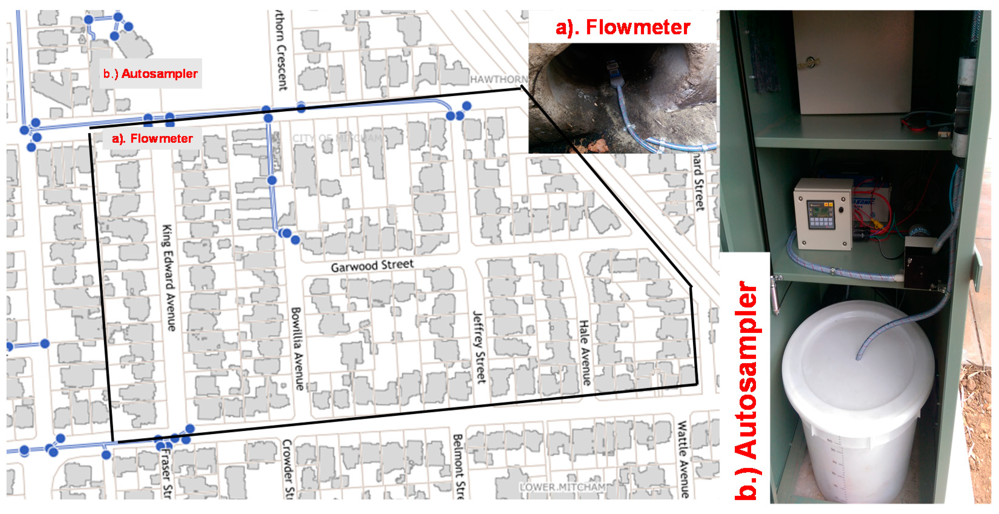
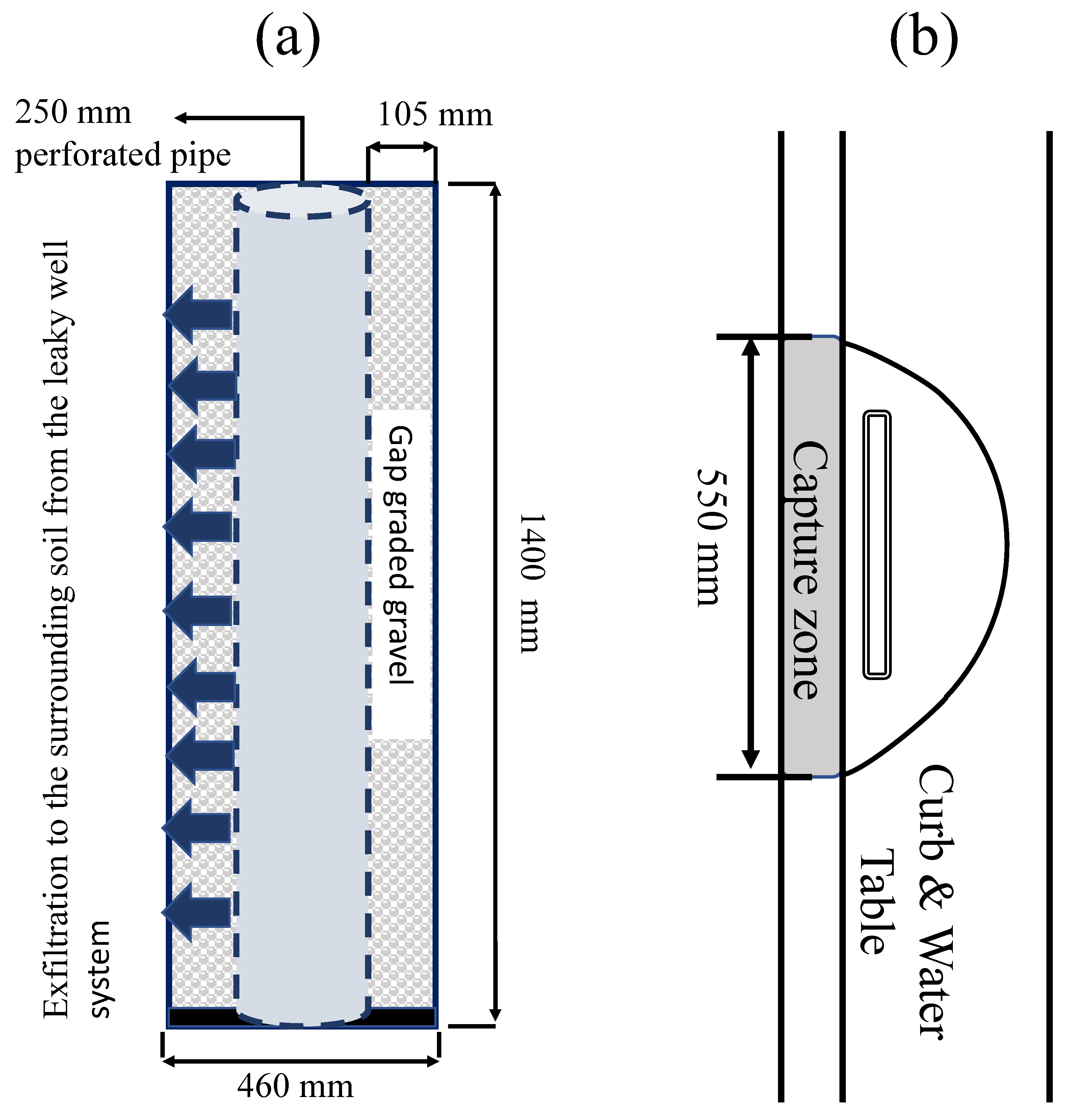
2.1. Catchment and Curbside Leaky Well Description
2.2. Monitoring Equipment
2.3. Curbside Leaky Well Installation
2.4. Description of Data Collection
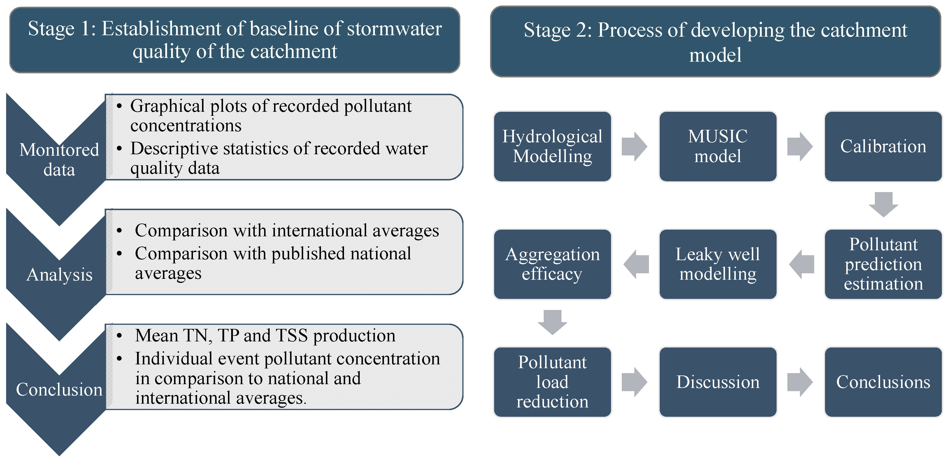
2.5. Catchment Model Development
2.5.1. Initial Parameter Section
2.5.2. Automated Calibration
2.6. Model Evaluation
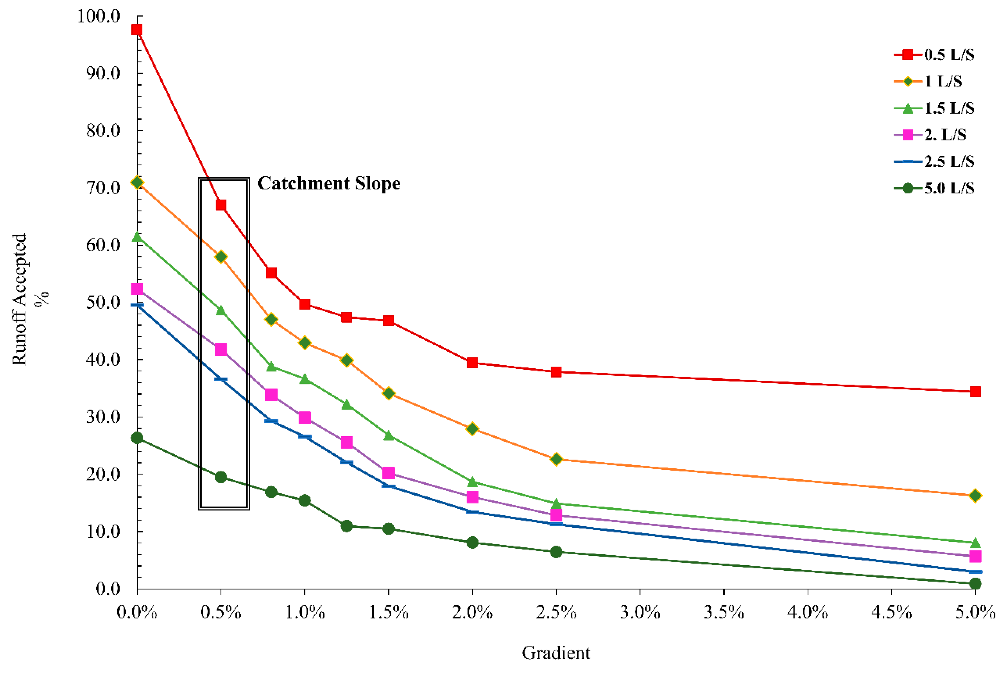
2.7. Infiltration Systems Modeling
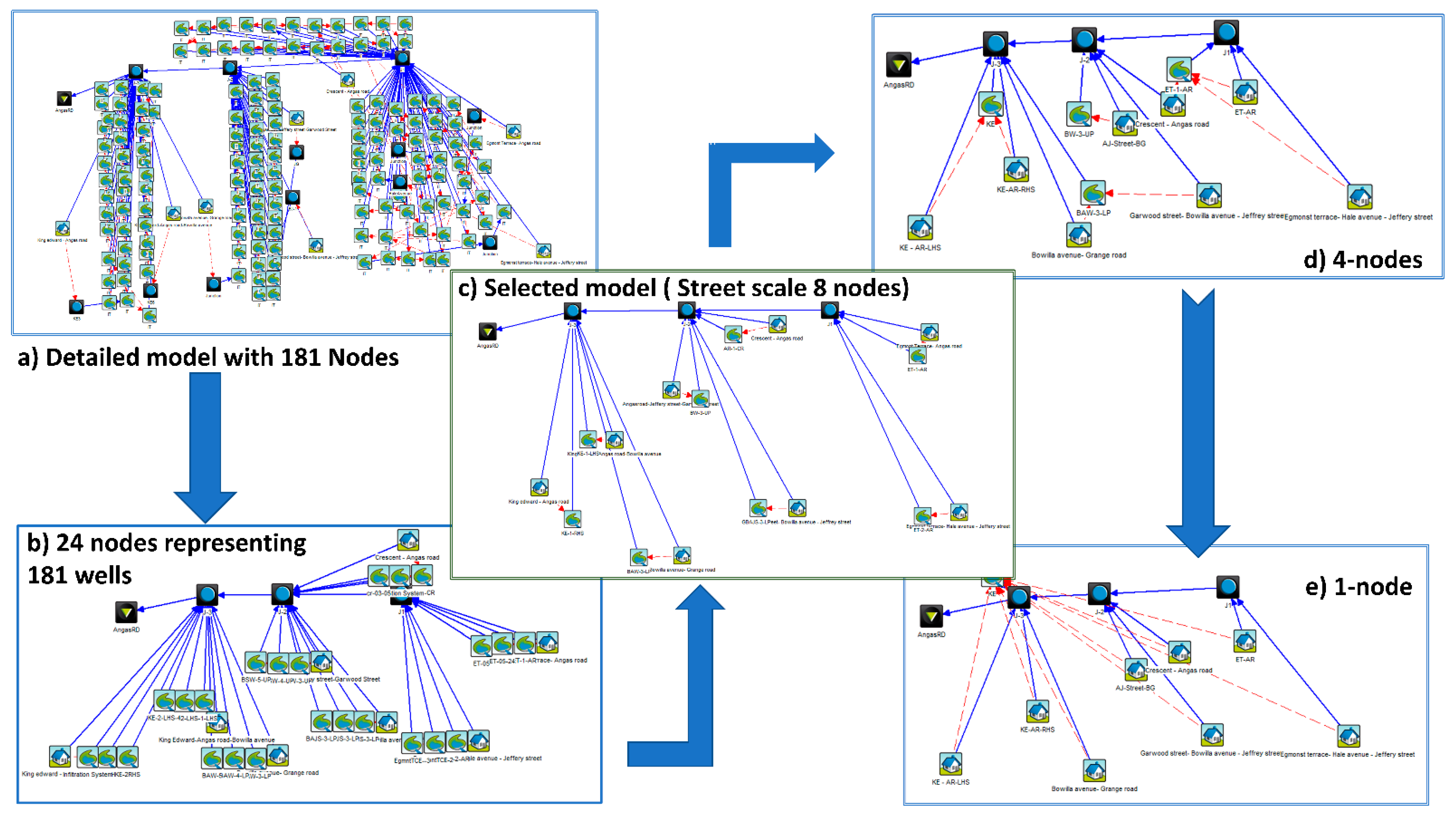
2.8. Examining the Impacts of Aggregating Infiltration Systems on Stormwater Quality
2.9. Water Quality Modeling
2.10. Data Analysis
3. Results
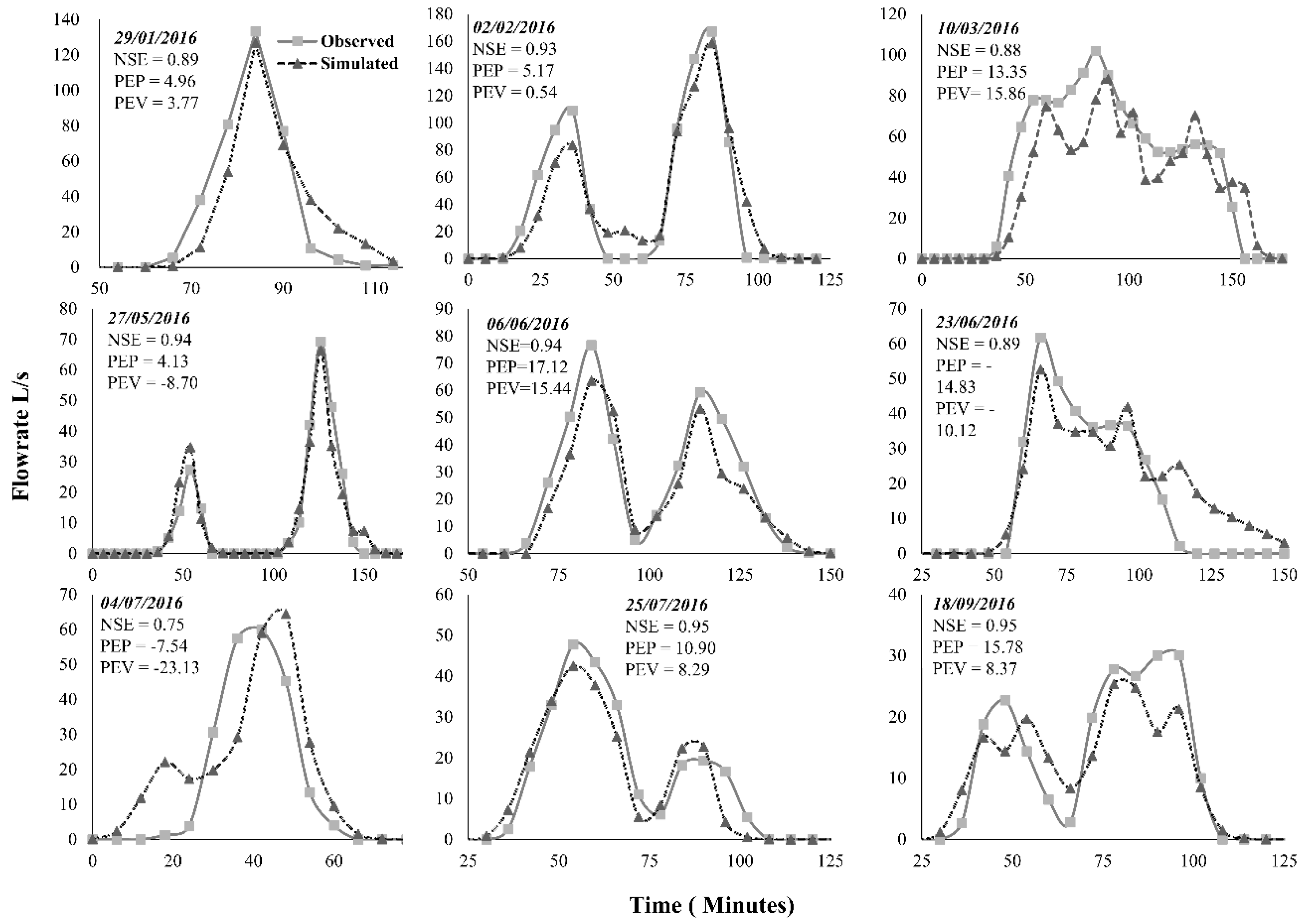
3.1. Model Calibration
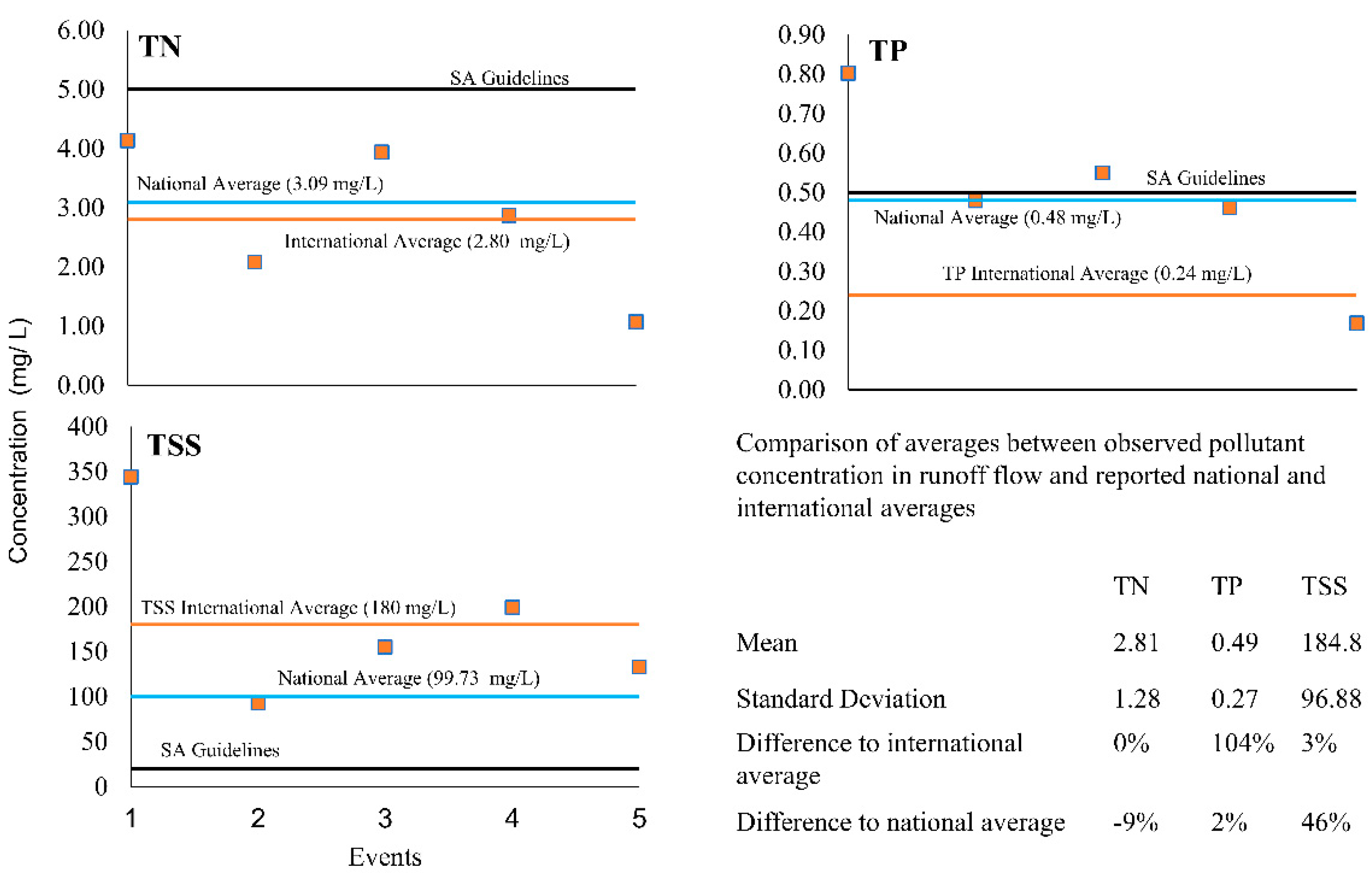
3.2. Water Quality Analysis
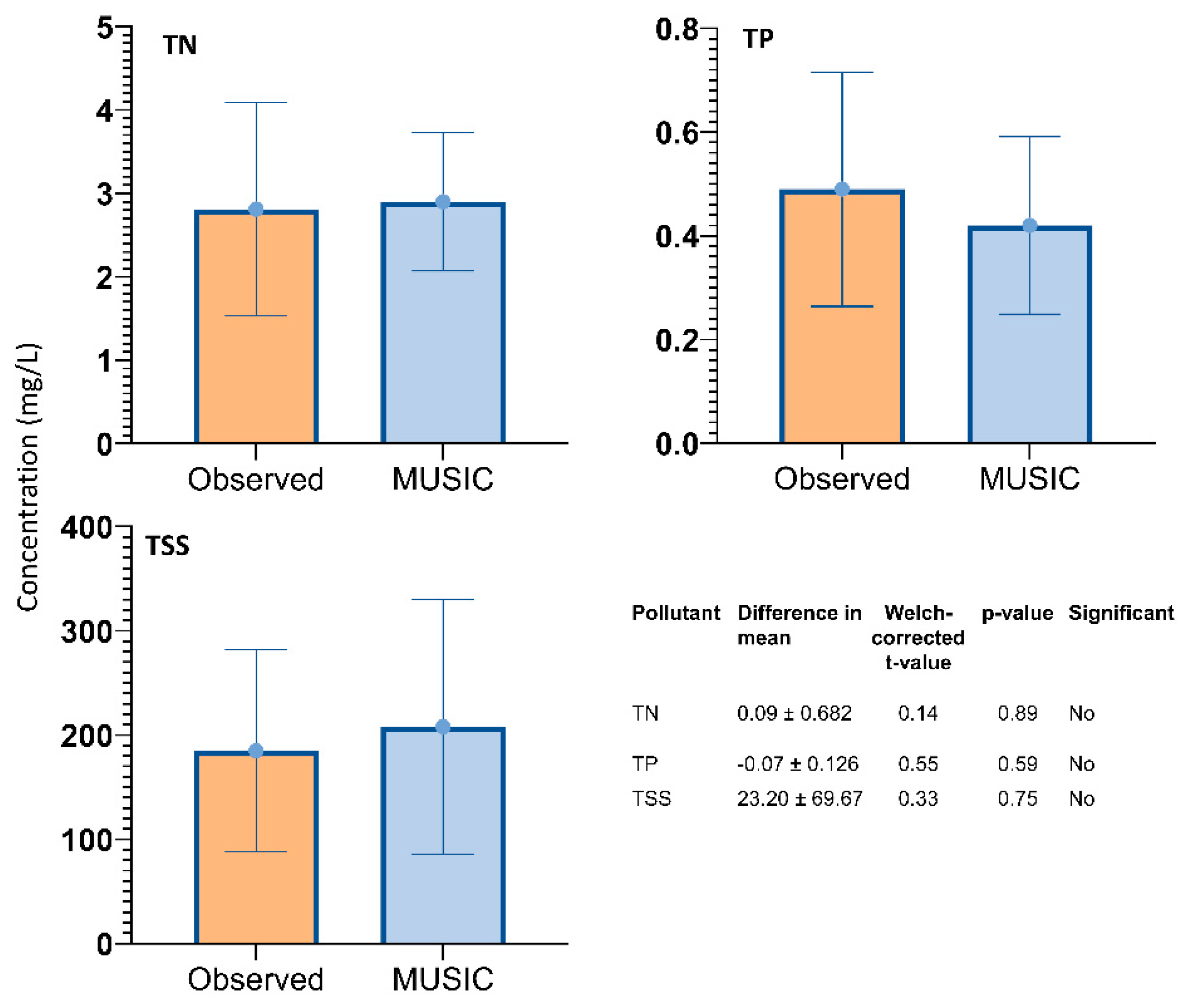
3.3. MUSIC Pollutant Predictions
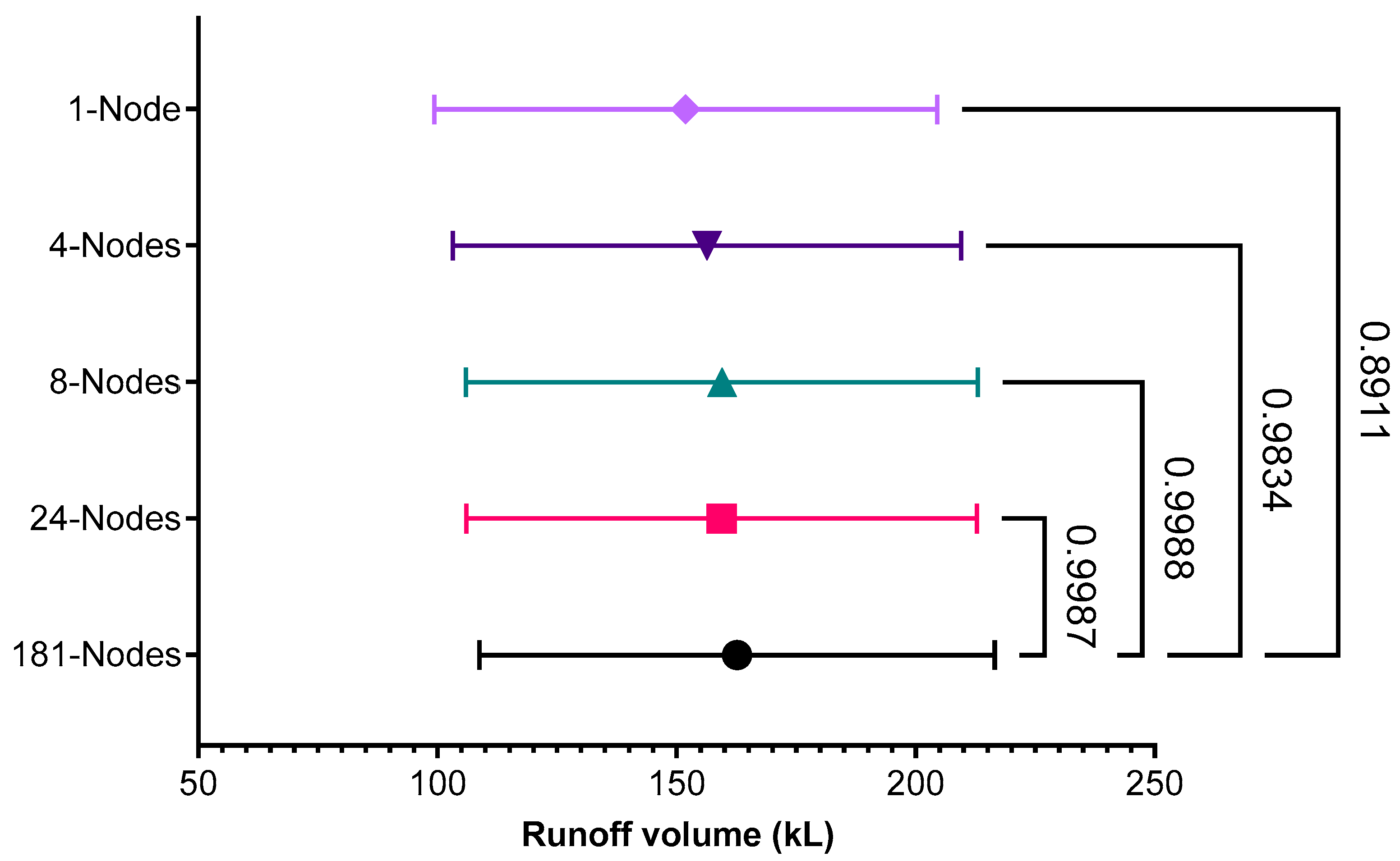
3.4. Leaky Well Aggregation
3.5. Performance of Leaky Wells to Reduce Pollutant Concentration in Catchment Outflows
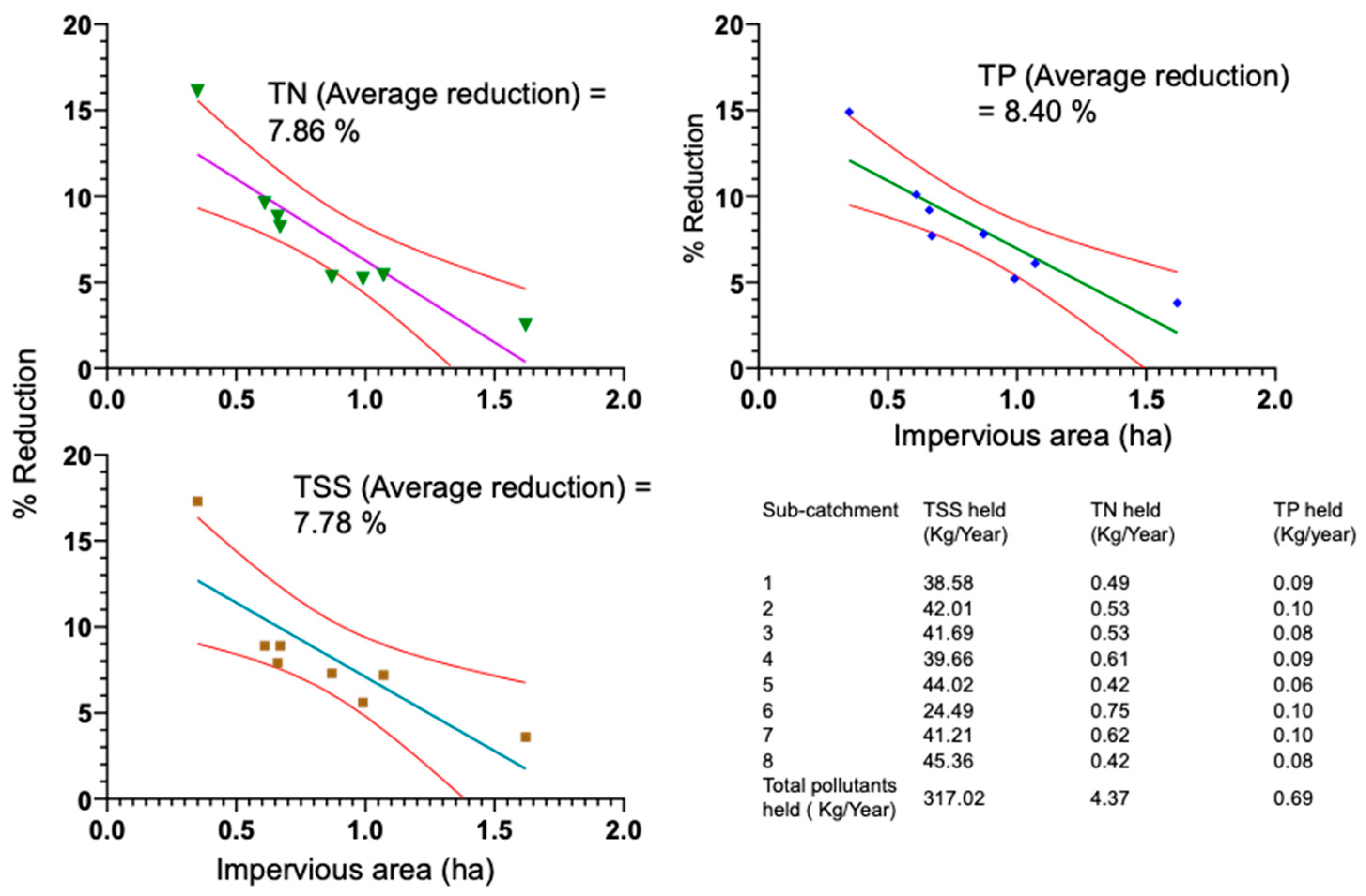
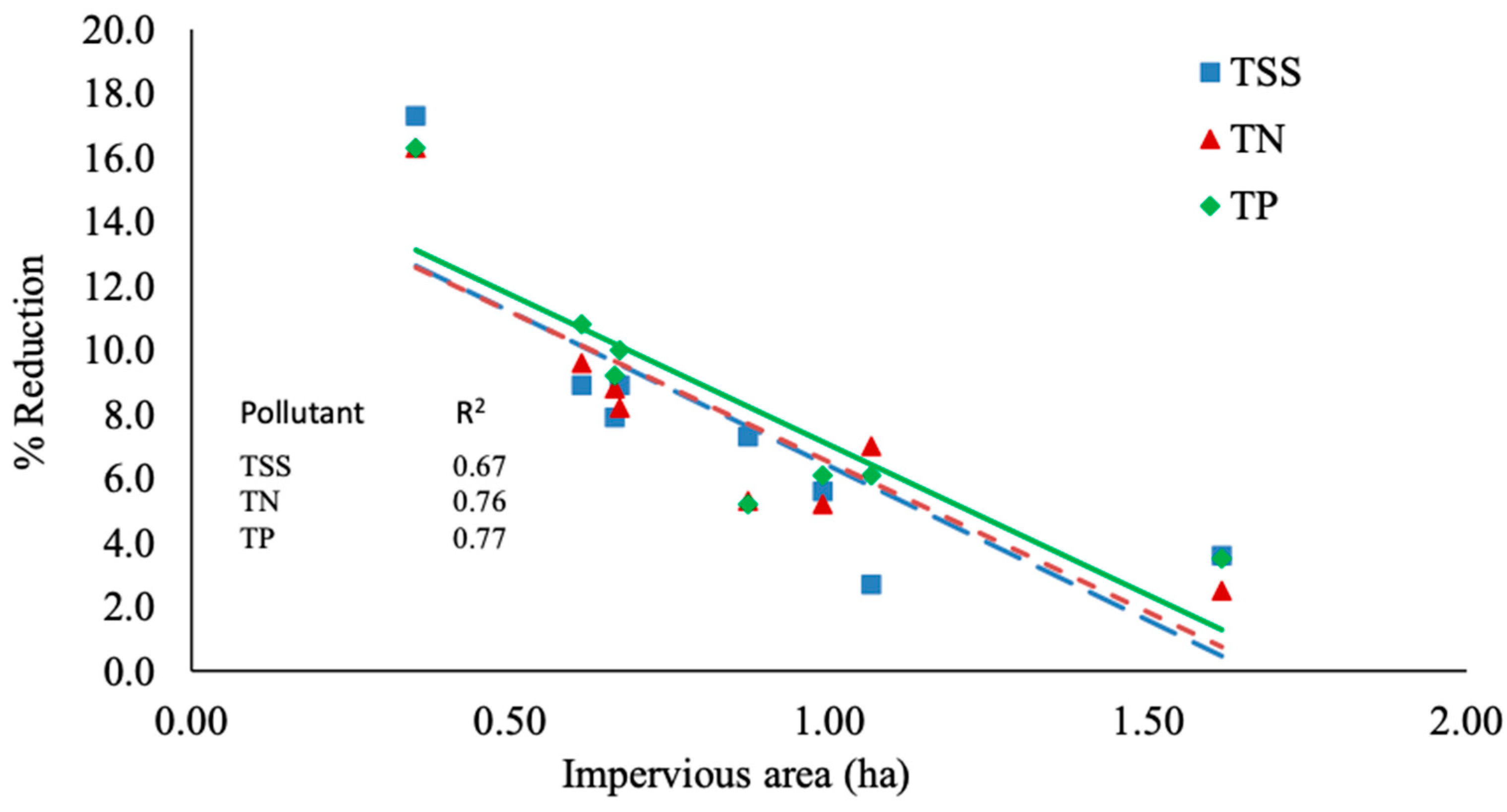
3.6. Impact of Connected Impervious Area
4. Discussion
4.1. Stormwater Quality of Catchment Outflows
4.2. Performance of MUSIC
4.3. Performance of Distributed Curbside Leaky Well Systems
5. Conclusions
Author Contributions
Funding
Data Availability Statement
Acknowledgments
Conflicts of Interest
References
- Bach, P.M.; Deletic, A.; Urich, C.; Sitzenfrei, R.; Kleidorfer, M.; Rauch, W.; McCarthy, D.T. Modelling interactions between lot-scale decentralised water infrastructure and urban form—A case study on infiltration systems. Water Resour. Manag. 2013, 27, 4845–4863. [Google Scholar] [CrossRef]
- Zhang, K.; Yong, F.; McCarthy, D.T.; Deletic, A. Predicting long term removal of heavy metals from porous pavements for stormwater treatment. Water Res. 2018, 142, 236–245. [Google Scholar] [CrossRef]
- Francey, M.; Fletcher, T.D.; Deletic, A.; Duncan, H. New insights into the quality of urban storm water in south eastern australia. J. Environ. Eng. 2010, 136, 381–390. [Google Scholar] [CrossRef]
- Lucke, T.; Drapper, D.; Hornbuckle, A. Urban stormwater characterisation and nitrogen composition from lot-scale catchments—New management implications. Sci. Total Environ. 2018, 619–620, 65–71. [Google Scholar] [CrossRef] [PubMed]
- Jani, J.; Yang, Y.-Y.; Lusk, M.G.; Toor, G.S. Composition of nitrogen in urban residential stormwater runoff: Concentrations, loads, and source characterization of nitrate and organic nitrogen. PLoS ONE 2020, 15, e0229715. [Google Scholar] [CrossRef] [Green Version]
- MacDonald, H.D.; Ardeshiri, A.; Rose, J.M.; Russell, B.D.; Connell, S.D. Valuing coastal water quality: Adelaide, south australia metropolitan area. Mar. Policy 2015, 52, 116–124. [Google Scholar] [CrossRef]
- Kuller, M.; Bach, P.M.; Ramirez-Lovering, D.; Deletic, A. Framing water sensitive urban design as part of the urban form: A critical review of tools for best planning practice. Environ. Model. Softw. 2017, 96, 265–282. [Google Scholar] [CrossRef]
- Todeschini, S.; Papiri, S.; Ciaponi, C. Placement strategies and cumulative effects of wet-weather control practices for intermunicipal sewerage systems. Water Resour. Manag. 2018, 32, 2885–2900. [Google Scholar] [CrossRef]
- Burns, M.J.; Fletcher, T.D.; Walsh, C.J.; Ladson, A.R.; Hatt, B.E. Hydrologic shortcomings of conventional urban stormwater management and opportunities for reform. Landsc. Urban Plan. 2012, 105, 230–240. [Google Scholar] [CrossRef]
- Fletcher, T.D.; Shuster, W.; Hunt, W.F.; Ashley, R.; Butler, D.; Arthur, S.; Trowsdale, S.; Barraud, S.; Semadeni-Davies, A.; Bertrand-Krajewski, J.-L.; et al. Suds, lid, bmps, wsud and more—The evolution and application of terminology surrounding urban drainage. Urban Water J. 2014, 12, 525–542. [Google Scholar] [CrossRef]
- Locatelli, L.; Mark, O.; Mikkelsen, P.S.; Arnbjerg-Nielsen, K.; Deletic, A.; Roldin, M.; Binning, P.J. Hydrologic impact of urbanization with extensive stormwater infiltration. J. Hydrol. 2017, 544, 524–537. [Google Scholar] [CrossRef] [Green Version]
- Sapdhare, H.; Myers, B.; Beecham, S.; Brien, C.; Pezzaniti, D.; Johnson, T. A field and laboratory investigation of kerb side inlet pits using four media types. J. Environ. Manag. 2019, 247, 281–290. [Google Scholar] [CrossRef]
- Roldin, M.; Fryd, O.; Jeppesen, J.; Mark, O.; Binning, P.J.; Mikkelsen, P.S.; Jensen, M.B. Modelling the impact of soakaway retrofits on combined sewage overflows in a 3 km2 urban catchment in copenhagen, denmark. J. Hydrol. 2012, 452, 64–75. [Google Scholar] [CrossRef]
- Fry, T.J.; Maxwell, R.M. Evaluation of distributed bmp s in an urban watershed—high resolution modeling for stormwater management. Hydrol. Processes 2017, 31, 2700–2712. [Google Scholar] [CrossRef]
- Zhang, K.; Bach, P.M.; Mathios, J.; Dotto, C.B.S.; Deletic, A. Quantifying the benefits of stormwater harvesting for pollution mitigation. Water Res. 2020, 171, 115395. [Google Scholar] [CrossRef]
- Sharma, A.; Pezzaniti, D.; Myers, B.; Cook, S.; Tjandraatmadja, G.; Chacko, P.; Chavoshi, S.; Kemp, D.; Leonard, R.; Koth, B.; et al. Water sensitive urban design: An investigation of current systems, implementation drivers, community perceptions and potential to supplement urban water services. Water 2016, 8, 272. [Google Scholar] [CrossRef] [Green Version]
- Bach, P.M.; Rauch, W.; Mikkelsen, P.S.; McCarthy, D.T.; Deletic, A. A critical review of integrated urban water modelling—Urban drainage and beyond. Environ. Model. Softw. 2014, 54, 88–107. [Google Scholar] [CrossRef]
- EWater. Music by Ewater: User Manual Version 5.0; Cooperative Research Centre: Canberra, Australia, 2014. [Google Scholar]
- Duncan, H. Urban stormwater quality: A statistical overview. In Australian Runoff Quality: A Guide to Water Sensitive Urban Design; Wong, T.H.F., Ed.; Engineers Australia: Barton, Australia, 2006. [Google Scholar]
- Water Sensitive South Australia and Adelaide and Mount Lofty Ranges Natural Resources Management Board. South Australia Music Guidelines. Adelaide, Australia. 2020. Available online: https://www.watersensitivesa.com/wp-content/uploads/SA-MUSIC-Guidelines-15Feb21-FINAL-DRAFT-for-website-22Mar21.pdf (accessed on 6 November 2021).
- Elliott, A.H.; Trowsdale, S.A.; Wadhwa, S. Effect of aggregation of on-site storm-water control devices in an urban catchment model. J. Hydrol. Eng. 2009, 14, 975–983. [Google Scholar] [CrossRef]
- Bureau of Meteorology. Design Rainfall Data System (2016); Meteorology, B.O., Ed.; Common Wealth of Australia: Australia, 2019; Volume 2019. [Google Scholar]
- Johnson, T.; Lawry, D.; Sapdhare, H. The council verge as the next wetland: Treenet and the cities of mitcham and salisbury investigate. In 29th International Horticultural Congress on Horticultural: Sustaining Lives, Livelihoods and Landscapes; International Society for Horticultural Science: Birsbane, Australia, 2016; Volume 1, pp. 63–69. [Google Scholar]
- Doherty, J. Pest: A unique computer program for model-independent parameter optimisation. In Water Down Under 94: Groundwater/Surface Hydrology Common Interest Papers; Preprints of Papers; Institution of Engineers: Barton, ACT, Australia, 1994; pp. 551–554. [Google Scholar]
- Dotto, C.B.; Deletic, A.; Fletcher, T.D. Analysis of parameter uncertainty of a flow and quality stormwater model. Water Sci Technol. 2009, 60, 717–725. [Google Scholar] [CrossRef]
- ASCE Task Committee. Asce task committee on definition of criteria for evaluation of watershed models of the watershed management committee, irrigation, drainage division, criteria for evaluation of watershed models. J. Irrig. Drain. Eng. 1993, 119, 429–442. [Google Scholar]
- Moriasi, D.N.; Gitau, M.W.; Pai, N.; Daggupati, P. Hydrologic and water quality models: Performance measures and evaluation criteria. Trans. ASABE 2015, 58, 1763–1785. [Google Scholar]
- Natrual Resource Management Ministerial Council; Envrionmental Protection and Heritage Council; National Health and Medical Research Council. In Australian Guidelines for Water Recycling; National Water Quality Management Strategy; Canberra, Australia; 2009. Available online: https://www.waterquality.gov.au/sites/default/files/documents/water-recycling-guidelines-stormwater-23.pdf (accessed on 6 November 2021).
- Environment Protection Authority SA. Environment Protection (Water Quality) Policy 2003 and Explanatory Report; Environment Protection Authority SA, Ed.; Goverment of South Australia: Adelaide, Australia, 2003. [Google Scholar]
- Gustafson, K.R.; Garcia-Chevesich, P.A.; Slinski, K.M.; Sharp, J.O.; McCray, J.E. Quantifying the effects of residential infill redevelopment on urban stormwater quality in denver, colorado. Water 2021, 13, 988. [Google Scholar] [CrossRef]
- Alam, M.Z.; Anwar, A.H.M.F.; Sarker, D.C.; Heitz, A.; Rothleitner, C. Characterising stormwater gross pollutants captured in catch basin inserts. Sci. Total Environ. 2017, 586, 76–86. [Google Scholar] [CrossRef] [PubMed]
- Müller, A.; Österlund, H.; Marsalek, J.; Viklander, M. The pollution conveyed by urban runoff: A review of sources. Sci. Total Environ. 2020, 709, 136125. [Google Scholar] [CrossRef] [PubMed]
- Yarmoshenko, I.; Malinovsky, G.; Baglaeva, E.; Seleznev, A. A landscape study of sediment formation and transport in the urban environment. Atmosphere 2020, 11, 1320. [Google Scholar] [CrossRef]
- Myers, B.; Pezzaniti, D.; Kemp, D.; Chavoshi, S.; Montazeri, M.; Sharma, A.; Chacko, P.; Hewa, G.A.; Tjandraatmadja, G.; Cook, S. Water Sensitive Urban Design Impediments and Potential: Contributions to the Urban Water Blueprint (Phase 1): Task 3: The Potential Role of Wsud in Urban Service Provision; Goyder Institute for Water Research: Adelaide, Australia, 2014. [Google Scholar]
- Myers, B.; Cook, S.; Maheepala, S.; Pezzaniti, D.; Beecham, S.; Tjandraatmadja, G.; Sharma, A.; Hewa, G.; Neumann, L. Interim Water Sensitive Urban Design Targets for Greater Adelaide; Goyder Institute for Water Research: Adelaide, Australia, 2011. [Google Scholar]


| Parameter | Value | Method of Estimation | SA Guidelines for MUSIC Modelling [20] |
|---|---|---|---|
| Sub catchments | 8—Urban nodes | Lumped Approach | Section 4.1 |
| Area (ha) | 0.8 to 4.04 | GIS map available | |
| Imperviousness | 28~43% | GIS map. The imperviousness was based on the subtraction of indirectly connected impervious area total impervious, for conservative estimate. | Section 4.2.2, recommends estimating for impervious fractions based on available plans |
| Rainfall threshold (mm/day) | 4.0~5.0 | Calibration using PEST, Values varies from 1 mm/day to maximum of 5 mm/day as recommended in MUSIC manual | No specific information is available to select this parameter |
| Soil storage capacity (mm) | 102 | Used in calibration by providing range of 88 mm to 108 mm, based on recommended values for light clays in SA Guidelines for Music modelling | Section 4.3 |
| Field capacity (mm) | 69 | Used in calibration by providing range of 63 mm to 83 mm, based on recommended values for light clays | Section 4.3 |
| Infiltration capacity coefficient—a (mm/day) | 145 | Used in calibration by providing range of 125 mm to 145 mm, based on recommended values for light clays | Section 4.3 |
| Infiltration capacity coefficient—b (mm/day) | 0.5 | Used in calibration by providing range of 0.5 mm to 4 mm, based on minimum and maximum values for different soil groups | Section 4.3 |
| Parameters | Detailed Model | Aggregation Methodology |
|---|---|---|
| No of infiltration wells for each sub-catchment | 181 nodes are modeled | Five levels of aggregation, based on combining wells in series in one street, street scale aggregation, combining all wells in one node |
| Inlet Properties—Low Flow By-pass (L/s) | Every low flow is assumed to be captured by the inlet | Aggregation should not impact the low flow bypass |
| Inlet Properties—High Flow By-pass (L/s) | Based on laboratory trials | Consider same for aggregated systems as well. Although this would change, however, as noticed the model was not sensitive to this parameter. |
| Storage and Infiltration Properties—Pond Surface Area (square meters) | Based on Excavated holes for the well | Sum of contributing nodes |
| Storage and Infiltration Properties—Extended Detention Depth (meters) | Based on length of inlet pipe | Inlet pipe remained same to reflect the similar capture efficiency of leaky wells. |
| Storage and Infiltration Properties—Filter Area (square meters) | Total area of the well based on excavated holes of 460 mm diameter | Sum of contributing nodes |
| Storage and Infiltration Properties—Unlined Filter Media Perimeter (meters) | Circumference of excavated hole | Sum of circumference of contributing nodes |
| Storage and Infiltration Properties—Depth of Infiltration Media (meters) | Maximum depth | Kept same as of individual systems to preserve the hydraulic head |
| Pollutant | Range (mg/L) [19] | International Water Quality Mean (mg/L) [19] | National Water Quality Mean (mg/L) [28] | SA Guidelines for Receiving Waterbodies [29] |
|---|---|---|---|---|
| TSS | 50–500 | 180 | 99.73 | 20 |
| TN | 1.8–5.5 | 2.8 | 3.09 | 5 |
| TP | 0.08–0.8 | 0.24 | 0.480 | 0.5 |
| Event | NSE | PEP | PEV | Evaluation Based on NSE |
|---|---|---|---|---|
| 29 January 2016 | 0.89 | 4.96 | 3.77 | Very Good |
| 2 February 2016 | 0.93 | 5.17 | 0.54 | Very Good |
| 10 March 2016 | 0.88 | 13.35 | 15.86 | Very Good |
| 27 May 2016 | 0.94 | 4.13 | 8.70 | Very Good |
| 6 June 2016 | 0.90 | 1.37 | −10.12 | Very Good |
| 23 June 2016 | 0.87 | −14.83 | 10.25 | Very Good |
| 4 July 2016 | 0.75 | −7.54 | −23.13 | Good |
| 25 July 2016 | 0.95 | 10.90 | 8.29 | Very Good |
| 18 September 2016 | 0.95 | 15.78 | 8.37 | Very Good |
| Parameters | Wells Aggregated | |||
|---|---|---|---|---|
| Contributing wells to each node | 7.54 | 22.63 | 45.25 | 181 |
| Inlet Properties—Low Flow By-pass (m3/s) | 0 | 0 | 0 | 0 |
| Inlet Properties—High Flow By-pass (L/sec) | 5 | 5 | 5 | 5 |
| Storage and Infiltration Properties—Pond Surface Area (m2) | 1.2 | 3.62 | 7.24 | 28.96 |
| Storage and Infiltration Properties—Extended Detention Depth (m) | 0.15 | 0.15 | 0.15 | 0.15 |
| Storage and Infiltration Properties—Filter Area (m2) | 1.2 | 3.62 | 7.24 | 28.96 |
| Storage and Infiltration Properties—Unlined Filter Media Perimeter (m) | 10.86 | 32.54 | 65.16 | 260.64 |
| Nodes | Runoff Volume—Total Period (kL) | Difference in Comparison to Preinstallation Scenario | Mean Annual Runoff Volume (kL) | Standard Deviation |
|---|---|---|---|---|
| 181 | 6669.63 | 4% | 162.67 | 53.89 |
| 24 | 6535.56 | 6% | 159.40 | 53.38 |
| 8 | 6531.56 | 6% | 159.31 | 53.55 |
| 4 | 6410.40 | 7% | 156.35 | 53.17 |
| 1 | 6228.13 | 10% | 151.91 | 52.59 |
Publisher’s Note: MDPI stays neutral with regard to jurisdictional claims in published maps and institutional affiliations. |
© 2021 by the authors. Licensee MDPI, Basel, Switzerland. This article is an open access article distributed under the terms and conditions of the Creative Commons Attribution (CC BY) license (https://creativecommons.org/licenses/by/4.0/).
Share and Cite
Shahzad, H.; Myers, B.; Hewa, G.; Johnson, T.; Boland, J.; Mujtaba, H. Characterizing the Stormwater Runoff Quality and Evaluating the Performance of Curbside Infiltration Systems to Improve Stormwater Quality of an Urban Catchment. Water 2022, 14, 14. https://doi.org/10.3390/w14010014
Shahzad H, Myers B, Hewa G, Johnson T, Boland J, Mujtaba H. Characterizing the Stormwater Runoff Quality and Evaluating the Performance of Curbside Infiltration Systems to Improve Stormwater Quality of an Urban Catchment. Water. 2022; 14(1):14. https://doi.org/10.3390/w14010014
Chicago/Turabian StyleShahzad, Hussain, Baden Myers, Guna Hewa, Tim Johnson, John Boland, and Hassan Mujtaba. 2022. "Characterizing the Stormwater Runoff Quality and Evaluating the Performance of Curbside Infiltration Systems to Improve Stormwater Quality of an Urban Catchment" Water 14, no. 1: 14. https://doi.org/10.3390/w14010014
APA StyleShahzad, H., Myers, B., Hewa, G., Johnson, T., Boland, J., & Mujtaba, H. (2022). Characterizing the Stormwater Runoff Quality and Evaluating the Performance of Curbside Infiltration Systems to Improve Stormwater Quality of an Urban Catchment. Water, 14(1), 14. https://doi.org/10.3390/w14010014