Isotopic Assessment of Groundwater Salinity: A Case Study of the Southwest (SW) Region of Punjab, India

Abstract

In recent decades, due to rapid increases in water demand and greater usage of water for irrigation from surface canals, waterlogging problems have been created in the southwest zone of Punjab, coupled with a stagnation in saline zone formation due to salinity ingression. To understand these salinity issues, the present study has been conducted in three districts (Muktsar, Fazilka, and Faridkot) of Punjab to understand the root cause. To this end, groundwater samples were collected from 142 piezometers developed at 40 sites. Electrical conductivity (EC) observations were taken in the field, and collected samples were analyzed for isotopes in the laboratory. Results found that salinity in groundwater arises from the combination of evaporation enrichment and salt dissolution. The dissolved salts may be acquired due to salts from aquifer materials or salts from surface soils dissolving and leaching down with the recharging water. Besides, the zone of interaction is mapped using stable isotopic composition. The study suggests that zone of interaction between aquifers can be effectively used in groundwater augmentation, management, and contamination control at regional and/or global scales to curb water demand in the future.

1. Introduction

Generally, groundwater is used for irrigation in arid and semi-arid regions of the India and fulfills the demands of the huge population, but in the southwest (SW) region of Punjab, surface water is used for irrigation thanks to well-developed canal networks. Bonsor et al. [1] stated that the Punjab state of India, having great hydrogeological characteristics, underlies Haryana, Rajasthan, Delhi, and Punjab, where groundwater depletes at a rate of 109 km³/year [2]. Further, it is a widely recognized state for groundwater utilization in India and is listed second in over-stressed aquifers globally [3]. In other parts of Punjab, such as the Indo-Gangetic basin, people rely heavily on groundwater, resulting in a rapid decline in the water demand, consequently impacting the quantity and quality of the water [1,4]. Groundwater salinity is also one of the quality issues [5] that has emerged in this region as a result of various factors [6,7]. Various approaches along with environmental isotopes have been found useful in finding the groundwater salinity’s causes and mechanisms [8,9,10,11]. Multi-aquifer systems developed due to diverse geological formations, as well as the levels of salinity in these aquifers, may vary due to geogenic as well as anthropogenic reasons [12]. In general, the salinity of the groundwater could be increasing due to adequate availability of nitrate, fluoride, iron, total hardness, arsenic, and some toxic metal ions (e.g., Cd, Ni, Pb) in several states of India, causing potential risks to human health [13,14,15,16]. In addition, if there is sufficient surface water availability, then inadequate use of groundwater leads to a rise in the groundwater level, resulting in waterlogging conditions that increase salinity [6,17]. In the SW region of Punjab, farmers copiously use canal water for irrigation, and in some parts, fluctuating groundwater levels have put water managers into a predicament in terms of separating the saline and freshwater zones.

In the modern era, stable isotopes (δ¹⁸O and δD) of water are widely used in hydrological studies for the identification of key sources of pollution and in other hydrological processes [18,19,20,21,22]. Besides, researchers of different works of life reported the application of environmental isotopes to identify the source of groundwater recharge and estimations of quality, quantity, dating, and their interconnections; seepage from tunnels, reservoirs, canals, etc.; contributions of snow-ice melt in glacier discharges; and nutrients, dynamics, and sedimentation in freshwater bodies (e.g., lakes, reservoirs) [23,24,25,26]. The relationship between δ¹⁸O and δD in freshwaters, i.e., δD = 8 × δ¹⁸O + 10 [27], and their function is called “d-excess” and is represented by d-excess = δD − 8 × δ¹⁸O. The value of d-excess varies due to evaporation at various stages [28]. The use of stable isotopes can be extremely useful in identifying various hydrological processes [6,29]; mechanisms [11]; sources [21,30]; characteristics of surface–groundwater interactions [22]; and depth-wise salinity variations [19] in India. In view of the above, the present study is carried out to (i) assess the present-day waterlogging and groundwater saline in aquifers at different depths in the southwest (SW) parts of Punjab and (ii) identify depth-wise saline water and freshwater zones in the aquifers using isotopes.

2. Materials and Methods

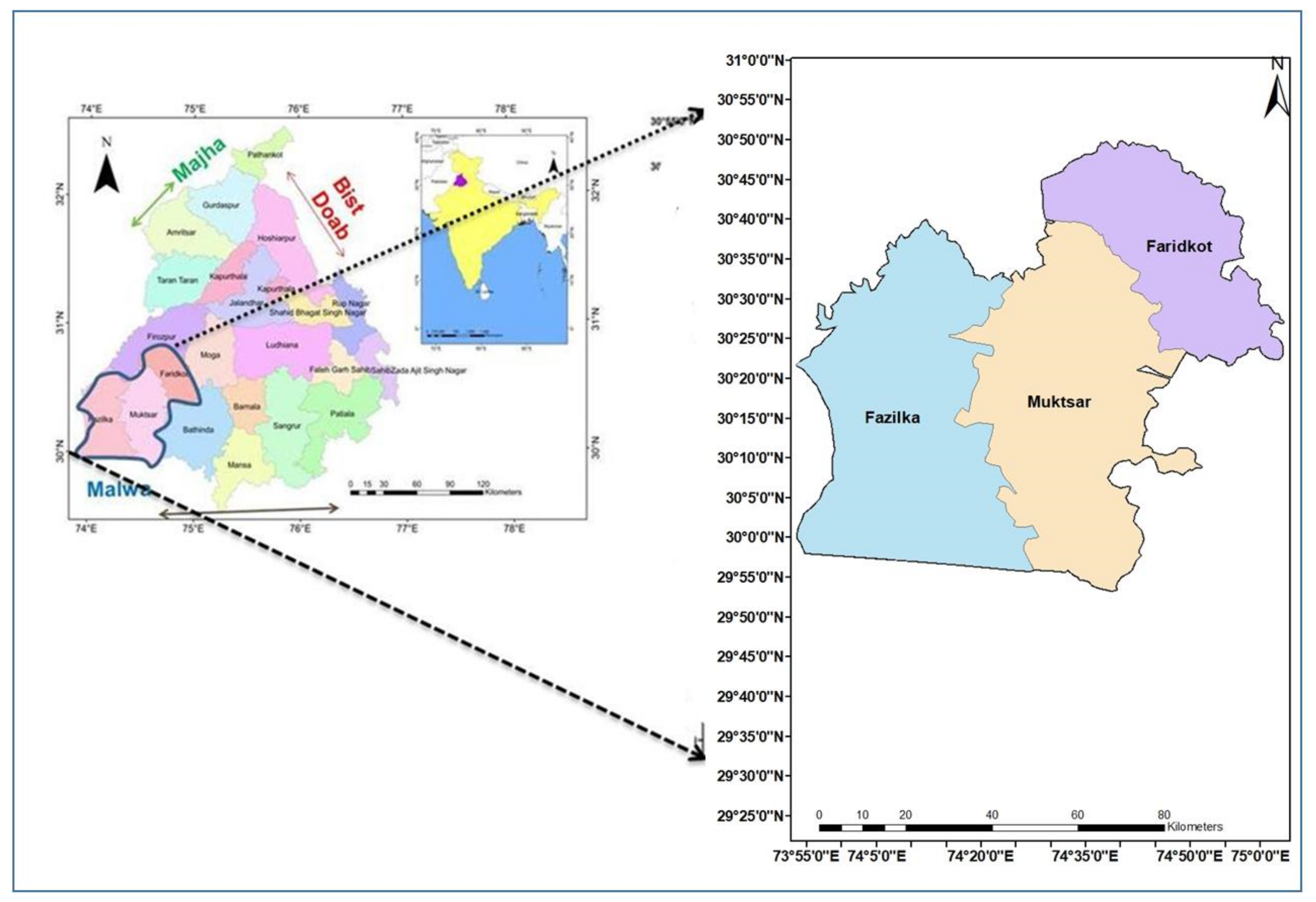
2.1. Study Area

The study was carried out in three districts, namely Fazilka, Muktsar, and Faridkot (Figure 1) of the SW region (Malwa) of Punjab, India, constituting a total land area of about 6932 km². The geographical location of the study area lies between latitudes 29°54′20″ N and 30°49′52″ N and longitudes 73°52′4″ E and 75°03′22″ E. There are a total of 10 administrative blocks, with 4 distributed in the Fazilka district, 4 in the Muktsar district, and 2 in the Faridkot district. The study area shares an international boundary with Pakistan to the west and a state boundary with Rajasthan to the south, and within the state of Punjab, the Bhatinda district is to the east, and the districts of Firozpur and Moga are to the north. Physio-graphically, it is in the Sutlej sub-basin and is covered extensively by the Sutlej Canal network, including Indira Gandhi Canal and Ganga Canal (Bikaner Canal), two major canals of the state of Rajasthan.

2.1.1. Demography

As per the census 2011 [31], the study area, comprised of 3 districts, had a population of 2.7 million, with a share of 9.73% (10%) of Punjab state’s population living within, and during 2001–2011, districts Faridkot, Fazilka, and Muktsar had population growth rates of 12.18%, 13.12%, and 16.1%; average population densities of 424, 380, and 348 persons per square kilometer (km²), which are greater than the national average of 327 persons/km²; sex ratios (female/male) of 889/1000, 923/1000, and 895/1000; and literacy rates of 70.6%, 70.7%, and 66.8%, respectively.

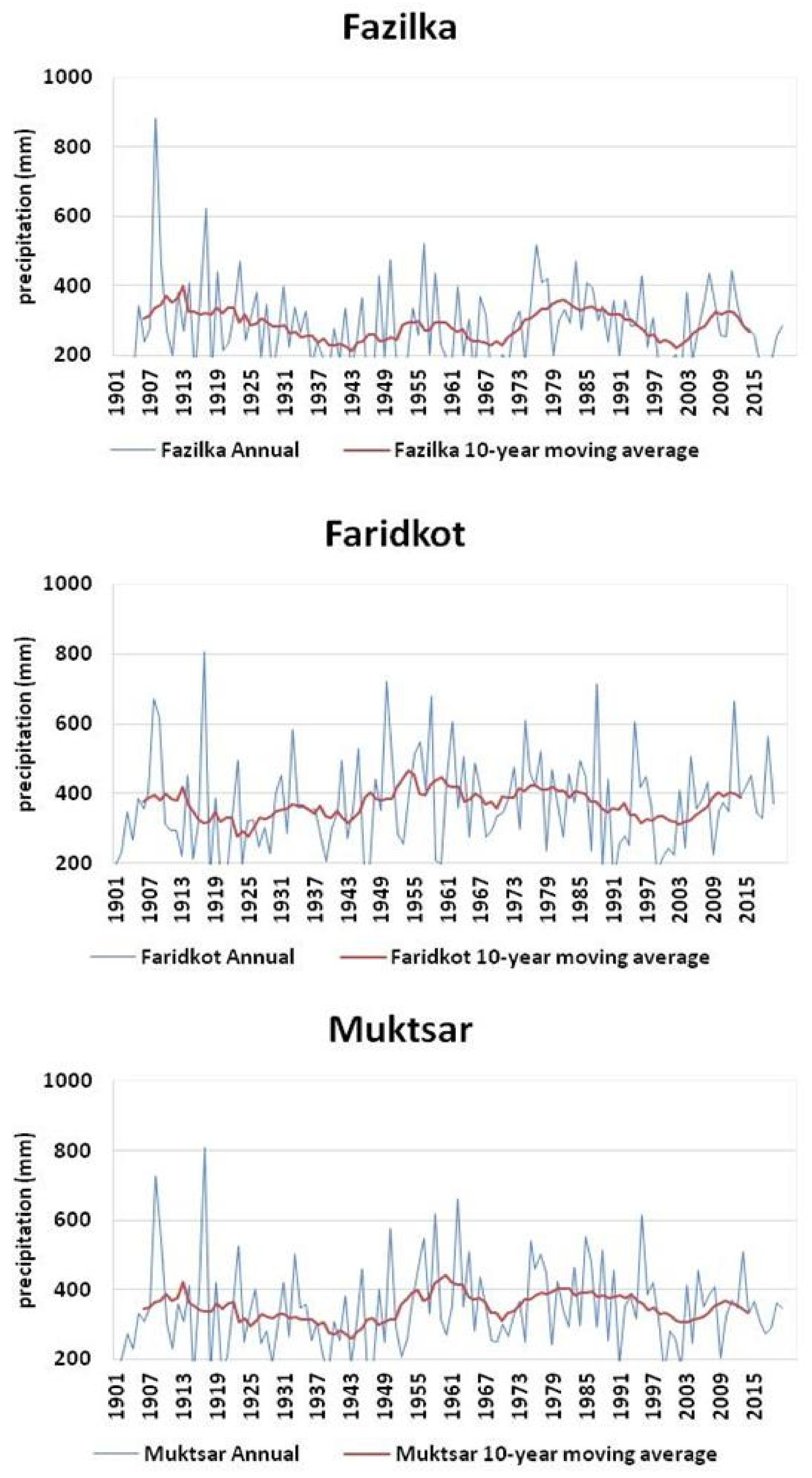
2.1.2. Hydrogeology and Climate

In this study, very high spatial resolution daily gridded rainfall data (0.25 × 0.25 degree) have been taken from the Indian Metrological Department (IMD, Pune) for the period of 1901 to 2019 and plotted in Figure 2. The normal annual rainfall is 449 mm, and 80% of it occurs during the SW monsoon season. The study area is a part of Sutlej Basin and developed by Indo-Gangetic alluvium, with alluvial plains occupying maximum area, followed by sand sheets and sand dunes as patches. Evidence shows that a paleochannel exists in the central part of the Faridkot district, and there are sequences of Quaternary deposits of Mid-Pleistocene to Recent age, comprising fluvial and arid phases in an alternate manner. The older alluvium originates from the Himalayas, and recent Aeolian deposits have been laid down by the action of wind from the Thar Desert of Rajasthan. The study area is underlain by a multi-aquifer system formed by intermittent layers of clay and a number of granular layers (Figure 3), which extends to a depth of up to 300 m. The aquifers are composed of fine- to coarse-grained sand, further separated by a 25–40 m thick clay zone [32]. The first aquifer (composed of fine- to coarse-grained sand) is a water table aquifer and extends all over the area.

2.1.3. Agriculture and Irrigation

Agriculture is the major occupation in the study area, with two main cropping seasons of July to December (Kharif) (maize, bajra, paddy, cotton, mash, moong, arhar, moth, sugarcane, etc.) and December to April (Rabi) (barley, gram, wheat, taramera, sarson, toria, etc.) in a year. Major sources of irrigation are surface water and groundwater, but due to the issues of groundwater salinity, canal water is largely used to fulfill irrigation needs.

2.2. Methodologies Adopted

For separating out the zone of freshwater and saline water horizontally as well as vertically, the Department of Agriculture & Farmers’ Welfare (DAFW), Punjab has constructed a network of depth-specific piezometers at 40 sites in consultation with the National Institute of Hydrology (NIH), Roorkee in the study area (Figure 4).

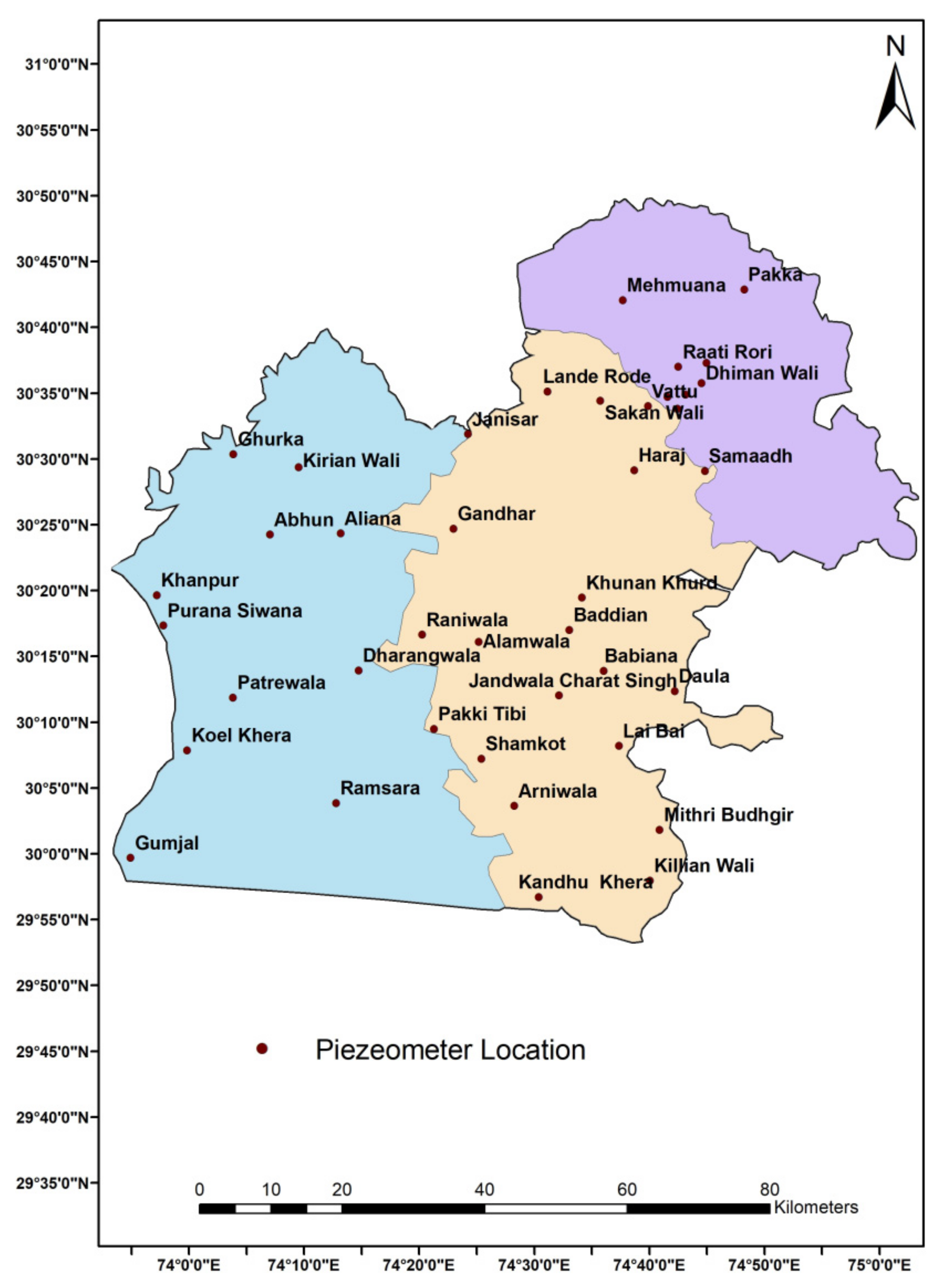
2.2.1. Piezometer Construction

Depth-specific piezometer construction was carried out at sites shown in Figure 4 using the standard methodology. The site selection for the installation of clusters of piezometers was done by DAFW, Punjab. Based on the evaluation of available geological information, the locations of boreholes and the collection zones were carefully selected in constructing the piezometers. In this study, 250 mm (10 in) drilling was done below the proposed location of the piezometer, the top and bottom parts were filled with clean, fine sand, and bentonite was used for sealing.

2.2.2. Sampling and Analysis

Groundwater samples were collected in three campaigns from the newly drilled depth-specific piezometers during November–December 2019 (6 sites); February 2021 (16 sites); and August 2021 (18 sites). To avoid errors, samples were carefully collected in triplicate in fresh, clean, and dry LDPE (low-density polyethylene) Tarson bottles for the laboratory analysis of stable isotopes (δ¹⁸O and δD). Collected samples were transported in ice boxes and preserved at 4 °C before analysis [34,35]. Prior to sampling, on-site analyses of pH and electrical conductivity (EC) were done using portable instruments (pH meter and Eutech portable EC, respectively).

The stable isotopic ratios (δ¹⁸O and δD) were measured by dual-inlet isotope ratio mass spectrometer (DI-IRMS) (Isoprime GV instruments, Cheadle, UK) with a precision of ±0.1‰ for δ¹⁸O and ±1.0‰ for δD. In dual-inlet IRMS, the inlet is alternately switched for analysis between standard and reference gas by adjusting their volumes with the help of changeover valve to obtain matching pressure, which helps in improving accuracy. For deuterium analysis and oxygen analysis, hydrogen gas in the presence of a platinum catalyst and CO₂ are equilibrated at 40 °C for 7 h and 2.5 h, respectively, and then filled into the sample bellow after being dehydrated by passing through a cold finger. Reference gas is pre-filled into the reference bellow, and equal volumes of sample gas and reference gas are alternately purged into the mass spectrometer for isotopic analysis.

All spatially varying databases were analyzed by the ARC/GIS tool (version 10.1). In the present study, groundwater samples were collected from 142 newly developed piezometers by the Department of Agriculture & Farmers’ Welfare, Punjab at 40 sites, and the respective isotopic values (δD and δ¹⁸O) were measured.

Measurement and Analysis of Groundwater Salinity

Groundwater salinity is generally of 3 types [6]: (i) natural/primary salinity; (ii) dryland/secondary salinity; and (iii) tertiary/irrigated salinity. Based on the origin of salinity, it may be classified as [36] (i) marine origin; (ii) terrestrial origin—natural, due to processes of evaporation, dissolution, etc.; (iii) terrestrial origin—anthropogenic reasons; or (iv) mixed origin. Electrical conductivity (EC—µS/cm) of groundwater samples was measured and was also used to compute total dissolved solids (TDS in mg/L) by applying calculations as given below:

$$\mathrm{TDS}=\mathrm{EC}\times 0.64 \mathrm{EC} \mathrm{ranges} \mathrm{from} 100 \mathrm{to} 5000 \mu \mathrm{S}/\mathrm{cm}$$

(1)

$$\mathrm{TDS}=\mathrm{EC}\times 0.64 \mathrm{when} \mathrm{EC} > 5000 \mu \mathrm{S}/\mathrm{cm}$$

(2)

Water is defined to be freshwater at salt concentration < 1000 mg/L, potable for drinking at <500 mg/L for palatability. The permissible limit of salinity for drinking water is 2000 mg/L, and beyond that, it is considered saline [37].

Measurements of Stable Isotopes

Measurements of stable isotopes are done in terms of abundance ratios, i.e., atomic mass of heavy atom to the atomic mass of light atom. Only the relative difference in the ratio of the heavy isotopes to the more abundant light isotope of the sample, with respect to a reference, is determined. The difference is designated by a Greek letter δ and is defined as follows:

δ = (R_sample − R_reference)/R_reference

(3)

where Rs denote the ratios of ¹⁸O/¹⁶O and D/H isotopes in the case of water.

The difference between samples and references is usually quite small, and δ values are therefore expressed in per mille differences (‰), i.e., per thousand.

δ (‰) = δ × 1000

(4)

δ (‰) = [(R_s − R_r)/R_r] × 10 ³ = [(R_s/R_r) − 1] × 10³

(5)

If the δ value is positive, it refers to the enrichment of the sample in the heavy isotope species, with respect to the reference, and the negative value corresponds to the sample depleted in the heavy isotope species.

The relation between δD and δ¹⁸O can be written in a standard form (equation for straight line):

δD‰ = A δ¹⁸O + d

(6)

where A is the slope and d is the intercept of the δD-δ¹⁸O line of fresh global meteoric waters.

Regional and local meteoric water lines were developed in the pattern of a standard relationship between δD and δ¹⁸O.

For northern hemisphere: δD = 8 δ¹⁸O + 10

(7)

For southern hemisphere: δD = 8 δ¹⁸O + 22

(8)

New relationship (1993) for northern hemisphere: δD = 8.17 δ¹⁸O + 11.27

(9)

3. Results and Discussion

In order to fulfill the desired objectives, in addition to the isotope analysis of the samples, the land features were mapped and analyzed. Important land features of the study area are shown in Figure 5a–d.

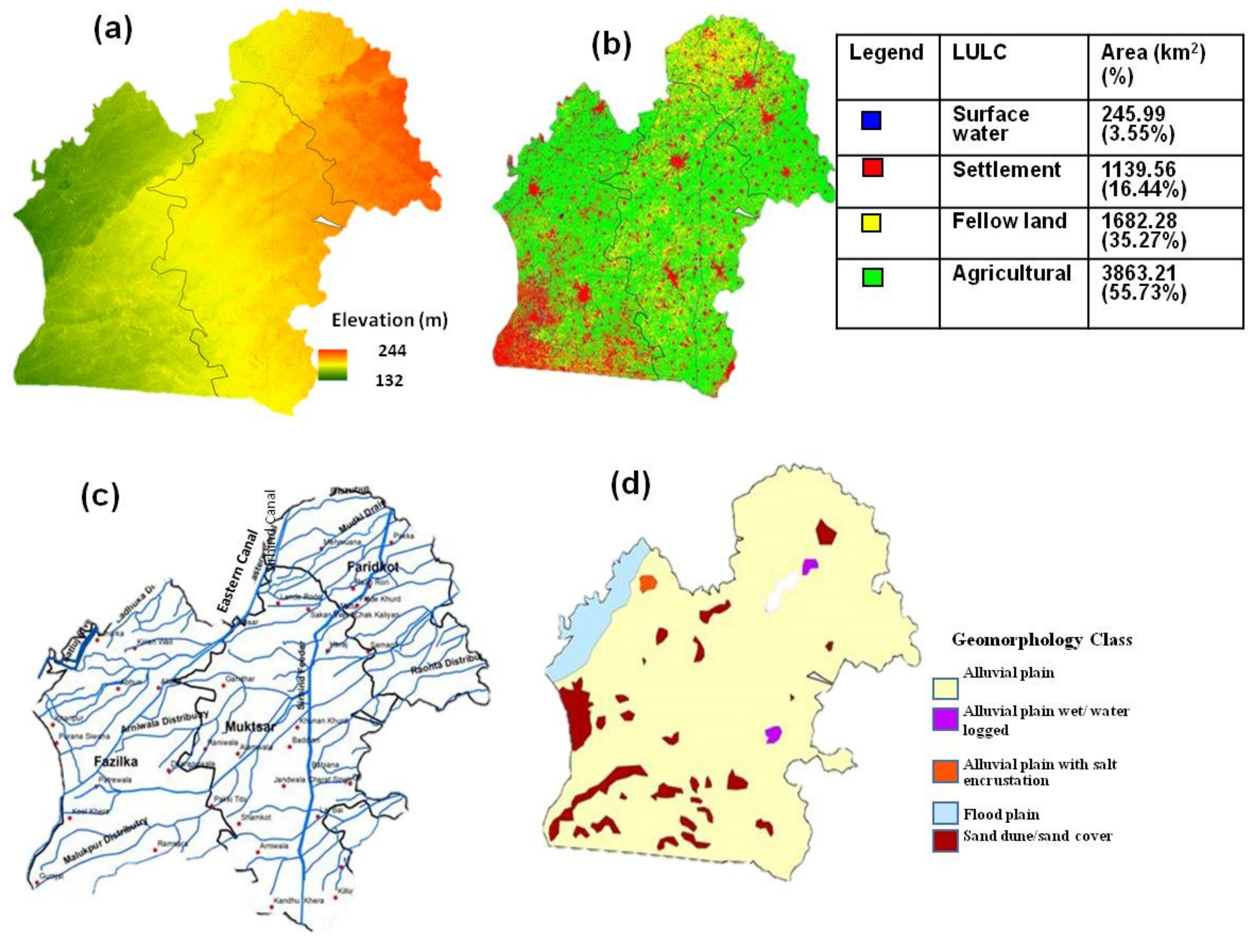
3.1. Surface Topography

A digital elevation model (DEM) is prepared with 30 m resolution (1-arcsecond) SRTM data (Figure 5a) to map the elevation and slope features (shows elevation variation) in the range from 132 m to 244 m, having a general topographic slope largely in the east–west direction. The ground elevation varies between 132 m above sea level (m asl) and 244 m asl in the study zone.

3.2. Land Use and Land Cover

A land use and land cover (LULC) map has been prepared using the Sentinel 2 multi-spectral imaging mission, showing habitat settlements, agricultural land (56%), fallow land (24%), forest, and water bodies (20%), as shown in Figure 5b. Results reveal that agriculture takes up a large share of the study area and requires high water demand, resulting in an increase in salinity.

3.3. Geomorphology and Surface Soil Features

A major part of the study area in the Sutlej Basin is occupied by alluvial plains. Further area is formed by the deposition of sediments with a low-lying flat topography. Some portions on the western side are flood plains, and some isolated patches of sand dunes are also found. Geomorphology of the study area is shown in Figure 5c. Soils are loamy, sandy desert soils and sodic and saline soils. The salt-affected soils identified in the study area are: soils with slight to moderate salinity and sodicity mostly on the surface; soils with slight salinity and sodicity throughout the soil profile; soils with moderate to high sodicity in the sub-soil; and soils with moderate salinity and strong sodicity on the surface and in the subsoil.

3.4. Drainage

The drainage system comprises a dense network of canals, as shown in Figure 5d. The water from these canals (Sirhind Feeder, Bikaner Canal, Rajasthan Feeder, Bathinda and Abohar branches of Sirhind Canal) is mainly used for irrigation purposes and has been fulfilling the irrigation demands of farmers for a long time. Similarly, there are large water bodies near the towns of Panjgrain, Khara, Jaito Mandi, Faridkot, and Wara Daraka that generally get dry in the summer.

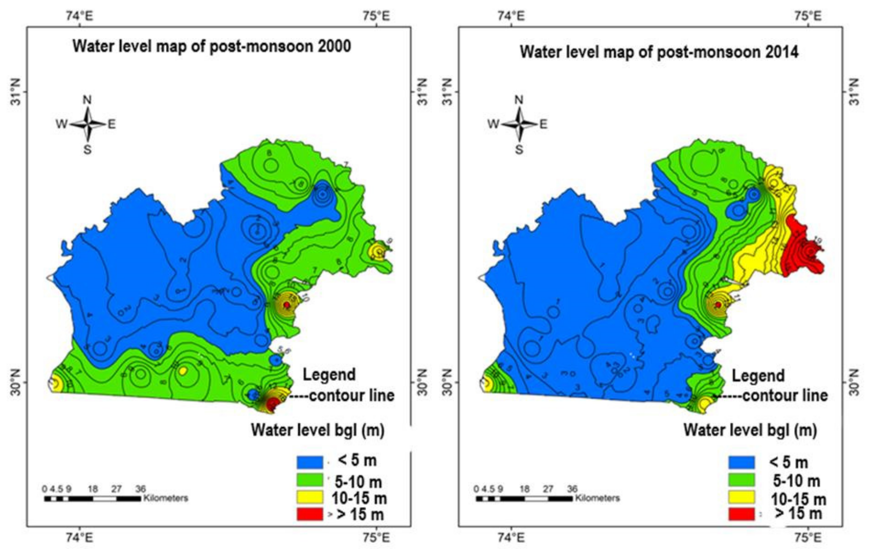
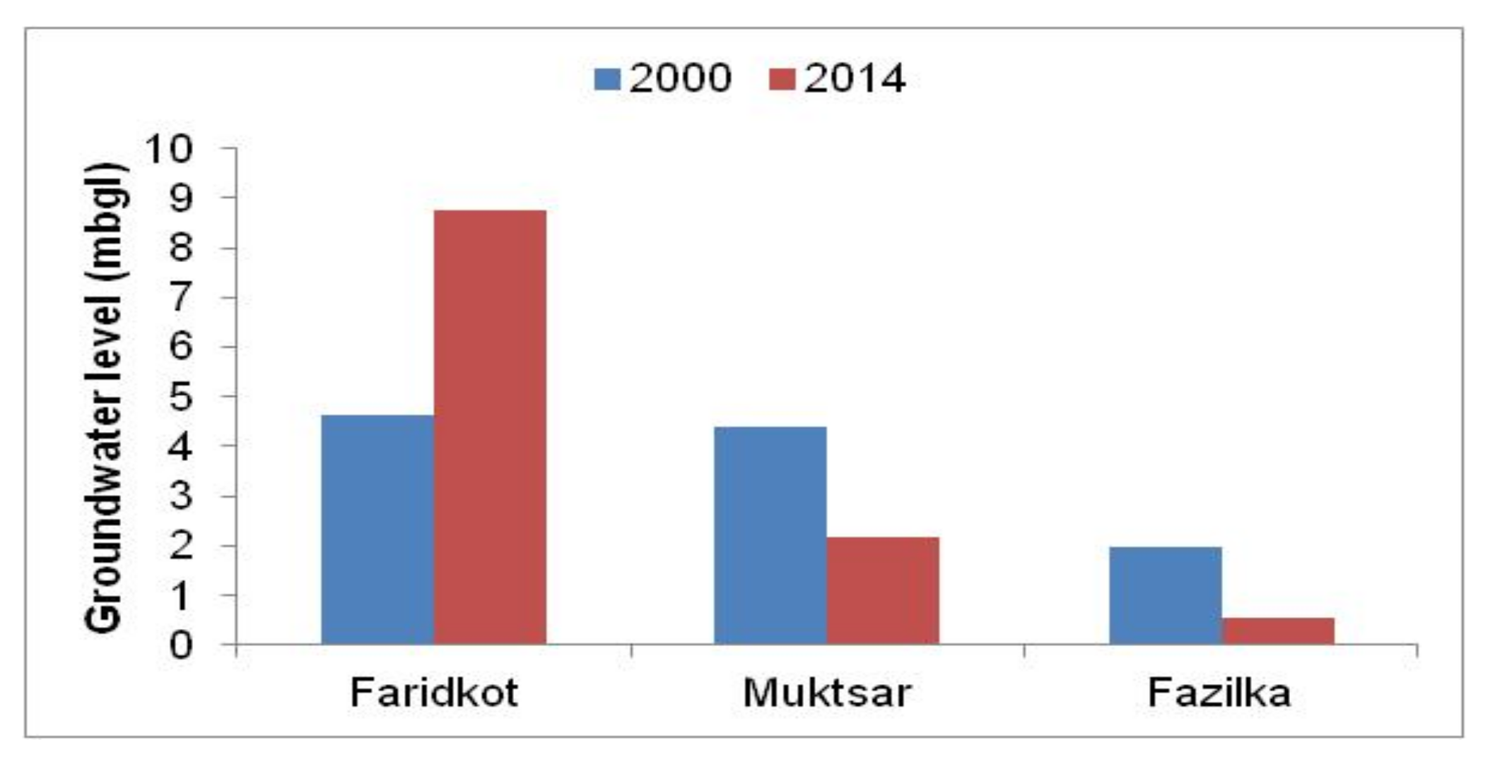
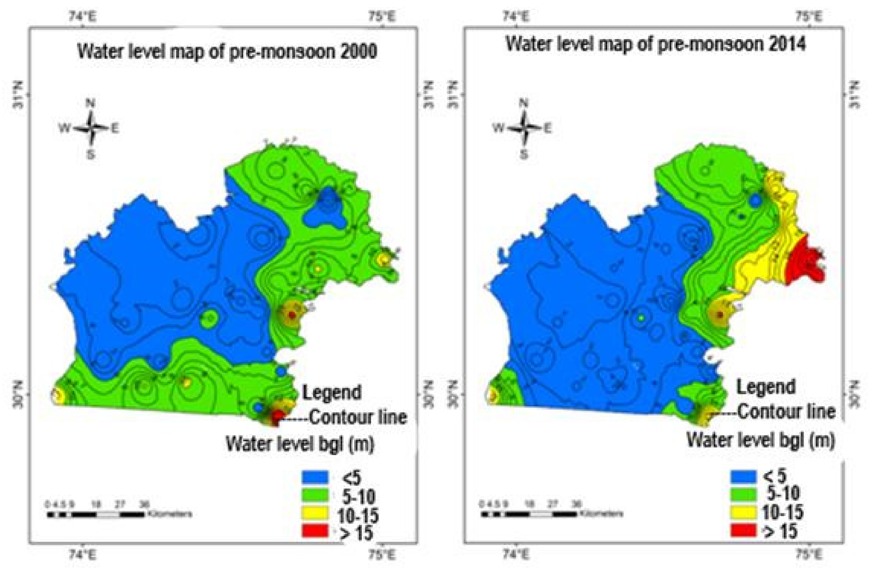
3.5. Groundwater Level Variations

The temporal variation of groundwater levels monitored in the three districts of the study area in the years 2000 and 2014 was analyzed to infer the groundwater fluctuation. In the total study area, the groundwater level varied between 0.20 and 27.40 m-bgl (168.45 to 220.45 m asl). It is inferred that there is a notable increase of 1–2 m in the groundwater levels in the Fazilka and Muktsar districts, while the groundwater levels decreased in the Faridkot district by an average of about 4 m (Figure 6). The variation in groundwater levels (2000 and 2014) shown for pre-monsoon and post-monsoon seasons are shown in Figure 7 and Figure 8, respectively.

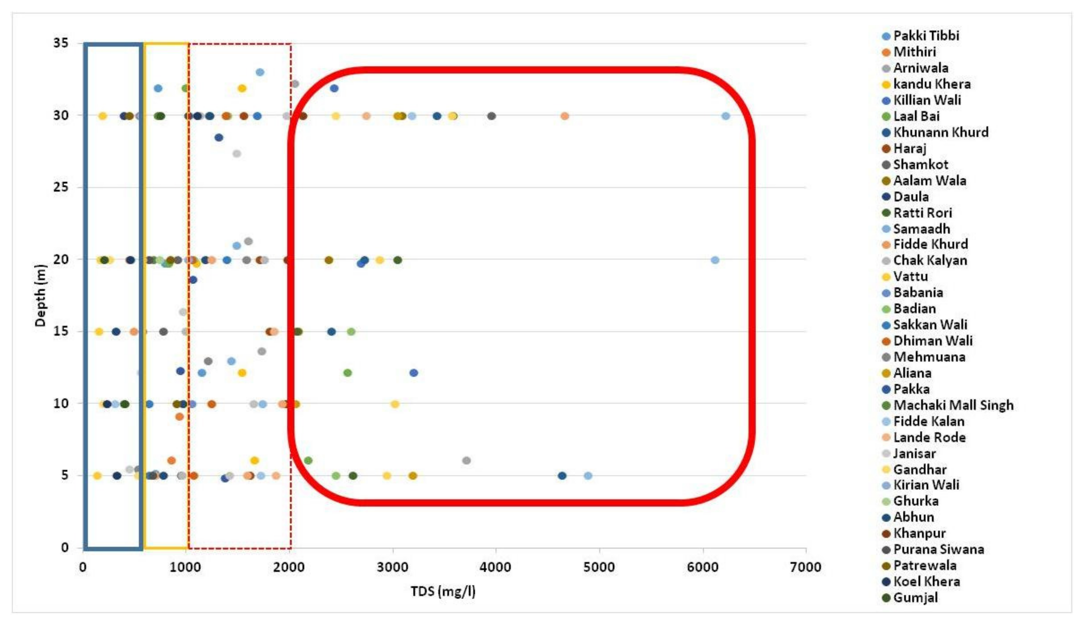
3.6. Spatial and Depth-Wise Salinity Variations

In the present study, salinity has been measured for all 142 piezometers at different depths, and location details are given in Figure 4. Groundwater salinity variation with depth, as shown in Figure 9, indicates that higher salinities are observed at depths 5–10 m and >20 m. The majority (>70%) of the water samples have salinity >1000 mg/L, and out of these, >32% of water samples have salinity greater than the drinking water permissible limit of 2000 mg/L. However, as discussed earlier, these values vary with aquifer depth and location of the piezometer.

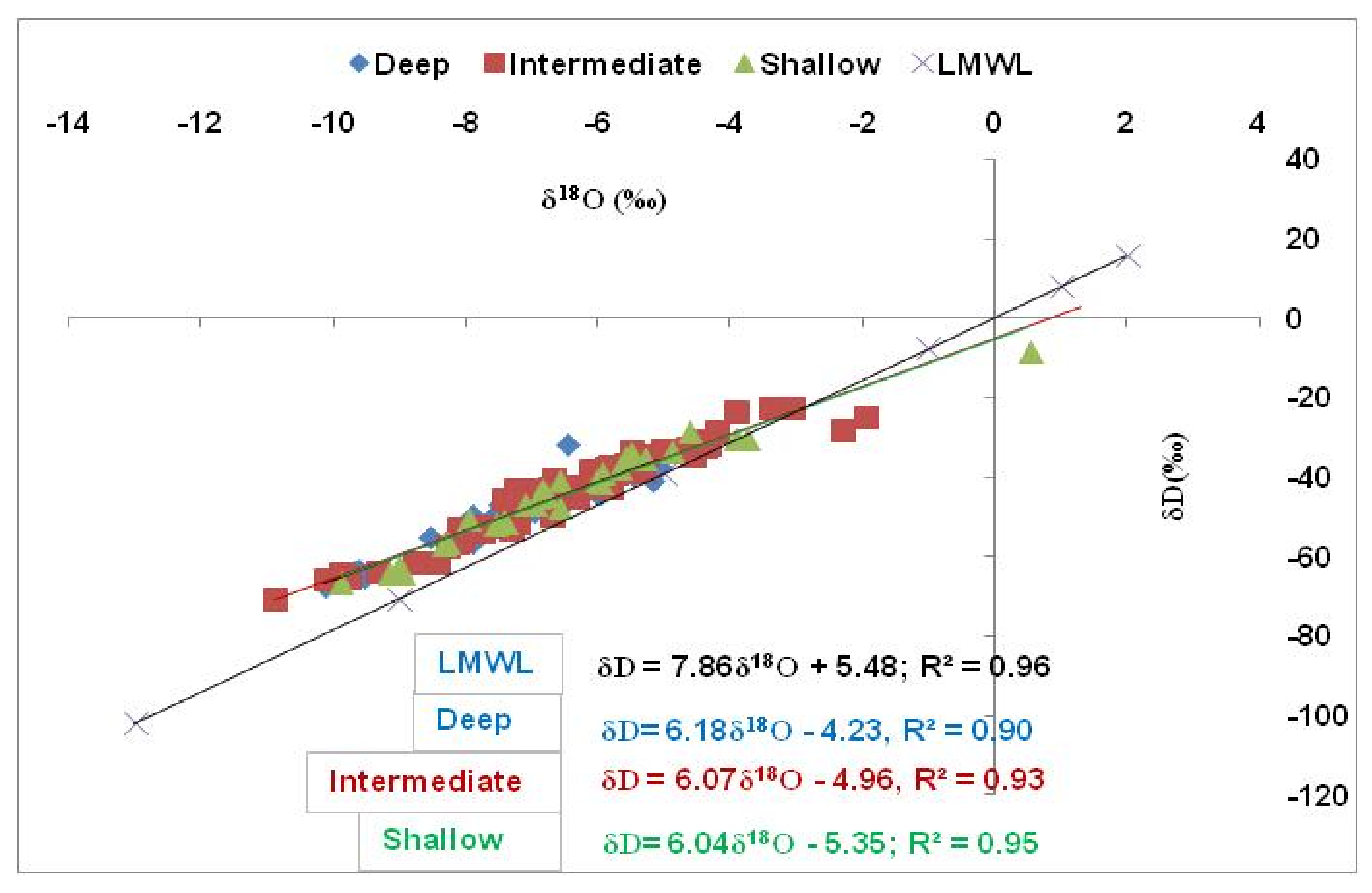
3.7. Isotope Database of Groundwater and Its Analysis

Isotopes have been used effectively in hydrological studies for providing vital information in a wide range of studies related to soil moisture variation; its movement and recharge through unsaturated zones; origin, age, and distribution of waters in a region including an occurrence and recharge mechanism; inter-connections between groundwater bodies and identification of recharge sources and areas; and investigation of groundwater contamination, including salinization, etc. [38]. Variations in the values of stable isotopes of water (δ¹⁸O and δD) result from isotope fractionation occurring under equilibrium and non-equilibrium conditions during both physical and chemical processes. Condensation is predominantly an equilibrium process, whereas evaporation occurs under non-equilibrium conditions [39].

Variations in stable isotope characteristics of groundwater are generally found due to different sources of recharge and their relative proportions. Therefore, if there is any change in the stable isotope composition of groundwater, it will reflect the same in recharge conditions (recharge zone and recharging source) and vice versa. This technique can be effectively used in conditions where there are alternating layers of freshwater and saline water in aquifers [6,11,19].

In the study, stable isotopes for identifying isotopic characteristics are employed in a cross plot between stable oxygen and hydrogen values, shown in Figure 10. The characteristic equations and the data range are given in

Table 1. Stable isotope composition of groundwater of districts Fazilka, Faridkot, and Muktsar.

Source	Equation (Calculated from Monthly Weighted Average)	Range (δ18O; δD)
GMWL (Rozanski et al., 1993)	δD = 8.17 δ18O + 10.35	--
Precipitation (Dolbaha) (Krishan et al., 2021)	δD = 7.9 δ18O + 5.48; R2 = 0.96; n = 322	10.9, −15; 67.5, −117.3
River Sutlej (Krishan et al., 2021)	δD = 7.2 δ18O + 0.16; R2 = 0.96; n = 51	0.15, −12.6; −18.6, −90.7
Canal (Krishan et al., 2021)	δD = 6.8 δ18O + 0.38; R2 = 0.97;	−6.06, −10.9; −42.7, −74.5
Groundwater (Deep ~30 m)	δD = 6.2 δ18O − 4.2; R2 = 0.90; n = 142	−5.09, −10.1; −31.9, −67.6
Groundwater (Intermediate 10–20 m)	δD = 6.1 δ18O − 5.0; R2 = 0.93; n = 142	−1.3, −10.9; −22.6, −71
Groundwater (Shallow ~<10 m)	δD = 6.0 δ18O − 5.4; R2 = 0.95; n = 142	0.5, −9.9; −8.9, −66.6

, and for the study area, these are provided by Krishan et al., [21]. Stable isotope data given in Figure 10 and Table 1 show that groundwater lines (for different depths) falls below the river Sutlej/canal and rainfall isotopic lines, indicating possibilities of groundwater recharge from canals. For more detailed analysis, depth-wise spatial distribution maps of stable isotopes were plotted.

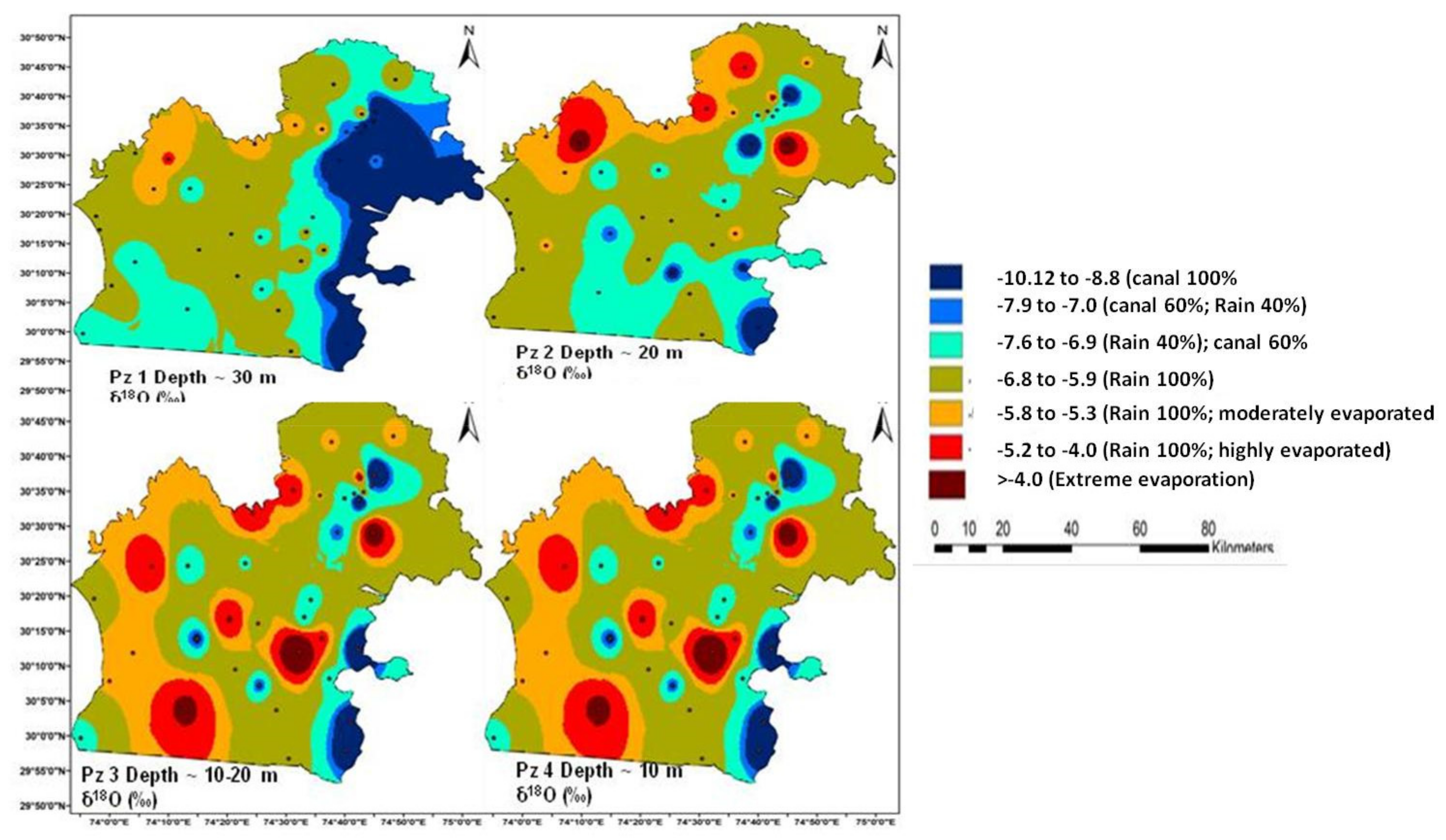
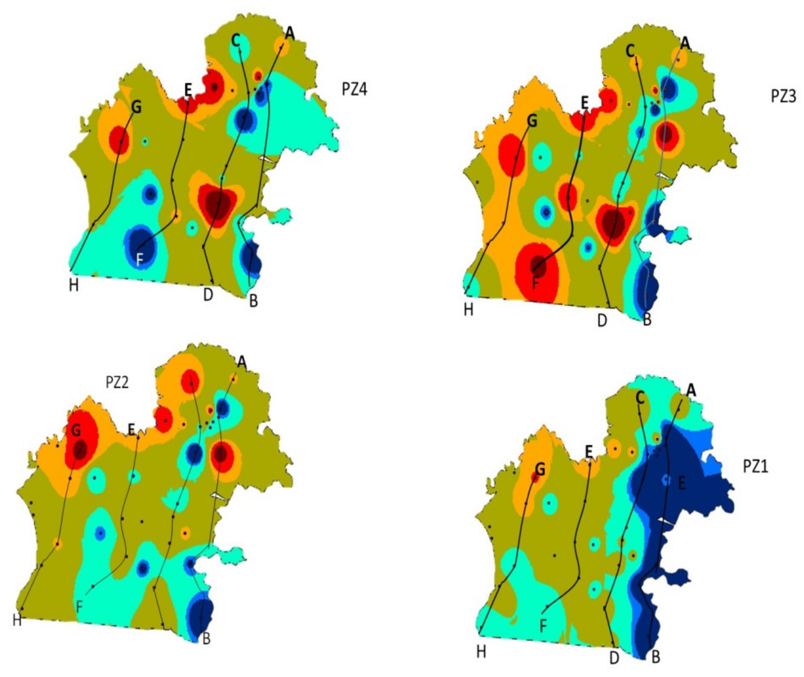
3.7.1. Spatial Distribution of Isotope Values of Groundwater

To investigate the source of water recharging the groundwater, spatial distribution patterns of groundwater samples collected from four depths, viz. PZ1 (~30 m), PZ2 (~20 m), PZ3 (~10 m), and PZ4 (5 m), were analyzed and interpreted. Assuming that the groundwater is formed due to recharge from a combination of canal water and rainwater and that, in some locations, evaporation affects rainwater, the spatial distribution stable isotopic maps prepared for different depth aquifers were divided into seven sub-categories according to the type of recharge water: (i) 100% recharge from the canal, (ii) recharge from canal and rain in a 60:40 ratio, (iii) recharge from canal and rain in a 40:60 ratio, (iv) 100% recharge from rain (without any substantial evaporation before recharge), (v) recharge from rainwater subjected to moderate level of evaporation, (vi) recharge of highly evaporated rainwater, and (vii) recharge of extremely highly evaporated rainwater. Maps prepared as per these seven sub-categories for four different groundwater depths (PZ1 to PZ4) are shown in Figure 11.

The recharging areal extent of recharge contributed by different recharge sources (as classified into seven sub-categories) to a depth of up to 30 m is estimated using GIS tools (

Table 2. Depth-wise recharge source area covered in the study area.

Groundwater Recharge Source (Code: Canal (C); Rain (R))	Isotopic Range (‰)	Aquifer Area Covered (%) at Different Depths
		PZ4 (<5 m)	PZ3 (~10 m)	PZ2 (~20 m)	PZ1 (~30 m)
C (100%)	−10.12 to −8.8	18.96	2.33	3.13	3.68
C (60%) + Rain (40%)	−7.9 to −7.0	4.83	1.78	1.59	2.68
R (60%) + C (40%)	−6.6 to −6.9	26.47	21.82	11.18	27.11
R (100%)	−6.8 to −5.9	43.01	55.23	49.31	51.41
Moderately evaporated rain water	−5.8 to −5.3	6.56	12.88	22.02	9.24
Highly evaporated rain water	−5.2 to −4.0	0.17	5.13	10.59	4.47
Extremely highly evaporated rain water	>−4.0	0.00	0.84	2.17	1.41

). Source-wise, the contribution of different recharging sources in recharging the groundwater (up to an aquifer depth of 30 m) comes out to be in the decreasing order of rain (~49.7%) > rain + canal in a 60:40 ratio (~21.6%) > moderately evaporated rainwater (12.7%) > canal (7%) > highly evaporated rainwater (5%) > canal + rain in a 60:40 ratio (2.7%). Overall, 82.7% of groundwater is formed from rain and the remaining 17.3% from canal water.

The isotopic comparison of the inter-aquifer groundwater system (PZ1 to PZ4) indicates both common and dissimilar features depending on the region of observation. The entire eastern part of the deep groundwater (PZ1) shows the canal as the major recharge source, but the immediate overlying aquifer (PZ2) does not show this feature. A large area falling in the southwest zone of the shallow aquifer (PZ4) shows groundwater of canal origin, but the immediate underlying aquifer (PZ3) shows its groundwater as being formed from partially evaporated rainwater. Groundwater in PZ3 shows a much larger portion of partially evaporated rainwater as its source of origin compared to the other overlying and underlying aquifers.

These dissimilarities indicate the origin of groundwater of these aquifers from the particular region lying outside the study area. Some common features that can be seen between these aquifers are that groundwater in the southeastern zone shows the canal as the source of recharge at all depths, and groundwater in the northern zone shows evaporated rainwater as the source of recharge in aquifers at all depths. These characteristics indicate vertical transmittance of groundwater from shallow to deep aquifers due to their unconfined conditions.

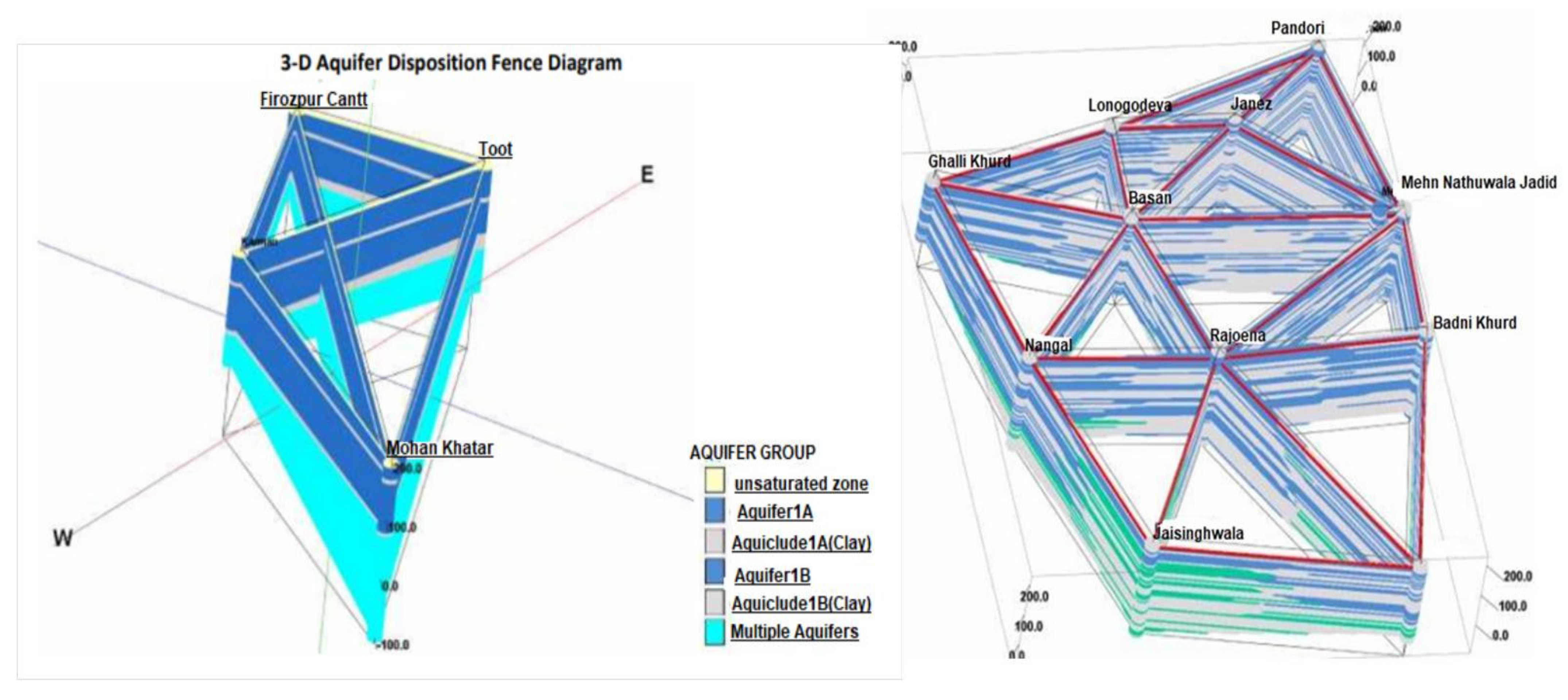
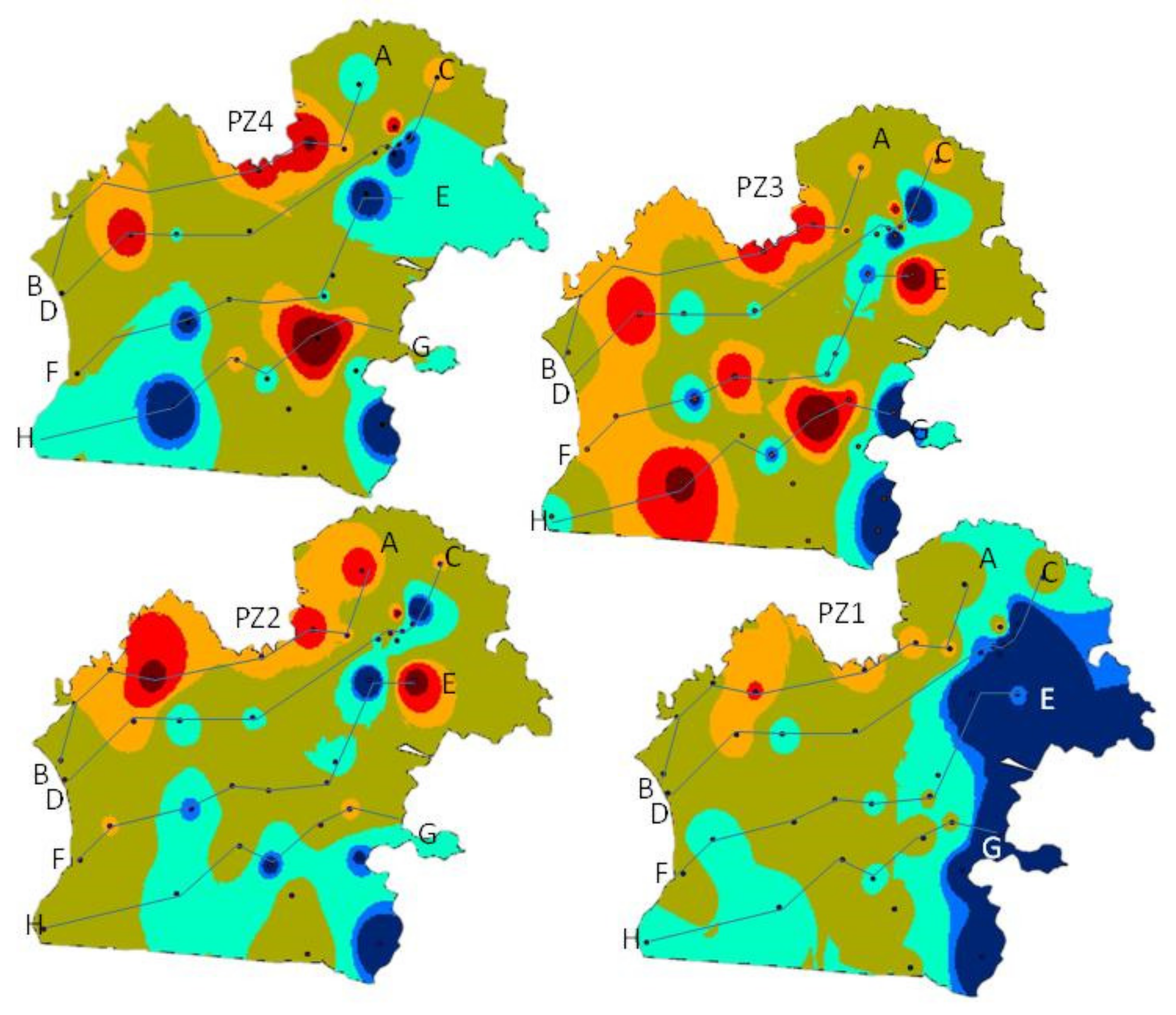
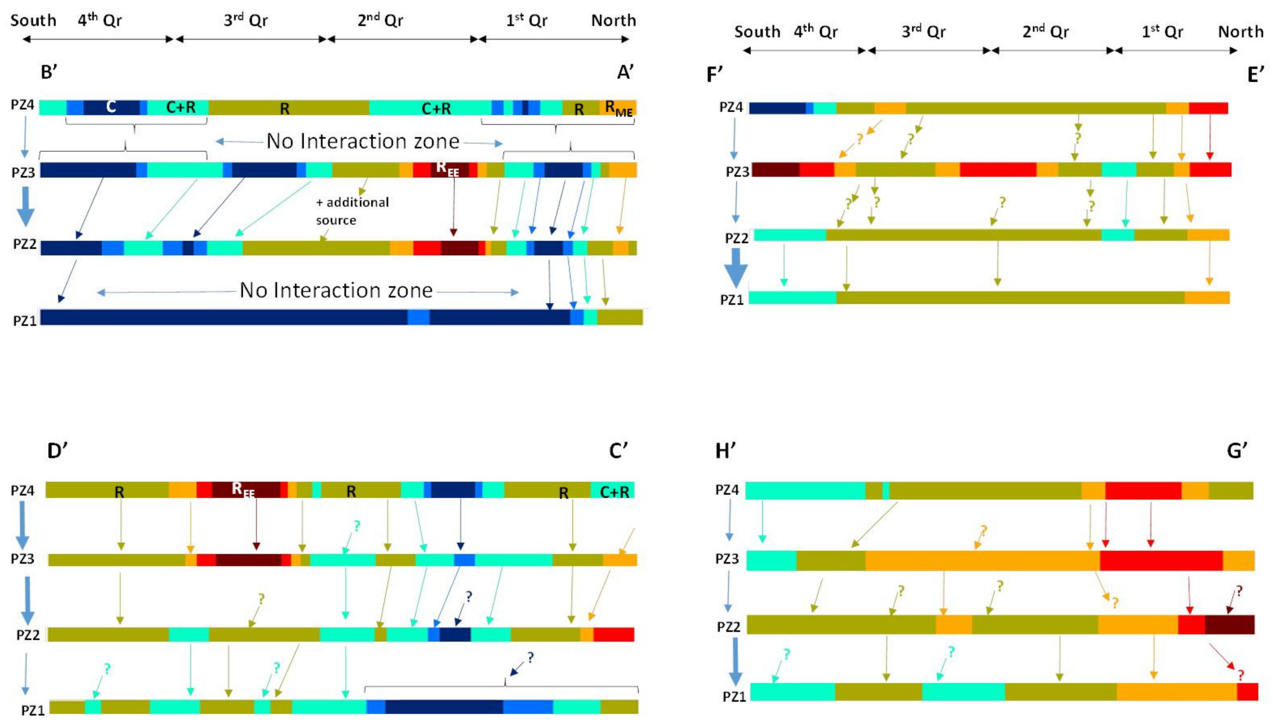
3.7.2. Isotope Data Interpretation for Aquifer Interaction Studies

In order to examine the interaction between the aquifers, the isotopic composition of groundwater between the underlying and overlying aquifers is inter-compared at the piezometric depths PZ1, PZ2, PZ3 and PZ4. The inter-comparison was done along four NE–SW-trending cross-sectional lines (AB, CD, EF, and GH). These lines are taken in the direction parallel to the topographic slope. Similarly, isotopic inter-comparison was done along four N–S trending cross-sectional lines (A’B’, C’D’, E’F’, and G’H’). All these lines were drawn carefully to see that they connect the maximum number of observation locations to make the data evaluation more closely resemble the observed data, as well as to minimize the interpolated region. The NE–SW- and N–S-trending lines at four depths are shown in Figure 12 and Figure 13. Each of these lines was then sub-divided into approximately 30 cells of size ~2.5 km × 2.5 km, and the isotopic values of these cells were read. Isotopic values of groundwater along these eight lines (AB, CD, EF, GH, A’B’, C’D’, E’F’, and G’H’) at the four piezometric depths (PZ1, PZ2, PZ3, and PZ4) were then inter-compared. The observed inter-comparison is shown in Figure 14, Figure 15 and Figure 16. The inter-comparison is interpreted based on the following parameters:

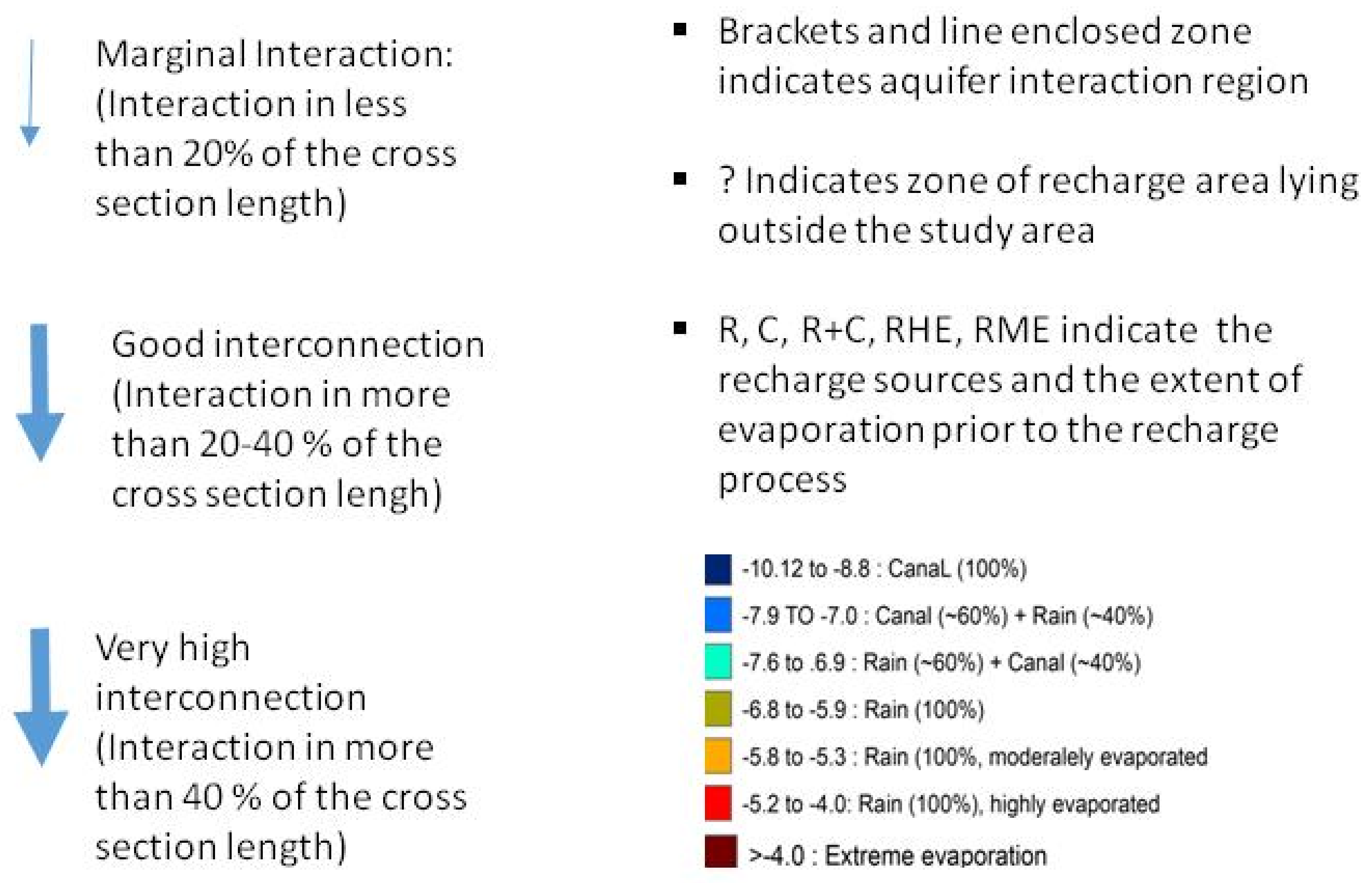
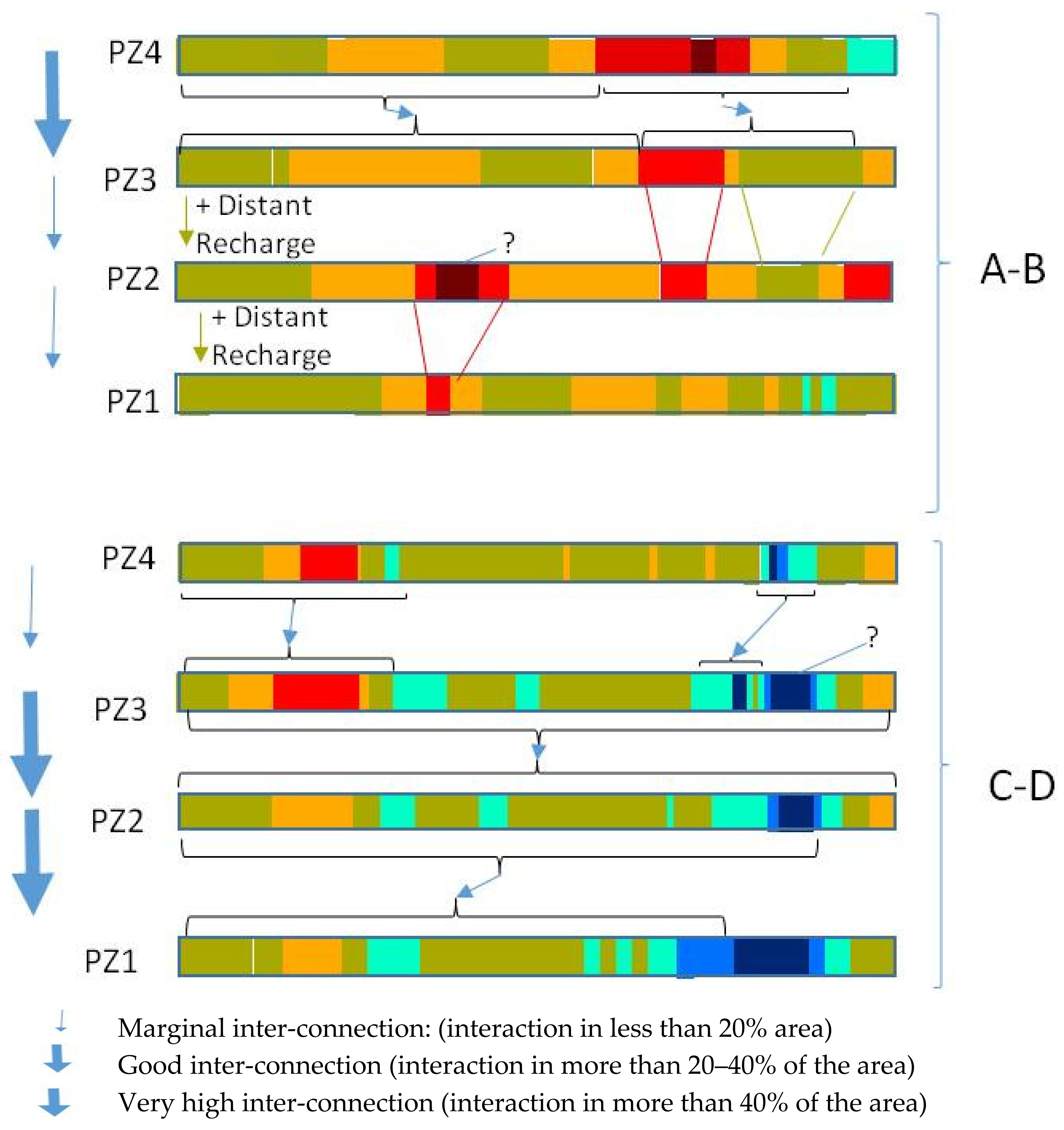
• On the basis of isotopic composition of groundwater, the source of recharge to the groundwater is designated as (i) canal (100%), (ii) canal (60%) + rain (40%), (iii) canal (40%) + rain (60%), (iv) rain (100%), (v) moderately evaporated rain, (vi) highly evaporated rain water, and (vii) extremely evaporated rain water.
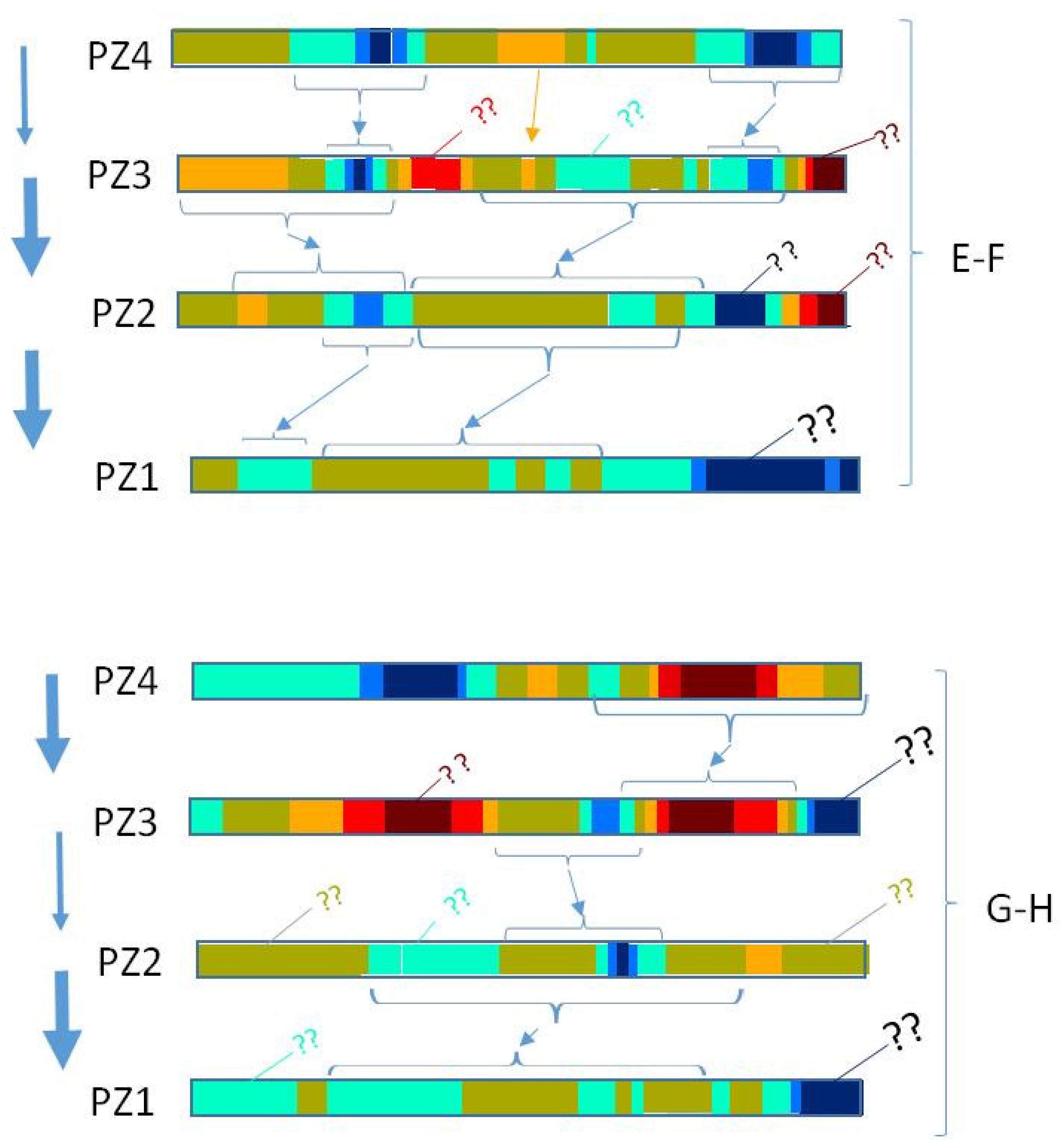
• A similar isotopic composition of groundwater in the overlying and underlying aquifers indicates the recharge of the underlying aquifer from the overlying aquifer, indicating a semi-confined condition between them (in Figure 14, Figure 15 and Figure 16, the recharge from the overlying aquifer is shown by arrow marks).
• Non-similarity in the isotopic composition of groundwater in the overlying and underlying aquifers indicates that the recharging sources of the overlying and underlying aquifers are different (indicating a confined condition of the underlying aquifer). In Figure 14, Figure 15 and Figure 16, non-interconnectivity is shown by the “?” mark. This means that the underlying aquifer is getting recharged from areas lying outside the study area.
• The aquifers are considered to be marginally interactive if the commonality in isotopic signatures of the overlying and underlying aquifers is not more than 20% of the cross-sectional length.
• Interaction between the overlying and underlying aquifers is considered to be good if, isotopically, groundwater between these aquifers shows common signatures over 20% to 40% of the cross-sectional length.
• The underlying aquifer is considered to be recharging largely from the overlying aquifer if the isotopic signatures of the overlying and underlying aquifers are similar over more than 40% of the cross-section length.

Using the above six points, the recharge sources (rain, canal water, and their combination) and the level of interaction between the overlying and underlying aquifers is interpreted and is presented in Figure 14, Figure 15 and Figure 16 and

Table 3. Groundwater flow between the aquifers (inter-aquifer interaction) along the cross-sections A–B, C–D, E–F and G–H.

Cross Section	Aquifer	Level of Inter-Connectivity in the Segment Zones 1 to 4
		1	2	3	4
A–B	PZ4 to PZ3	Moderate	Nil	Nil	Moderate
	PZ3 to PZ2	Very Good	Moderate	Low	Moderate
	PZ2 to PZ1	Low	Nil	Nil	Very low
C–D	PZ4 to PZ3	Low	Moderate	Good	Very good
	PZ3 to PZ2	Moderate	Good	Nil	Very good
	PZ2 to PZ1	Nil	Low	Low	Moderate
E–F	PZ4 to PZ3	Good	Nil	Nil	Nil
	PZ3 to PZ2	Moderate	Very low	Very low	Very low
	PZ2 to PZ1	Moderate	Very good	Very good	Very good
G–H	PZ4 to PZ3	Moderate	Very low	Nil	Moderate
	PZ3 to PZ2	Very low	Very low	Moderate	Moderate
	PZ2 to PZ1	Moderate	Good	Low	Very low

The extent of interaction is divided into 5 groups as (i) very low, (ii) low, (iii) moderate, (iv) good, and (v) very good. For convenience, the cross-section length is divided into 4 segments (1–4), as shown in Figure 16.

.

On the basis of color codes (similar isotopic value), correlation between the overlying and underlying aquifers is examined. A positive correlation indicates an interaction between the two aquifers (due to leakage or water exchange during irrigation activities). In the case that the underlying aquifer has different color code (isotopic value), then this indicates no recharge from the overlying aquifer. On this basis, the extent of interaction along all 32 cross sections was examined.

Regions with common isotopic signatures were considered a zone of interaction between the overlying and the underlying aquifers. Based on the extent of interaction, the aquifers along the cross-sections were demarcated as: (i) marginal inter-connection zones (interaction in less than 20% of the area), (ii) good inter-connection zones (interaction in more than 20–40% of the area), and (iii) very high inter-connection zones (interaction in more than 40% of the area).

Salinity in groundwater arises from the combination of evaporation enrichment and salt dissolution. The dissolved salts may be acquired from the salts of aquifer materials or the salts of surface soils that have dissolved and leached down with the recharging water. The process of salinity in groundwater may be checked by correlating the EC and stable isotopic maps. The zone of interaction between the aquifers can be effectively used in groundwater augmentation, management, and contamination control. The zone of interaction in the present study is mapped using stable isotopic composition.

In Figure 16, the color band represents the isotopic range (indicating the source water type) of the groundwater at that location and depth. Arrows between the aquifers indicate possible interconnectivity between the aquifers (due to similarity in their isotopic composition). The “?” indicates that the source water is not arising from the overlying aquifer, but rather as inflow from an area falling outside the cross-section zone. The resolution of the color band (minimum width in km that corresponds to a color line in the color band) is ~1 km.

For Figure 14, Figure 15 and Figure 16, an explanation of the symbols and text is given in Figure 17:

The temporal variation of groundwater levels monitored in three districts in 2000 and 2014 showed that the groundwater level varies between 0.20 and 27.40 m-bgl (168.45 to 220.45 m asl). It has been found that groundwater samples from about 31% of piezometers are marginally saline to saline (>2450 µS/cm). The isotopic comparison of the inter-aquifer groundwater system (PZ1 to PZ4) indicates both common and dissimilar features depending on the region of observation. These features are discussed as follows: The entire eastern part of the deep groundwater (PZ1) shows the canal as the major recharge source. However, the immediate overlying aquifer (PZ2) does not show this feature. A large area falling in the southwest zone of the shallow aquifer (PZ3) shows groundwater of canal origin, but the immediate underlying aquifer (PZ4) shows its groundwater as being formed from partially evaporated rainwater. Groundwater in PZ3 shows a much larger extent of evaporated rainwater as its source of origin compared to the other overlying and underlying aquifers.

The characteristics indicate vertical transmittance of groundwater from shallow to deep aquifers due to two unconfined conditions [39]. Firstly, groundwater in the southeastern zone shows the canal as the source of recharge at all depths. Secondly, groundwater in the northern zone shows evaporated rainwater in aquifers at all depths. Interactions between aquifers were assessed based on the isotope values, and it was found that regions with common isotopic signatures were considered zones of interaction between the overlying and the underlying aquifers [40,41]. Based on the extent of the interaction, the aquifers along the cross-sections were demarcated into three categories: (i) marginal inter-connection zones (interaction in less than 20% area), (ii) good inter-connection zones (interaction in more than 20–40% of the area), and (iii) very high inter-connection zones (interaction in more than 40% of the area).

4. Conclusions

On the basis of long-term groundwater fluctuations, areas are identified where groundwater may enter into the high-risk (dark) zone in the next 20 years, which needs urgent attention. From this study, the following suggestive measures can be provided for these areas: (i) where groundwater is getting recharged (or in identified recharge zones) on the basis of isotope analysis, these zones should be preferred for artificial recharge measures, and (ii) where canals are significant contributors to the groundwater, there is a need to maintain clean canal water so that interaction helps increase fresh groundwater resources. Low-water-intensive crops should be suggested in such areas.

There is a need to identify the sites where groundwater is picking up additional salinity when it is passing through. There is also an immediate need to install observation stations to monitor groundwater quality and levels at vulnerable locations, especially in fringe areas, where on one side groundwater quality is good, and immediately on the other side it deteriorates; areas where groundwater levels are becoming shallow and waterlogging may therefore occur; and areas where groundwater is deepening that may become dark zones. However, the conclusion drawn needs to be substantiated by groundwater age dating or any other suitable technique before field implementation. There is a need for detailed study to find out the sources of salinity and possible remedial measures.

References

1. Bonsor, H.C.; MacDonald, A.M.; Ahmed, K.M.; Burgess, W.G.; Basharat, M.; Calow, R.C.; Dixit, A.; Foster, S.S.D.; Gopal, K.; Lapworth, D.J.; et al. Hydrogeological typologies of the Indo-Gangetic basin alluvial aquifer, South Asia. Hydrogeol. J. 2017, 25, 1377–1406. [Google Scholar] [CrossRef] [Green Version]
2. Rodell, M.; Velicogna, I.; Famiglietti, J.S. Satellite-based estimates of groundwater depletion in India. Nature 2009, 460, 999–1002. [Google Scholar] [CrossRef] [PubMed] [Green Version]
3. NASA. Study: Third of Big Groundwater Basins in Distress. 2015. Available online: https://www.nasa.gov/jpl/grace/study-third-of-big-groundwater-basins-in-distress (accessed on 27 December 2020).
4. MacDonald, A.M.; Bonsor, H.C.; Ahmed, K.M.; Burgess, W.G.; Basharat, M.; Calow, R.C.; Dixit, A.; Foster, S.S.; Gopal, K.; Lapworth, D.J.; et al. Groundwater depletion and quality in the Indo-Gangetic basin mapped from in situ observations. Nat. Geosci. 2016, 9, 762–766. [Google Scholar] [CrossRef]
5. Custodio, E. Coastal aquifer salinization as a consequence of aridity: The case of Amurga phonolitic massif, Gran Canaria Island, in Study and Modelling of Saltwater Intrusion. In Proceedings of the 12th Saltwater Intrusion Meeting, Barcelona, Spain, First Week of November 1992; pp. 81–98. [Google Scholar]
6. Krishan, G.; Ghosh, N.C.; Kumar, C.P.; Sharma, M.; Yadav, L.; Kansal, M.L.; Singh, S.; Verma, S.K.; Prasad, G. Understanding stable isotope systematics of salinity affected groundwater in Mewat, Haryana, India. J. Earth Syst. Sci. 2020, 129, 109. [Google Scholar] [CrossRef]
7. Gopinath, S.; Srinivasamoorthy, K.; Saravanan, K.; Prakash, R. Tracing groundwater salinization using geochemical and isotopic signature in Southeastern coastal Tamilnadu, India. Chemosphere 2019, 236, 124305. [Google Scholar] [CrossRef]
8. Bennetts, D.A.; Webb, J.A.; Stone, D.J.M.; Hill, D.M. Understanding the salinisation process for groundwater in an area of south-eastern Australia, using hydrochemical and isotopic evidence. J. Hydrol. 2006, 323, 178–192. [Google Scholar] [CrossRef]
9. Jouzel, J.; Delaygue, G.; Landais, A.; Masson-Delmotte, V.; Risi, C.; Vimeux, F. Water isotopes as tools to document oceanic sources of precipitation. Water Resour. Res. 2013, 49, 7469–7486. [Google Scholar] [CrossRef]
10. Argamasilla, M.; Barber’a, J.A.; Andreo, B. Factors controlling groundwater salinization and hydrogeochemical processes in coastal aquifers from southern Spain. Sci. Total Environ. 2017, 580, 50–68. [Google Scholar] [CrossRef]
11. Krishan, G.; Prasad, G.; Kumar, C.P.; Patidar, N.; Yadav, B.K.; Kansal, M.L.; Singh, S.; Sharma, L.M.; Bradley, A.; Verma, S.K. Identifying the seasonal variability in source of groundwater salinization using deuterium excess—A case study from Mewat, Haryana, India. J. Hydrol. Reg. Stud. 2020, 31, 100724. [Google Scholar] [CrossRef]
12. Appelo, C.; Postma, D. Geochemistry, Groundwater and Pollution, 2nd ed.; Balkema: Rotterdam, The Netherlands, 2005. [Google Scholar] [CrossRef]
13. Adimalla, N. Groundwater Quality for Drinking and Irrigation Purposes and Potential Health Risks Assessment: A Case Study from Semi-Arid Region of South India. Expo. Health 2019, 11, 109–123. [Google Scholar] [CrossRef]
14. Singh, S.; Kumar, A.; Gupta, H. Activated banana peel carbon: A potential adsorbent for Rhodamine B decontamination from aqueous system. Appl. Water Sci. 2020, 10, 185. [Google Scholar] [CrossRef]
15. Kumar, A.; Jigyasu, D.K.; Subrahmanyam, G.; Mondal, R.; Shabnam, A.A.; Cabral-Pinto, M.M.S.; Malyan, S.K.; Chaturvedi, A.K.; Gupta, D.K.; Fagodiya, R.K.; et al. Nickel in terrestrial biota: Comprehensive review on contamination, toxicity, tolerance and its remediation approaches. Chemosphere 2021, 275, 129996. [Google Scholar] [CrossRef]
16. Kumar, A.; Pinto, M.C.; Candeias, C.; Dinis, P.A. Baseline maps of potentially toxic elements on soils of Garhwal Himalaya, India: Assessment of their eco-environmental and human health risks. Land Degrad. Dev. 2021, 32, 3856–3869. [Google Scholar] [CrossRef]
17. Houéménou, H.; Tweed, S.; Dobigny, G.; Mama, D.; Alassane, A.; Silmer, R.; Babic, M.; Ruy, S.; Chaigneau, A.; Gauthier, P.; et al. Degradation of groundwater quality in expanding cities in West Africa. A case study of the unregulated shallow aquifer in Cotonou. J. Hydrol. 2020, 582, 124438. [Google Scholar] [CrossRef]
18. Modibo Sidibé, A.; Lin, X.; Koné, S. Assessing Groundwater Mineralization Process, Quality, and Isotopic Recharge Origin in the Sahel Region in Africa. Water 2019, 11, 789. [Google Scholar] [CrossRef] [Green Version]
19. Krishan, G.; Sudersan, N.; Sidhu, B.S.; Vashisth, R. Impact of lockdown due to COVID 19 pandemic on Groundwater salinity in Punjab, India: Some hydrogeoethics issues. Sustain. Groundw. Resour. Manag. 2021, 7, 27. [Google Scholar] [CrossRef] [PubMed]
20. Krishan, G.; Taloor, A.K.; Sudarsan, N.; Bhattacharya, P.; Kumar, S.; Ghosh, N.C.; Singh, S.; Sharma, A.; Rao, M.S.; Mittal, S.; et al. Occurrences of potentially toxic trace metals in groundwater of the state of Punjab in northern India. Groundw. Sustain. Dev. 2021, 15, 100655. [Google Scholar] [CrossRef]
21. Krishan, G.; Kumar, B.; Sudarsan, N.; Rao, M.S.; Ghosh, N.C.; Taloor, A.K.; Bhattacharya, P.; Singh, S.; Kumar, C.P.; Sharma, A.; et al. Isotopes (δ18O, δD and 3H) variations in groundwater with emphasis on salinization in the State of Punjab, India. Sci. Total Environ. 2021, 789, 148051. [Google Scholar] [CrossRef]
22. Krishan, G.; Vashisth, R.; Sudersan, N.; Rao, M.S. Groundwater salinity and isotope characterization: A case study from south-west Punjab, India. Environ. Earth Sci. 2021, 80, 169. [Google Scholar] [CrossRef]
23. Yehdeghoa, B.; Rozanski, K.; Zojer, H.; Stichler, W. Interaction of dredging lakes with the adjacent groundwater field: An isotope study. J. Hydrol. 1997, 192, 247–270. [Google Scholar] [CrossRef]
24. Wang, W.; Yi, Y.; Zhong, J.; Kumar, A.; Li, S.L. Carbon biogeochemical processes in a subtropical karst river–reservoir system. J. Hydrol. 2020, 591, 125590. [Google Scholar] [CrossRef]
25. Bhat, M.A.; Zhong, J.; Dar, T.; Kumar, A.; Li, S.L. Spatial distribution of stable isotopes in surface water on the upper Indus River basin (UIRB): Implications for moisture source and paleoelevation reconstruction. Appl. Geochem. 2022, 136, 105137. [Google Scholar] [CrossRef]
26. Kumar, R.; Rani, M.; Gupta, H.; Gupta, B.; Park, D.; Jeon, B.H. Distribution of trace elements in flowing surface waters: Effect of seasons and anthropogenic practices in India. Int. J. Environ. Anal. Chem. 2017, 97, 637–656. [Google Scholar] [CrossRef]
27. Dansgaard, W. Stable isotopes in precipitation. Tellus 1994, 16, 436–468. [Google Scholar]
28. Zhu, L.; Fan, M.; Hough, B.; Li, L. Spatiotemporal distribution of river water stable isotope compositions and variability of lapse rate in the central Rocky Mountains: Controlling factors and implications for paleoelevation reconstruction. Earth Planet. Sci. Lett. 2018, 496, 215–226. [Google Scholar] [CrossRef]
29. Nayak, P.C.; Kumar, S.V.; Rao, P.R.; Vijay, T. Recharge source identification using isotope analysis and groundwater flow modeling for Puri city in India. Appl. Water Sci. 2017, 7, 3583–3598. [Google Scholar] [CrossRef] [Green Version]
30. Ahmed, I.M.; Jalludin, M.; Razack, M. Hydrochemical and Isotopic Assessment of Groundwater in the Goda Mountains Range System. Republic of Djibouti (Horn of Africa). Water 2020, 12, 2004. [Google Scholar] [CrossRef]
31. CENSUS. 2011. Available online: http://www.census2011.co.in/census/district/226-mewat.html (accessed on 13 January 2021).
32. CGWB. Aquifer Mapping and Management Plan, North Western Region. Central Groundwater Board, Ministry of Water Resources; Government of India: Chandigarh, India, 2017.
33. CGWB, Goverment of India. Groundwater Resources of Punjab State—As on 31st March, 2017—Prepared by CGWB-NWR and Water Resources and Environment Directorate; Government of Punjab: Punjab, India, 2018; p. 176.
34. APHA. Standard Methods for the Examination of Water and Waste Water, 22nd ed.; American Public Health Association: Washington, DC, USA; American Water Works Association: Denver, CO, USA; Water Environment Federation: Virginia, VA, USA, 2012. [Google Scholar]
35. Kumar, A.; Taxak, A.K.; Mishra, S.; Pandey, R. Long term trend analysis and suitability of water quality of River Ganga at Himalayan hills of Uttarakhand, India. Environ. Technol. Innov. 2021, 22, 101405. [Google Scholar] [CrossRef]
36. Van Weert, F.; Van der Gun, J.; Reckman, J. Global Overview of Saline Groundwater Occurrence and Genesis; IGRAC: Utrecht, The Netherlands, 2009. [Google Scholar]
37. IS: 10500; Specifications for Drinking Water. Bureau of Indian Standards: New Delhi, India, 2012.
38. Krishan, G.; Rao, M.S. Isotope Hydrology; Lambert Publishing House: Saarbrücken, Germany, 2013; p. 513. [Google Scholar]
39. Lapworth, D.J.; Krishan, G.; MacDonald, A.M.; Rao, M.S. Groundwater quality in the alluvial aquifer system of northwest India: New evidence of the extent of anthropogenic and geogenic contamination. Sci. Total Environ. 2017, 599, 1433–1444. [Google Scholar] [CrossRef] [Green Version]
40. Carol, E.; Kruse, E.; Mas-Pla, J. Hydrochemical and isotopical evidence of ground water salinization processes on the coastal plain of Samborombón Bay, Argentina. J. Hydrol. 2009, 365, 335–345. [Google Scholar] [CrossRef]
41. Gibbs, R.J. Mechanisms controlling world water chemistry. Science 1970, 170, 1088–1090. [Google Scholar] [CrossRef] [PubMed]
Figure 1. Study area map showing three districts in Punjab under study.
Water 14 00133 g001
Figure 2. Rainfall variation during the period of 1900–2019 in Fazilka, Muktsar, and Faridkot.
Water 14 00133 g002
Figure 3. Lithology of the study area [33].
Water 14 00133 g003
Figure 4. Piezometer development sites in the study area (Fazilka, Muktsar, and Faridkot).
Water 14 00133 g004
Figure 5. Important land surface features of the study area. Where (a) DEM of the study area (source: SRTM data); (b) LULC of Kharif season (source: SENTINEL-2, MSI data); (c) canal network: Eastern canal, Sirhind canal, and other minor canals in the study area; and (d) geomorphology.
Water 14 00133 g005
Figure 6. Water level variations (2000–2014) in Faridkot, Muktsar, and Fazilka.
Water 14 00133 g006
Figure 7. Water level map for pre-monsoon in Fazilka, Muktsar, and Faridkot.
Water 14 00133 g007
Figure 8. Water level map for post-monsoon in Fazilka, Muktsar, and Faridkot.
Water 14 00133 g008
Figure 9. Depth-wise salinity variations in piezometers in the study area.
Water 14 00133 g009
Figure 10. Cross plot (δ18O and δD) of groundwater samples in the study area.
Water 14 00133 g010
Figure 11. Spatial distribution of δ18O values of groundwater samples in the study area.
Water 14 00133 g011
Figure 12. Spatial distribution of δ18O values of groundwater samples in study area. Lateral cross sections, A–B, C–D, E–F, and G–H for mapping the inter-aquifer interaction.
Water 14 00133 g012
Figure 13. Vertical cross sections, A–B, C–D, E–F, and G–H for mapping the inter-aquifer interaction.
Water 14 00133 g013
Figure 14. Interactions in A–B and C–D cross-sections.
Water 14 00133 g014
Figure 15. Interactions in E–F and G–H cross-sections. Brackets and line enclosed zone indicates aquifer interaction region; ? (unknown) indicates zone of recharge area lying outside the study area. R, C, R + C, RHE, RME indicate the recharge sources as rain, canal, rain + canal, rain—highly evaporated water, and rain—moderately evaporated water, respectively, as well as the extent of evaporation prior to the recharge process.
Water 14 00133 g015
Figure 16. Water type and inter-aquifer interactions along the vertical cross-sections A’–B’, C’–D’, E’–F’, and G’–H.
Water 14 00133 g016
Figure 17. Explanation of the symbols and text in Figure 14, Figure 15 and Figure 16.
Water 14 00133 g017