Hybrid Fuzzy Multi-Criteria Analysis for Selecting Discrete Preferable Groundwater Recharge Sites

Abstract

This study proposes a hybrid fuzzy multi-criteria methodology for the selection of the most preferable site for applying managed aquifer recharge (MAR) systems by utilizing floodwaters. The use of MAR can increase water resources for later water utilization in case of drought. In this multi-criteria problem, seven recharge sites are under consideration, based on nine criteria, aiming to make a final list of their relative ranking. A fuzzy analytic hierarchy process (FAHP) based on the logarithmic fuzzy preference programming (LFFP) method is used to determine the weights of criteria. LFFP is an optimization-based method that produces a priority vector from a fuzzy pairwise comparison matrix. Furthermore, fuzzy inference systems (FIS) based on the Mamdani approach are used to estimate the rating of each alternative with respect to the criterion examined, and then the final evaluation of the alternatives is obtained. A FIS is a fuzzy if–then rule-based system where the experts’ qualitative knowledge is translated into numerical reasoning for each individual criterion. The proposed methodology is applied in the aquifer system of the agricultural plain located to the southeast of the city of Xanthi in the Prefecture of Xanthi, NE Greece.

1. Introduction

In recent decades, there has been growing concern about water availability, mainly due to the development of human societies and climate change [1]. Regarding the last one, trends show an increasing frequency and intensity of natural extreme events related to temperature and precipitation, such as droughts and floods [2,3,4,5].

A way of tackling low water availability challenges is the storage of water in artificial surface structures. However, this can meet only part of the increasing demand for water, mainly due to limited capacity, high evaporation losses, and competing objectives [6,7,8,9]. An alternative is groundwater recharge by utilizing excess surface water such as flood waters. Aquifers are more resistant to water supply variability related to drought than surface water supplies; however, they are under growing stress [6,10,11,12,13], especially in arid and semi-arid areas [14].

In recent years, managed aquifer recharge (MAR) systems have been increasingly used to increase groundwater availability for later use in dry seasons [15,16,17,18,19]. A variety of MAR techniques can be used that mainly depend on local conditions [20,21].

Scanlon et al. [12] state that two basic approaches for managing groundwater storage include: (1) conjunctive use (CU) of surface water and groundwater, and (2) managed aquifer recharge (MAR), which can be considered as an extension of CU. According to Foster and van Steenbergen [22], conjunctive groundwater use with surface water resources, in terms of practical water management, represents one of the most important responses to improving drought water supply security and for long-term climate change adaptation. Maliva [23] mentions that MAR can be viewed as a means for optimizing the use of aquifers. Dillon et al. [24] observed that the “objectives of groundwater management relate to maximizing economic utility of aquifers while sustaining the environment and providing security for meeting human needs”. Maliva [23] also states that depending upon the system, recharge is performed by either applying water onto a land surface (surface spreading), subsurface discharge into the vadose zone using wells, galleries, and trenches, or by injection using wells into either confined or unconfined aquifers. Particularly, surface spreading by using floodwater (excess winter water from a river) can be an effective MAR method [25]. A common technique for this method is the use of infiltration basins, while the suitability of an area for establishing floodwater spreading depends on various factors, such as geomorphology, hydrogeology, land use, socioeconomic issues, environmental impacts, etc., [26]. Recharge may also be induced by pumping groundwater close to connected surface water bodies (induced recharge). Modifications of the land surface and stream channels, such as by the removal (or change of) vegetation and construction of dams and levees, are also used to intentionally increase aquifer recharge.

A common issue that needs to be dealt with in applying MAR systems is the selection of suitable sites. Obviously, this is a problem of multi-criteria nature, in which an alternative or several alternative potential site/sites for applying MAR are considered based on a series of criteria, which may be divided into various categories. A variety of studies address this decision problem by the use of remote sensing and/or GIS techniques to produce a map with suitable zones for applying MAR (e.g., [27,28,29]). Other research provides advanced integrated methodologies by combining the GIS capabilities with multi-criteria methods (e.g., [30,31,32,33,34,35]). In such surveys, a weighted thematic layer for each criterion is produced. The criteria have been initially divided into classes (ranges) and each point of the grid obtains a score based on its classification into the classes. Then, a final map can be generated with overlay techniques using crisp operators of Boolean logic. Although these approaches are very significant and have been widely used, they are not always applicable. The main reason is the low data availability. The generation of thematic layers is based on interpolation methods, and therefore a small sample with respect to each criterion may diminish the reliability of interpolation results.

Fuzzy logic and fuzzy set theory were introduced by Zadeh [36] as a generalization of Aristotle’s logic and/or classical set theory. In Aristotle’s logic, a statement can be only true or false and, in classical set theory, an element x (or an individual) either belongs {1} or does not belong {0} to a given set and thus, it is described by two values [37]. In contrast to dual logic, fuzzy logic is many-valued and manipulates the concept of partial truth [38] and, in fuzzy set theory, an element x can partially participate in a (fuzzy) set, which means that it can obtain all the values in a closed unit interval [0, 1]. The principles of fuzzy logic and sets are the mathematical representation of human thinking and reasoning where truth may appear as an inference from inaccurate or partial knowledge, dealing with uncertainty due to vagueness. A variety of methodologies based on the principles of fuzzy logic and sets have been developed which incorporate the uncertainty of complex issues by the use of either autonomous fuzzy tools or hybrid analytical methods.

In particular, fuzzy logic and the theory of fuzzy sets have had an extensive use in hydrologic analysis and the analysis of hydrological multi-criteria problems since the early application of Bogardi et al. [39], in which fuzziness was used for partial satisfaction of objectives in regional water resources management, until the present [40]. The recent studies of Kazakis et al. [41], Kourgialas et al. [42], and Spiliotis et al. [43] are given as some examples of hybrid fuzzy multi-criteria methodologies. In these studies, the analysis can be carried out in order to either spatially address the examined multi-criteria problem, producing suitable fuzzy maps, or categorize points (alternatives) that can belong to several categories to some degree. This wide use of fuzzy logic and sets is due to the ability to simulate human reasoning in its use of approximate information, and to mathematize the uncertainty and vagueness in decision-making [44,45]. Furthermore, the use of fuzzy logic and sets in multi-criteria decision-making (MCDM) can express the gray zone of the decision and manage imprecise information (e.g., the score of criteria, the available resources), etc.

Regarding the selection problem of suitable recharge sites, most research uses fuzzy operators and/or fuzzy if–then rule-based systems in a GIS environment in order to produce a map with fuzzy suitable zones (e.g., [46,47,48,49,50,51,52]). However, the use of such models in combination with hybrid fuzzy multi-criteria methods to address this problem is an open issue.

The main proposal of this study is the ranking of seven alternatives representing suitable sites for applying MAR systems using floodwaters via a hybrid fuzzy multi-criteria methodology, in the context of increasing the local groundwater resources for later water use in case of drought. As described in the following section, the local conditions of the case study favor the application of floodwater spreading using infiltration basins. The evaluation of the alternatives was based on nine criteria that were selected based on the local conditions and the type of MAR. The weights of criteria were obtained through a fuzzy analytic hierarchy process (FAHP)-based methodology; however, they are crisp numbers. Fuzzy inference systems (FIS) were used in the rating of each alternative with respect to each criterion. The use of FIS was preferred since the objective function regarding the criteria was unknown. The composition of criteria was achieved through a simple aggregated model where a final ranking of the alternatives was obtained. The case study refers to the aquifer system of the agricultural plain located to the southeast of the city of Xanthi in northern Greece.

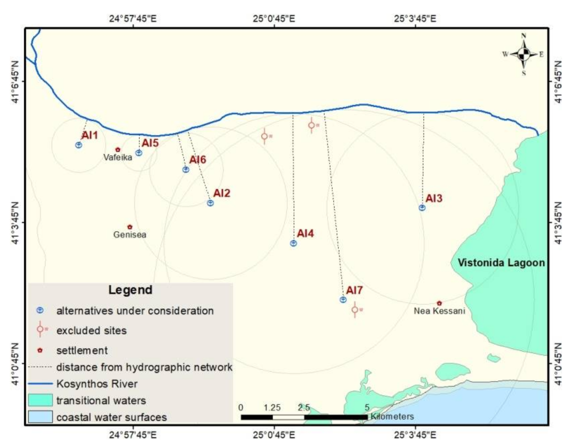
2. Case Study

The study area is the aquifer system of the agricultural plain located to the southeast of the city of Xanthi in the Prefecture of Xanthi, NE Greece (Figure 1). The wider region of study area is located within the boundaries of the tertiary Vistonida basin [53], while as presented in Figure 2 (modified map based on geological map of [54]), the aquifer system is hosted in the alluvial plain consisting of loam, clays, sands, gravels, etc. Gravels and sands of Pleiocene–Pleistocene origin occur in the north of study area, while Pleiocene brackish sediments, mainly consisting of sand and clay, with no wide surface spread, occur near Vistonida Lagoon. Clastic sediments of the Eocene and Oligocene, consisting of conglomerate breccia, limestones, and mollasic formations, occur in both the south and north of study area, while the background consists of igneous rocks that underlie andesitic rocks of the same geological period.

Geological formations of the alluvial plain range from fine to silty clay in the SE–E direction towards Vistonida Lagoon [53,55]. Regarding the geological structure and hydrogeological conditions, relevant assessments have shown that [56,57]:

(1)

Three main geological formations are presented: (a) the upper formation (8–80 m in thickness), of low permeability, consisting of clayey sand which interchanges at certain locations with gravel sand of little thickness, (b) the intermediate aquifer formation (10–70 in thickness), consisting of permeable gravel sand, considered as a shallow confined aquifer, in some locations changing to semi-confined aquifer, and (c) the lower impermeable formation consisting of clayey silt in depth of 30–90 m;

(2)

Transmissivity, T, ranges from 90 to 915 (m²/day), while the storage coefficient, S, ranges from 2.4 × 10⁻⁴ to 8.75 × 10⁻²;

(3)

The shallow aquifer system is naturally recharged, mainly from direct infiltration of precipitation and partially from percolation of the River Kosynthos (upstream zone of coarse-grained deposits);

(4)

The groundwater flow has a SE direction, being almost identical to that of the old riverbed’s direction in the area;

(5)

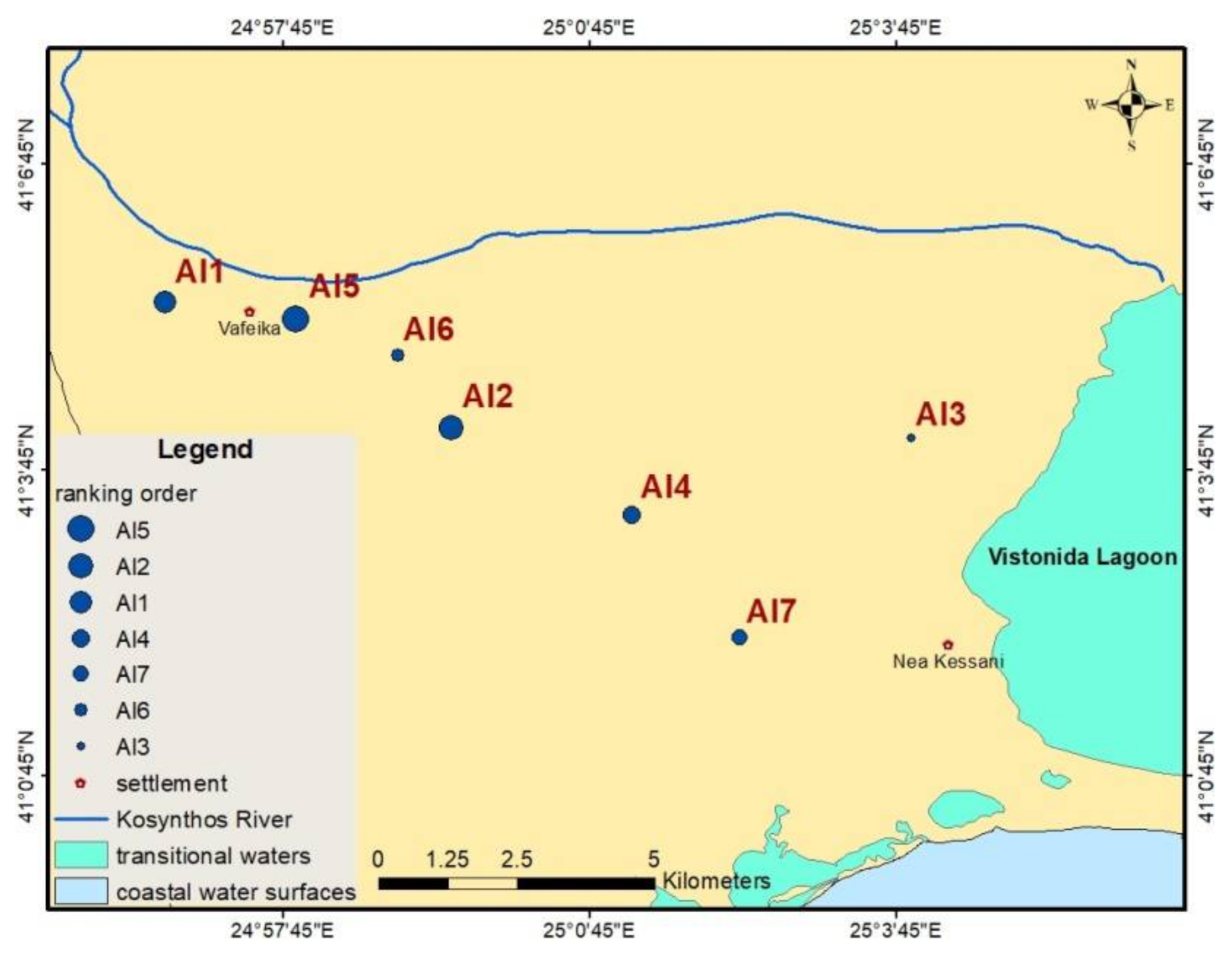
The groundwater main recharge axes appear to be in a S–SE direction towards Vistonida Lagoon;

(6)

The high quality of the water of the River Kosynthos gives rise to its use for artificial recharge purposes.

The climatic conditions of the wider area differ in the lowlands from those in the mountains [58]. Based on precipitation and temperature records from the meteorological station of Genisea (41°04′07′′ N–24°59′44′′ E) located in the study area, the mean annual cumulative precipitation is 605.6 mm in the period 1966–2018. The available temperature data concern the period of 1988–2018, in which the mean annual temperature was 14.4 °C, while mean temperature of the summer months was 23.9 °C. In the wider region, both wet periods (that caused flood events such as the flood of the Kosynthos River in 1996) and drought periods have occurred. In fact, a drought period might have had an effect on groundwater levels of the examined aquifer. Particularly, the groundwater level in January of the shallow aquifer is significantly related to drought in the previous hydrological year and drought in the first trimester of the current hydrological year [59].

The exploitation of the aquifer system mainly takes place in the south of the riverbed of the Kosynthos River where there is a significant number of irrigation wells. Most of these wells there are not deeper than 50 m, while there are a few shallow wells (up to 10 m) that are not in use any more [58,60]. According to Diamantis et al. [60], the annual pumping volume is estimated at 48 × 10⁶ m³ approximately. The spatial distribution of the irrigation wells and other detailed information regarding the study area can be found in the studies of Diamantis et al. [60] and Pisinaras [58].

3. Materials and Methods

The development of the proposed hybrid fuzzy methodology refers to the intermediate formation of the case study. It can only be applied in unconfined aquifers and where there is an underlying drainage axis. In addition, the application of the methodology requires the presence of an adjacent river whose excess water during the flood period can be utilized without burdening the ecological supply. Last, in order for each alternative to be evaluated, the lithological profile and hydraulic characteristics of both the vadose zone and saturated zone had to be available. Each alternative represents a potential site for MAR application where there is a well with available hydrogeological data. The alternatives were considered through the nine criteria described below in ascending order of importance. The selected criteria can be added or subtracted depending on the specific conditions of an area, while there is no limit in number of the examined alternatives.

3.1. Criteria Description

Ecological status (C₁): This refers to the status of the Kosynthos River. Based on River Basin Management Plans [61], the riverbed of Kosynthos is divided into sections characterized by different ecological status. Each alternative may be supplied water for applying MAR by a different section. The worst case is unknown ecological status, while the best case is high ecological status.

Slope (%) (C₂): Slope is a commonly-used criterion in identification of suitable sites for applying MAR. Obviously, the steeper the slope, the less desirableare conditions for applying MAR. The dividing of slope into classes is based on previous studies (e.g., [35,62]); however, the classes of slope were adjusted to the case study area, which is characterized by smooth slopes.

Distance from hydrographic network (m) (C₃): This refers to the distance between each alternative and a source with available water for MAR. Only the distance from the Kosynthos River was considered since the water of Vistonida Lagoon is unsuitable due to its connection with coastal water surfaces (Figure 3). In the research of Farhadian et al. [63], the distance from rivers is also used, while in other research (e.g., [35]) the distance from drainage networks is taken into account.

Distance from road network (m) (C₄): This criterion may affect the suitability of an area for applying MAR either in a negative or a positive way. For instance, it is desirable a recharge site is a minimum distance from highways and freeways in order for potential groundwater pollution to be avoided [52]. However, this holds in the case of short distance (a few hundred meters) between the recharge site under consideration (alternative) and the potential pollution source. On the other hand, if the distance between the alternatives and road network is in the order of kilometers, where there is in fact no danger of groundwater pollution, then an easy and fast access to the recharge site is desirable [63]. In this study, the distance of the alternatives from the highway was in the order of kilometers; therefore, the shorter distance, the higher the rating of the alternative. Figure 4 presents a map with the distances in kilometers of each alternative from the highway.

Transmissivity (m²/day) (C₅): This is a common hydrogeological parameter used in studies regarding the selection of suitable recharge sites [32,35,52,64], since it takes into account both the (horizontal) hydraulic conductivity (K) and the saturated thickness of the aquifer (b). High transmissivity values favor the recharge process since transmissivity (T) is defined as T = Kb (m²/day). According to Pisinaras [58], in the study area, T ranges between 25 and 2950 (m²/day).

Storativity (C₆): Another hydrogeological criterion used in site selection for applying MAR is storativity (S) [65]. The storativity of each alternative in the study area was obtained based on previous research [56,57,58], where storage coefficient values varied from 10⁻² to 10⁻⁴. The lower the S-values, the more unfavorable conditions are for applying MAR.

Hydraulic resistance (C₇): This is a critical hydrological criterion because in its calculation, $c={\displaystyle \sum _{i=1}^n}{d}_i/K_i$, the (vertical) hydraulic conductivity (K) (m/days) of each sedimentary layer and its thickness (d) (m) are introduced. Kazakis [35] suggests the use of (log values) hydraulic resistance to take into account the permeability of the entire thickness of the vadose zone. High c-values indicate unsuitable recharge sites. It is noted that in the case of confined aquifers, this criterion cannot be used. The estimation of c-values of the alternatives was based on the research of Pisinaras [58], in which stratigraphic columns regarding the examined alternatives are available.

Type of aquifer (C₈): As aforementioned, the hydraulic resistance does not refer to confined aquifers. Thus, the classes of this criterion are considered to be crisp. That is, an alternative has the highest rating (10) when its aquifer is unconfined (or/and leakage aquifer), otherwise it is zero. Based on the available stratigraphic columns [58], there were confined underlying aquifers in the cases of three alternatives and, thus, these alternatives were excluded from the analysis. The aquifers of the other seven alternatives were unconfined or/and leakage (semi-confined) aquifers.

Piezometry (C₉): Piezometry and the type of aquifer are essential (hydrogeological) criteria for applying MAR systems. When a recharge axis is underlying an alternative, then this recharge site is unsuitable and vice versa. The identification of the study area regarding the recharge axes and the drainage axes was based on previous research [56,57,58].

On that point, it should be noted that the proposed methodology has been developed in order to analyze both large and small datasets with various hydrogeological parameters. Hence, some parameters such as aquifer type (e.g., confined) have been included in order to help to this analysis. Initially, all available information (lithological profiles, hydraulic parameters, etc.) was selected, and after the first screening, the alternatives with no available profiles were eliminated and thus, ten alternatives remained. Based on the lithological profiles, three of ten alternatives overlie confined aquifers, and hence, these alternatives were excluded from the analysis (Figure 3 and Figure 4). On balance, the following preparatory steps were carried out (Figure 5):

(1)

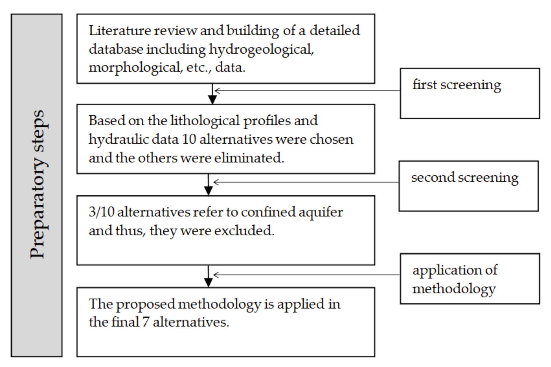
Literature review and building of a detailed database including hydrogeological, morphological, etc., data;

(2)

The points with lithological profiles and hydraulic data of the aquifer and vadose zone were chosen for the application and development of the methodology. The other sites were eliminated;

(3)

Tensites were then chosen, of which 3 referred to confined aquifers, and for this reason they were excluded from the analysis;

(4)

The method was applied to the final chosen sites (7 in total) and the most suitable for MAR application was determined.

Figure 5. Preparatory steps for screening of the final alternatives.

Figure 5. Preparatory steps for screening of the final alternatives.

3.2. Fuzzy Analytic Hierarchy Process—FAHP

As aforementioned, fuzzy logic has a wide use in multi-criteria analysis and has been applied to several hydrological issues. The basic concepts of fuzzy logic and sets, such as the membership function, α-cuts, fuzzy number [66], extension principle [67,68] and max–min composition of fuzzy relations [69], are presented in Appendix A. The fuzzy methods used in this study are based on these concepts.

One of the most used methods for quantification of the significance of criteria is the analytic hierarchy process (AHP) suggested by Saaty [70]. As is known, the AHP is based on pairwise comparisons between criteria (or/and alternatives), where a positive reciprocal pairwise comparison matrix ${\mathit{A}}_{\mathit{n}\mathit{x}\mathit{n}}$ is constructed. A fundamental scale is used [70] in order to numerically express the initial experts’ judgments regarding the relative criteria importance (ratios of weights $(w_i/w_j)$); however, it is not the only one [71]. Based on the eigenvalue theory from linear algebra, Saaty [70] developed the eigenvector method (EVM) in order to obtain a unique solution to derive the weights of criteria (or alternatives) from a ${\mathit{A}}_{\mathit{n}\mathit{x}\mathit{n}}$. This is the principal eigenvector w determined by solving the system of equations:

$$\left({\mathit{A}}_{\mathit{n}\mathit{x}\mathit{n}}-{\lambda }_{\max }\mathit{I}\right)\mathit{w}=0\iff {\mathit{A}}_{\mathit{n}\mathit{x}\mathit{n}}\mathit{w}={\lambda }_{\max }\mathit{w}$$

(1)

where I is the unit matrix and ${\lambda }_{\max }$ is the principle eigenvalue of ${\mathit{A}}_{\mathit{n}\mathit{x}\mathit{n}}$.

Given that the initial judgments cannot be identical to the ratios of weights, the ${\mathit{A}}_{\mathit{n}\mathit{x}\mathit{n}}$ is not fully consistent. Therefore, the validation of AHP is based on the measure of the consistency of the ${\mathit{A}}_{\mathit{n}\mathit{x}\mathit{n}}$. For this reason, the consistency index CI = (λ_max − n)/(n − 1) is estimated. Then, the CI-index is divided with a predefined index (RI), the value of which depends on the number of criteria n.

Fuzzy set theory is the most widely used approach integrated with the AHP [72]. The use of fuzziness can incorporate the inherent uncertainty in the assessments of pairwise comparison between criteria, derived by the subjectivity in the quantification of the ratios expressing the relative importance of the decision elements (weights of criteria and ratings/scores of alternatives).

To cope with the uncertainty of imprecise judgments, Chang [73] used a fuzzy pairwise comparison matrix and then he used extent analysis to extract a crisp priority vector. An advantage of the Chang method is its computational simplicity.

However, even if extent analysis has been widely used (e.g., [74,75,76,77]), it has a major drawback. This is the fact that a weight of a criterion may obtain zero value, and hence it makes no sense for such a criterion to be under consideration [78]. In addition, extent analysis produces a priority vector, which may be quite different from the true one, and thus the weights obtained are not representative regarding the relative importance of decision criteria.

Mikhailov [79], extending his previous research [80], suggests a method for derivation of crisp weights from a matrix with fuzzy judgments, by applying a fuzzy preference programming (FPP)-based nonlinear method (optimization approach). In fact, the method of Mikhailov [79] is based on (fuzzy) flexible programming; that is, the uncertainty appears in the constant term of the fuzzy constraints [68].

Let us consider the following reciprocal matrix ${\tilde{\mathit{A}}}_{\mathit{n}\mathit{x}\mathit{n}}$ with fuzzy pairwise comparisons between n criteria:

$$\tilde{A}={\left({\tilde{a}}_{ij}\right)}_{nxn}\begin{array}{cc}\begin{array}{ccccc}{C}_1\hspace{1em}\hspace{1em}\hspace{1em}& \hspace{1em}{C}_2\hspace{1em}\hspace{1em}& \hspace{1em}\hspace{1em}{C}_3\hspace{1em}\hspace{1em}& \hspace{1em}\dots & \hspace{1em}{C}_n\hspace{1em}\end{array}& \\ \left[\begin{array}{ccccc}1& \left(l_{12},m_{12},u_{12}\right)& \left(l_{13},m_{13},u_{13}\right)& \dots & \left(l_{1n},m_{1n},u_{1n}\right)\\ \left(l_{21},m_{21},u_{21}\right)& 1& \left(l_{23},m_{23},u_{23}\right)& \dots & \left(l_{2n},m_{2n},u_{2n}\right)\\ \left(l_{31},m_{31},u_{21}\right)& \left(l_{32},m_{32},u_{22}\right)& 1& \dots & \left(l_{3n},m_{3n},u_{3n}\right)\\ \dots & \dots & \dots & \dots & \dots \\ \left(l_{n1},m_{n1},u_{n1}\right)& \left(l_{n2},m_{n2},u_{n2}\right)& \left(l_{n2},m_{n2},u_{n2}\right)& \dots & 1\end{array}\right]& \begin{array}{c}\begin{array}{c}{C}_1\\ C_2\end{array}\\ C_3\\ \begin{array}{c}⋮\\ C_n\end{array}\end{array}\end{array}$$

(2)

where C_i (for i = 1, …, n) are the criteria, ${\tilde{a}}_{ij}=1/{\tilde{a}}_{ji}=w_i/w_j$, that is $l_{ij}=1/u_{ji}$, $m_{ij}=1/m_{ji}$ and $u_{ij}=1/l_{ji}$ for $l_{ij}\le m_{ij}\le u_{ji}$ and for all $i,j=1, 2,\dots ,n,\hspace{1em}j\ne i$.

In order to obtain crisp weights whose ratios are approximately included in the initial fuzzy judgments ($l_{ij}\tilde{\le }{w}_i/w_j\tilde{\le }{u}_{ij}$), the following membership function is introduced by Mikhailov [79]:

$${\mu }_{ij}\left(w_i/w_j\right)=\{\begin{array}{l}\frac{\left(w_i/w_j\right)-l_{ij}}{m_{ij}-l_{ij}},\hspace{1em}\hspace{1em}{l}_{ij}<\left(w_i/w_j\right)\le m_{ij}\\ \frac{u_{ij}-\left(w_i/w_j\right)}{u_{ij}-m_{ij}},\hspace{1em}\hspace{1em}{u}_{ij}>\left(w_i/w_j\right)\ge m_{ij}\end{array}$$

(3)

where ${\mu }_{ij}\left(w_i/w_j\right)$ denotes the degree of satisfaction (membership) to which the ratio $\left(w_i/w_j\right)$ belongs to fuzzy judgment ${\tilde{a}}_{ij}$.

In order to determine a global evaluation from individual membership functions [81], a proper fuzzy operator, that is the min intersection, is used with respect to the above fuzzy inequalities. The min intersection is preferred because it secures a common satisfaction of all the selected membership functions [82,83]. Furthermore, in this study, the use of min intersection can linearize the decision problem

$$\lambda =\min \left\{{\mu }_{ij}\left(w_i/w_j\right)|i=1,\dots ,n-1,j=i+1,\dots ,n\right\}$$

(4)

where λ is the degree of the common satisfaction to which the crisp priority vector satisfies simultaneously each fuzzy pairwise comparison.

Assuming that the decision-maker looks forward to the highest membership degree of the ratio of weights in the fuzzy judgments ${\tilde{a}}_{ij}$, Mikhailov [79] and Mikhailov and Tsvetinov [84] maximize λ under the constraint that the total sum of weights must be equal to the unit (normalization constraint) and the positivity constraint in their values:

$$\begin{array}{l}\max \lambda \\ s.t.\\ \{\begin{array}{l}\underset{ij}{\min }\left[{\mu }_{ij}\left(w_i/w_j\right)\right]\ge \lambda ,\hspace{1em}\hspace{1em}i=1,\dots ,n-1,\hspace{1em}\hspace{1em}j=i+1,\dots ,n\\ {\displaystyle \sum _{i=1}^n{w}_i=1}\\ w_i\ge 0,\hspace{1em}\hspace{1em}i=1,\dots ,n\end{array}\end{array}$$

(5)

In the case of a positive λ-value, all solution ratios completely satisfy the fuzzy judgments, while a negative λ-value indicates strongly inconsistent initial judgments [79].

This paper applies the logarithmic fuzzy preference programming (LFPP)-based methodology for fuzzy AHP priority derivation proposed by Wang and Chin [85].The LFPP-based nonlinear method is preferred over the FFP-based nonlinear method because (a) it can ensure nonnegative values of membership function and hence, it produces a unique optimal solution and, (b) the same priority vectors are derived; either the upper triangular elements of a fuzzy pairwise comparison matrix are used or the lower ones.

Wang and Chin [85] addressed the drawbacks of Mikhailov’s method [79]. Initially, they used logarithmed values in fuzzy judgments, which can be justified based on the extension principle, and the strict monotony of the (increasing) function $\ln {\tilde{a}}_{ij}$ [86]:

$$\ln {\tilde{a}}_{ij}\approx \left(\ln l_{ij}, \ln m_{ij}, \ln u_{ij}\right)$$

(6)

Equation (6) is an approximation of the fuzzy judgments $\ln {\tilde{a}}_{ij}$ considered as fuzzy triangular numbers, since due to the logarithmic transformation the linearity does not hold. The membership function ${\mu }_{ij}(\ln {\tilde{a}}_{ij})$ of the triangular fuzzy number can be expressed by the following Equation (7) [85].

$${\mu }_{ij}\left(\ln \left(w_i/w_j\right)\right)=\{\begin{array}{l}\frac{\ln \left(w_i/w_j\right)-\ln l_{ij}}{\ln m_{ij}-\ln l_{ij}},\hspace{1em}\hspace{1em}\ln \left(w_i/w_j\right)\le \ln m_{ij}\\ \frac{\ln u_{ij}-\ln \left(w_i/w_j\right)}{\ln u_{ij}-\ln m_{ij}},\hspace{1em}\hspace{1em}\ln \left(w_i/w_j\right)\ge \ln m_{ij}\end{array}$$

(7)

Following Mikhailov’s approach [79], it would be desirable to construct an optimization problem (Equation (8)) in which the parameter $\lambda =min\{{\mu }_{ij}\left(\ln \left(w_i/w_j\right)\right)$ for i = 1, …, n − 1 and j = i + 1, …, n to be maximized.

$$\{\begin{array}{l}\max \lambda \\ s.t.\hspace{1em}{\mu }_{ij}\left(\ln \left(w_i/w_j\right)\right)\ge \lambda \\ \hspace{1em}\hspace{1em}{w}_i\ge 0,\hspace{1em}i=1,\dots ,n\\ \hspace{1em}\end{array}\hspace{1em}\iff \hspace{1em}\{\begin{array}{l}\max \hspace{1em}1-\lambda \\ s.t.\hspace{1em}\ln w_i-\ln w_j-\lambda \left(\ln \left(m_{ij}/l_{ij}\right)\right)\ge \ln l_{ij}\\ \hspace{1em}\hspace{1em}\ln w_j-\ln w_i-\lambda \left(\ln \left(u_{ij}/m_{ij}\right)\right)\ge -\ln u_{ij}\\ \hspace{1em}\hspace{1em}{w}_i\ge 0,\hspace{1em}i=1,\dots ,n\end{array}$$

(8)

For simplicity reasons, in the above optimization problem, the normalization constraint might be carried out after the solution. Nevertheless, a negative λ-value can still occur, which means that the inequalities of Equation (8) do not simultaneously hold. In other words, there is no an optimal solution (priority vector) to satisfy all the fuzzy judgments at the same time. Thus, according to Wang and Chin [85], two nonnegative deviation variables, ${\delta }_{ij}$ and ${\eta }_{ij}$, are introduced whose values must obviously be minimum. Therefore, the optimization problem applied in this research takes the following form:

$$\begin{array}{c}\mathrm{Minimize} {(1-\lambda )}^2+M{{\displaystyle \sum }}_{i=1}^{n-1}{{\displaystyle \sum }}_{j=i+1}^n({\delta }_{ij}^2+n_{ij}^2)\hfill \\ s.t.\hfill \\ \hspace{1em}\hspace{1em}\hspace{1em}\hspace{1em}\hspace{1em}\hspace{1em}\hspace{1em}\left\{\begin{array}{c}{x}_i-x_j-\lambda \left(\ln \left(\frac{m_{ij}}{l_{ij}}\right)\right)+{\delta }_{ij}\ge ln{l}_{ij}, i=1,\dots ,n-1, j=i+1,\dots ,n\\ x_j-x_i-\lambda \left(\ln \left(\frac{u_{ij}}{m_{ij}}\right)\right)+n_{ij}\ge -ln{u}_{ij}, i=1,\dots ,n-1, j=i+1,\dots ,n\\ \lambda ,x_i\ge 0, i=1,\dots ,n-1, j=i+1,\dots ,n\end{array}\right.\end{array}$$

(9)

where M is a specific constant term aiming for nonnegativity of λ, and to hold the values of deviation variables low, $x_i=ln{w}_i,ln{w}_j=x_j$.

The nonlinear objective function of Equation (9) focuses on minimizing the deviation variables, and after the priorities’ derivation, the normalization of weights takes place (Equation (10)) in order to produce optimal normalized weight values.

$$w_i=\frac{\exp \left(x_i^{*}\right)}{{\displaystyle \sum _{j=1}^n\exp \left(x_j^{*}\right)}},\hspace{1em}i=1,\dots ,n$$

(10)

where $x_i^{*}(i=1,\dots ,n)$ is the optimal solution of Equation (9).

The uniqueness of the obtained optimal priority vector holds due to the convexity of the λ and the linearity of constraints. The other advantage of the LFFP based-nonlinear method (Equations (6)–(10)), which is the alignment of priorities regardless of the triangular part of the comparison matrix used, can be easily proved [85] after some simple algebraic transformation.

3.3. Fuzzy Inference Systems for the Evaluation of the Alternatives’ Rating

This research uses the fuzzy inference system (FIS) based on Mamdani’s approach [87] for the evaluation of the alternatives. In this study, the use of such a system was preferred because the function for the criteria synthesis was unknown. With the use of FIS, the ranges of criteria can be fuzzified as well. The input variable of the FIS was the examined criterion and the output variable was the rating of each alternative with respect to the examined criterion. Both the input and the output variables of the FIS were divided into classes (ranges), which were considered fuzzy sets (fuzzy trapezoidal numbers) and described by linguistic variables. Briefly, the linguistic variables (Figure 6) quantify the natural language characterizing the words by fuzzy sets defined in the universe of discourse in which the variable is defined [69]. Thus, each alternative, based on its numeric value regarding the examined criterion, takes a membership degree of belonging to each fuzzy class (range) of the criterion. The rating (R) of an alternative, concerning the examined criterion, depended on the activation degree of the fuzzy if–then rules designed by the experts. It is pointed out that a FIS was designed for each criterion that was examined.

The general structure of a FIS consists of the following components [88,89]:

(1)

A fuzzifier. The degree to which the input data (the numeric value of the alternative with respect the examined criterion) satisfy the fuzzy rule is calculated. In this step, the classes of the input variables (criteria) are fuzzified.

(2)

An inference engine module. A series of fuzzy if–then rules is modulated. Based on the satisfaction degree described in the previous step and the selected fuzzy implication, the fuzzy rules fire strength to infer knowledge. Thus, a fuzzy conclusion is calculated for each rule.

(3)

Aggregation. All fuzzy conclusions inferred by all fuzzy rules are combined into a final fuzzy conclusion.

(4)

A defuzzifier. The fuzzy output (inferred knowledge) is translated to crisp output (rating of each alternative with respect to the examined criterion).

From a mathematical point of view, a FIS, based on the Mamdani model, is composed of the premise (antecedent if–part) and conclusion (consequent then–part). It can be formulated as follows [82]:

$$Ru(k):If x_1 is A_1^k and x_2 is A_2^k\dots and x_z is A_z^k then y is B^k$$

(11)

where $A_z^k$ is a fuzzy set in Universe $U\subset \mathbb{R}$ (input variables of the model), $B^k$ is a fuzzy set in Universe $Z\subset \mathbb{R}$ (output variables of the model), ${(x_1,x_2,\dots ,x_z)}^T\in U$, $y\in Z$ and k is the fuzzy rule kth. The above linguistic rule describes a mapping from U₁ × U₂ × … × U_z to Z [88].

In this research, the antecedent of the fuzzy if–then rule includes only one input variable:

$$Ru(k): If x is A^k then y is B^k$$

(12)

The contribution of the rule kth, Ru(k), to the output (inferred conclusion) of the model is also a fuzzy set which may be represented by a fuzzy implication. Here, the common engineering fuzzy implications of the algebraic product (Equation (13)) and the min implication (Equation (14)) are used, which are suited to inference on the basis of phenomenological information [90,91]. The min fuzzy implication is recommended in the case that there is no distinction between cause and effect [90].

$${\mu }_{Ru{}^k}(x,y)={\mu }_{A^k}(x)\cdot {\mu }_{B{}^k}(y)$$

(13)

$${\mu }_{Ru{}^k}(x,y)=\min \left\{{\mu }_{A{}^k}(x), {\mu }_{B{}^k}(y)\right\}$$

(14)

Let a fuzzy rule consists of two fuzzy propositions as follows:

$$\begin{array}{l}Fuzzy proposition 1: x is A^{\prime }{}^k\\ Fuzzy proposition 2: Ru->If x is A{}^k then y is B{}^k\end{array}\}Conclusion: y is B^{\prime }{}^k$$

(15)

Then, according to the generalized modus ponens (GMP) concept [66], a new fuzzy proposition should be inferred such that the closer $A^{\prime }{}^k$ to $A^k$, the closer $B^{\prime }{}^k$ to $B^k$. Therefore, based on the concept of GMP, a fuzzy conclusion can be defined for each fuzzy rule with respect to the given input:

$${\mu }_{B^{\prime }{}^k}(y)=\underset{\mathrm{x}\in \mathrm{X}}{{\displaystyle \sup }} t \left[{\mu }_{A^{\prime }{}^k}(x), {\mu }_{R{u}^k}(x,y)\right]$$

(16)

Other t-norms, instead of the algebraic product, could be used (Equation (17)). The following Equation (17) is in fact a max–min composition in case the input is a vector. Practically, it holds:

$${\mu }_{B^{\prime }{}^k}(y)=\underset{\mathrm{x}\in \mathrm{X}}{{\displaystyle \max }}\hspace{1em}\left[{\mu }_{A^{\prime }{}^k}(x)\wedge {\mu }_{R{u}^k}(x,y)\right]={\mu }_{A^{\prime }{}^k\circ R{u}^k}(y)$$

(17)

In the case that the input data of the model are crisp numbers (fuzzy singleton), it holds:

$${\mu }_{A^{\prime }{}^k}(x)=\{\begin{array}{l}1\hspace{1em}if x=x*\\ 0 otherwise\end{array}$$

(18)

where x* is a point in its universe.

Consequently, based on the fuzzy implication process, a fuzzy conclusion corresponds to each fuzzy rule. In order to obtain a final fuzzy conclusion regarding the examined criterion, all the fuzzy conclusions must be combined. This procedure is called the aggregation process and is carried out by using an operator which, in this research, is the max union.

In conclusion, in a fuzzy inference system based on the Mamdani model, the fuzzy implication of algebraic product, the algebraic product for all t-norms, and the fuzzy max union are selected. In the case of crisp input data, the Mamdani’s product inference engine is described in Equation (19) [69]. In the case that the min fuzzy implication, min for all t-norm operators and the max union are selected, then the fuzzy output of the system is expressed by Equation (20).

$${\mu }_{B^{\prime }}(y)=\underset{k=1}{\overset{L}{{\displaystyle \max }}}\left[{\mu }_{A^k}(x_i*)\cdot {\mu }_{B^k}(y)\right]$$

(19)

$${\mu }_{B^{\prime }}(y)=\underset{k=1}{\overset{L}{{\displaystyle \max }}}\left[\min \left\{{\mu }_{A_i^k}(x_i*),{\mu }_{B^k}(y)\right\}\right]$$

(20)

As mentioned above, the output of the described fuzzy inference system is a fuzzy set $B^{\prime }{}^k$. The last process leading to the decision (which, in this research, is the rating of an alternative with respect to the examined criterion) is the defuzzification of the fuzzy output. Here, the defuzzification method of centroid calculation is selected, which counts the gravity center (centroid) y* as the output of the fuzzy rule-based system.

$$y*=\frac{{\displaystyle \sum _{i=1}^n{y}_i\mu (y_i)}}{{\displaystyle \sum _{i=1}^n\mu (y_i)}}$$

(21)

4. Implementation and Results

A hybrid fuzzy multi-criteria methodology was implemented in this research to solve the problem of selection of the more suitable site for applying MAR, choosing between seven (7) alternatives (Al) under the consideration of nine (9) criteria (C). Thus, the research’s final goal was a relative rank order list of the suitability of the examined alternatives. The methodology included the following steps:

(1)

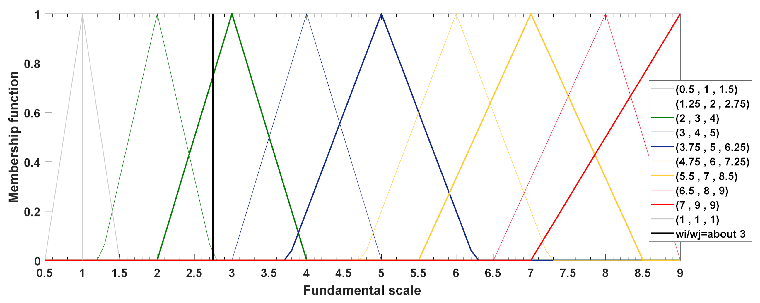
Based on the experts’ knowledge, a fuzzy reciprocal pairwise comparison matrix $\tilde{\mathit{A}}{}_{9\mathit{x}9}$ (Equation (2)) was generated regarding the examined (nine) criteria. Table 1 presents the elements of Saaty’s scale [70] as triangular fuzzy numbers (TFN) (Equation (6)), while the fuzzy judgments of the matrix $\tilde{\mathit{A}}{}_{9\mathit{x}9}$ are presented in Equation (24).

(2)

The optimization problem described in Equation (9) was built and solved by the use of the optimization software LINGO and the weights of criteria (priority vector) were estimated as crisp numbers. Then, the priority vector was normalized based on Equation (10). For space saving reasons, only an example of a pair of inequalities is given regarding the criteria of transmissivity (C₅) and piezometry (C₉). Based on Equation (24) presented below, transmissivity was considered moderate less important in comparison to piezometry; that is $\ln \left(w_5/w_9\right)\approx \left(\frac{1}{4},\frac{1}{3},\frac{1}{2}\right)$. Therefore, it holds:

$$\begin{array}{l}\ln w_5-\ln w_9-\lambda \left(\ln \left((1/3)/(1/4)\right)\right)+{\delta }_{59}\ge \ln (1/4)\\ \ln w_9-\ln w_5-\lambda \left(\ln \left((1/2)/(1/3\right)\right)+n_{59}\ge -\ln (1/2)\end{array}$$

As aforementioned, the parameter M aims to achieve a nonnegative value λ and a small deviation from the fuzzy inequalities constraints which define the fuzzy spread (support set) of each fuzzy judgment. The M-value should ensure a balance between the λ-value and the values of deviation variables [86]. The ideal solution is λ = 1 and ${\displaystyle \sum _{i=1}^{9-1}{\displaystyle \sum _{j=i+1}^9\left({\delta }_{ij}^2+n_{ij}^2\right)}}$ = 0; however, in the real world this is a rare condition [86]. The optimization problem was solved for several M-values. For M = 0.2 it holds: λ = 0.6069 and ${\displaystyle \sum _{i=1}^{9-1}{\displaystyle \sum _{j=i+1}^9\left({\delta }_{ij}^2+n_{ij}^2\right)}}$ = 2.763, for M = 0.5 and hence: λ = 0.317 and ${\displaystyle \sum _{i=1}^{9-1}{\displaystyle \sum _{j=i+1}^9\left({\delta }_{ij}^2+n_{ij}^2\right)}}$ = 1.807.

For or M = 1 it holds: λ = 0.0407 and ${\displaystyle \sum _{i=1}^{9-1}{\displaystyle \sum _{j=i+1}^9\left({\delta }_{ij}^2+n_{ij}^2\right)}}$ = 1.172, while for M > 2 the solutions of deviations converged on ${\displaystyle \sum _{i=1}^{9-1}{\displaystyle \sum _{j=i+1}^9\left({\delta }_{ij}^2+n_{ij}^2\right)}}$ = 1.096 and, the parameter λ = 0.

Therefore, the M-value selected in this study was M = 0.5 since it led to a balanced solution. The solution of the priority vector for M = 0.5 before the normalization was ${\mathit{W}}_{\tilde{A}}^{*}$ = (21.7949, 21.1237, 15.3198, 15.3198, 10.8694, 4.0643, 3.9769, 3.8704, 1.6641), while the normalized weights are presented in Table 2.

Let us verify the above fuzzy constraints regarding the criteria C₅ and C₉. According to the results (for M = 0.5), the deviation variables ${\delta }_{59}$ and $n_{59}$ are zero, therefore:

$$\begin{array}{l}\ln (10.8694)-\ln (21.7949)-0.3174\left(\ln \left((1/3)/(1/4)\right)\right)+0.0\ge \ln (1/4)\hspace{1em}\iff \hspace{1em}-0.78703\ge -1.38629\\ \ln (21.7949)-\ln (10.8694)-0.3174\left(\ln \left((1/2)/(1/3)\right)\right)+0.0\ge -\ln (1/2)\hspace{1em}\iff \hspace{1em}1.35574\ge 0.69315\end{array}$$

which holds.

(3)

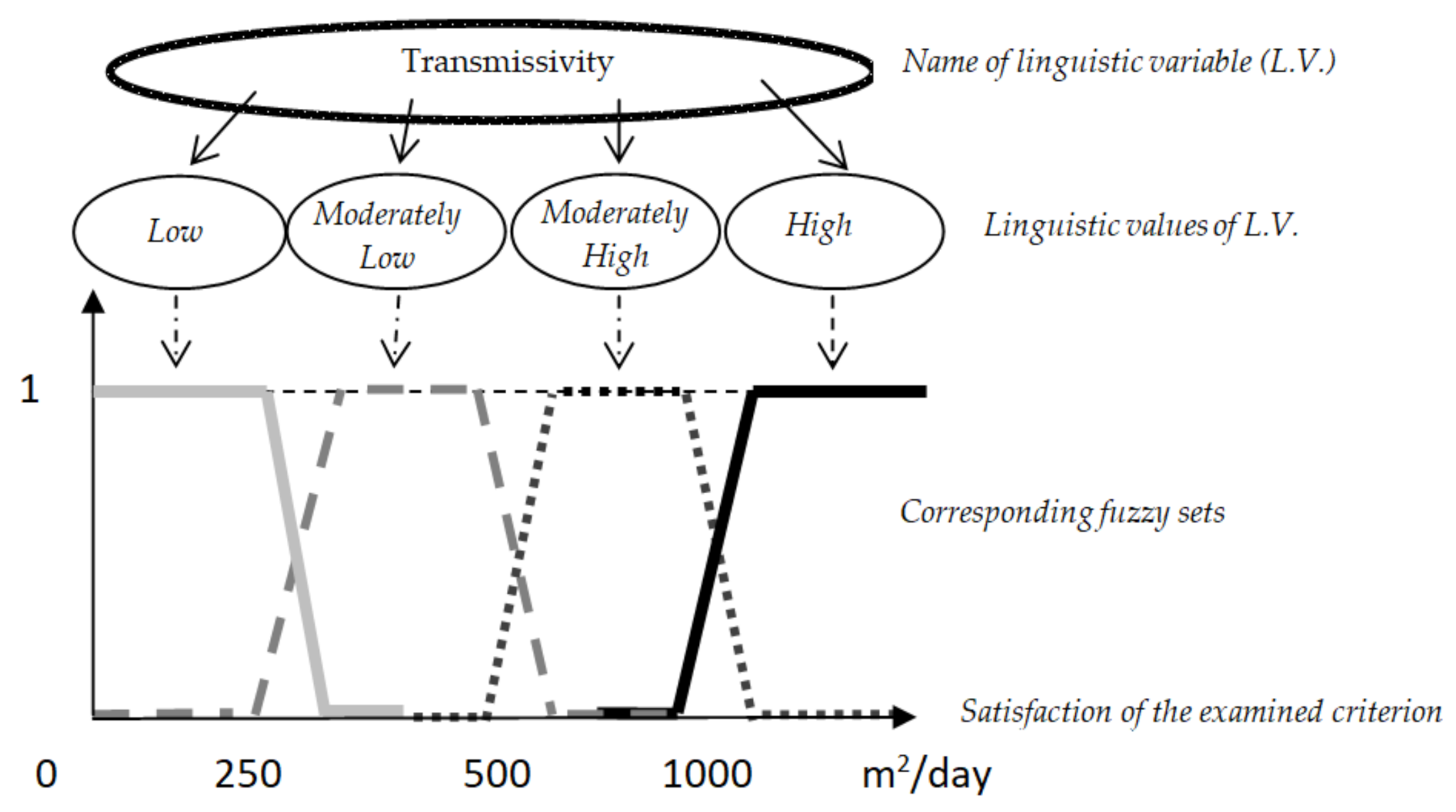
A Mamdani fuzzy inference system, included in the Fuzzy Logic Toolbox of MATLAB, was designed for each criterion. Initially, based on the experts’ judgments, the classes of the examined criteria were fuzzified. The number of classes was determined by using the empirical rule of Sturges [92], which is a common technique in hydrology (Equation (22)):

$$q=1.33\log N$$

(22)

where q is the number of classes and N is the number of data (the numeric value of each alternative regarding the examined criterion, i.e., N = 7).

Then, a system of fuzzy if–then rules (with one input variable, e.g., if slope is low then rating is high) was built (Equation (12)). Both the algebraic product and the min implication were selected to be used in the fuzzy inference process (Equations (19) and (20)). All fuzzy output variables of all rules were combined into a fuzzy conclusion with the max union. Finally, the aggregated fuzzy output was defuzzified based on Equation (21), which is the rating of the each alternative, with respect to each criterion. For the calculation of the rating (R) based on the designed FIS, a simple code was written in MATLAB, which fed the FIS with crisp input data.

(4)

The rating (R) of each alternative was multiplied with the weight of the examined criterion. The final evaluation (final score) of each alternative with respect of all criteria was achieved based on an aggregative model described as follows:

$$A{l}_{u.c.}={\displaystyle \sum _{i=1}^n{w}_i\times R_i}$$

(23)

where $A{l}_{u.c.}$ is the alternative under consideration, $w_i$ is the weight of the criterion i (for n = 9) and $R_i$ is the estimated (by the corresponding FIS) rating of $A{l}_{u.c.}$ regarding the criterion i.

(5)

Based on Equation (23), a rank list of the alternatives (from the most suitable site to the least suitable site for applying MAR) was obtained by using both the algebraic product (Equation (19)) and min implication (Equation (20)) (Table 3). It is noted that although the M-value adopted in this study is equal to 0.5, the results based on M = 1 are also presented in Table 3.

Table 1. Triangular fuzzy numbers (TFN) for the pairwise comparison of the criteria regarding their relative importance.

Relative Importance of Two Criteria	TFN
Equal	(0.5, 1, 1.5)
Moderate	(2, 3, 4)
Strong	(3.75, 5, 6.25)
Very strong	(5.5, 7, 8.5)
Extreme	(7, 9, 9)
Intermediate values	(1.25, 2, 2.75), (3, 4, 5), (4.75, 6, 7.25), (6.5, 8, 9)

Table 1. Triangular fuzzy numbers (TFN) for the pairwise comparison of the criteria regarding their relative importance.

Relative Importance of Two Criteria	TFN
Equal	(0.5, 1, 1.5)
Moderate	(2, 3, 4)
Strong	(3.75, 5, 6.25)
Very strong	(5.5, 7, 8.5)
Extreme	(7, 9, 9)
Intermediate values	(1.25, 2, 2.75), (3, 4, 5), (4.75, 6, 7.25), (6.5, 8, 9)

As shown in the above Table 1, the fuzzy spread increased as the domination between two criteria became stronger. Particularly, a lower fuzzy spread (0.5) corresponds to a judgment of equal importance, “about 1”, while a higher fuzzy spread (2.0) corresponds to a judgment of extreme importance, “about 9”. The authors used this increasing fuzziness on judgments because a wide fuzzy spread in an area of weak domination (i.e., from equal up to moderate importance) may lead to a large overlapping and therefore, two criteria may be considered of “about equal” importance even though they have a weak domination each other (e.g., w_i/w_j = “about 2” or “about 3”). Furthermore, it seems more convenient to accurately adjudicate if two conditions are equal or about equal than to determine the degree of how important a condition is against the other in the case that the importance of the two conditions significantly differs. For instance, a decision maker (DM) might decide more comfortably that ${\tilde{a}}_{1,2}$ = “about 2”, which means that w₁/w₂ might be equal to 3 or equal to 1. On the other hand, in the case that a criterion is much more important than another, making such a judgment that ${\tilde{a}}_{1,7}$ = “about 7”, the real ratio of weights may be equal to 5 or 9, which also denotes significant importance.

It is worth mentioning that several fuzzy spreads were tested. Particularly, constant spreads for the whole scale of Table 1 were used when either the fuzziness was equal to one (e.g., 2, 3, 4) or equal to two (e.g., (1, 3, 5). The tests showed that the weights of the less important criteria increased as the fuzziness increased.

$$\tilde{A}=\begin{array}{c}\begin{array}{ccccccccc}C1\hspace{1em}\hspace{1em}\hspace{1em}& \hspace{1em}C2\hspace{1em}\hspace{1em}\hspace{1em}& \hspace{1em}C3\hspace{1em}\hspace{1em}& \hspace{1em}\hspace{1em}C4\hspace{1em}\hspace{1em}\hspace{1em}& \hspace{1em}C5\hspace{1em}\hspace{1em}\hspace{1em}& \hspace{1em}C6\hspace{1em}\hspace{1em}\hspace{1em}& \hspace{1em}C7& \hspace{1em}\hspace{1em}\hspace{1em}C8& \hspace{1em}\hspace{1em}\hspace{1em}\hspace{1em}C9\end{array}\\ \left[\begin{array}{ccccccccc}1& \left(\frac{1}{4},\frac{1}{3},\frac{1}{2}\right)& \left(\frac{1}{5},\frac{1}{4},\frac{1}{3}\right)& \left(\frac{1}{6.25},\frac{1}{5},\frac{1}{3.75}\right)& \left(\frac{1}{8.5},\frac{1}{7},\frac{1}{5.5}\right)& \left(\frac{1}{9},\frac{1}{8},\frac{1}{6.5}\right)& \left(\frac{1}{9},\frac{1}{8},\frac{1}{6.5}\right)& \left(\frac{1}{9},\frac{1}{9},\frac{1}{7}\right)& \left(\frac{1}{9},\frac{1}{9},\frac{1}{7}\right)\\ \left(2,3,4\right)& 1& \left(\frac{1}{2.75},\frac{1}{2},\frac{1}{1.25}\right)& \left(2,3,4\right)& \left(\frac{1}{5},\frac{1}{4},\frac{1}{3}\right)& \left(\frac{1}{6.25},\frac{1}{5},\frac{1}{3.75}\right)& \left(\frac{1}{6.25},\frac{1}{5},\frac{1}{3.75}\right)& \left(\frac{1}{8.5},\frac{1}{7},\frac{1}{5.5}\right)& \left(\frac{1}{9},\frac{1}{8},\frac{1}{6.5}\right)\\ \left(3,4,5\right)& \left(1.25,2,2.75\right)& 1& \left(\frac{1}{2.75},\frac{1}{2},\frac{1}{1.25}\right)& \left(\frac{1}{5},\frac{1}{4},\frac{1}{3}\right)& \left(\frac{1}{6.25},\frac{1}{5},\frac{1}{3.75}\right)& \left(\frac{1}{6.25},\frac{1}{5},\frac{1}{3.75}\right)& \left(\frac{1}{7.25},\frac{1}{6},\frac{1}{4.75}\right)& \left(\frac{1}{7.25},\frac{1}{6},\frac{1}{4.75}\right)\\ \left(3.75,5,6.25\right)& \left(\frac{1}{4},\frac{1}{3},\frac{1}{2}\right)& \left(1.25,2,2.75\right)& 1& \left(\frac{1}{4},\frac{1}{3},\frac{1}{2}\right)& \left(\frac{1}{5},\frac{1}{4},\frac{1}{3}\right)& \left(\frac{1}{5},\frac{1}{4},\frac{1}{3}\right)& \left(\frac{1}{6.25},\frac{1}{5},\frac{1}{3.75}\right)& \left(\frac{1}{6.25},\frac{1}{5},\frac{1}{3.75}\right)\\ \left(5.5,7,8.5\right)& \left(3,4,5\right)& \left(3,4,5\right)& \left(2,3,4\right)& 1& \left(\frac{1}{2.75},\frac{1}{2},\frac{1}{1.25}\right)& \left(\frac{1}{2.75},\frac{1}{2},\frac{1}{1.25}\right)& \left(\frac{1}{4},\frac{1}{3},\frac{1}{2}\right)& \left(\frac{1}{4},\frac{1}{3},\frac{1}{2}\right)\\ \left(6.5,8,9\right)& \left(3.75,5,6.25\right)& \left(3.75,5,6.25\right)& \left(3,4,5\right)& \left(1.25,2,2.75\right)& 1& \left(\frac{1}{1.5},1,\frac{1}{0.5}\right)& \left(\frac{1}{2.75},\frac{1}{2},\frac{1}{1.25}\right)& \left(\frac{1}{2.75},\frac{1}{2},\frac{1}{1.25}\right)\\ \left(6.5,8,9\right)& \left(3.75,5,6.25\right)& \left(3.75,5,6.25\right)& \left(3,4,5\right)& \left(1.25,2,2.75\right)& \left(0.5,1,1.5\right)& 1& \left(\frac{1}{2.75},\frac{1}{2},\frac{1}{1.25}\right)& \left(\frac{1}{2.75},\frac{1}{2},\frac{1}{1.25}\right)\\ \left(7,9,9\right)& \left(5.5,7,8.5\right)& \left(4.75,6,7.25\right)& \left(3.75,5,6.25\right)& \left(2,3,4\right)& \left(1.25,2,2.75\right)& \left(1.25,2,2.75\right)& 1& \left(\frac{1}{1.5},1,\frac{1}{0.5}\right)\\ \left(7,9,9\right)& \left(6.5,8,9\right)& \left(4.75,6,7.25\right)& \left(3.75,5,6.25\right)& \left(2,3,4\right)& \left(1.25,2,2.75\right)& \left(1.25,2,2.75\right)& \left(0.5,1,1.5\right)& 1\end{array}\right]\end{array}$$

(24)

The following Figure 7 illustrates the scale of the fuzzy judgments of Table 1. For instance, based on Equation (24), the fuzzy pairwise comparison ${\tilde{a}}_{5,9}=\frac{\tilde{1}}{3}\hspace{1em}\iff \hspace{1em}{w}_5/w_9=\frac{\tilde{1}}{3}\hspace{1em}\iff \hspace{1em}{\tilde{a}}_{9,5}=\tilde{3}\hspace{1em}\iff \hspace{1em}{w}_9/w_5=\tilde{3}$ between the criteria C₅ (transmissivity) and C₉ (piezometry) means that piezometry was “about 3” times more significant than transmissivity.

However, an ideal weight ratio (w₅/w₉) between these two criteria exists, which is a crisp number. As aforementioned, the ideal weight ratio of two criteria must be included in the corresponding fuzzy judgment (i.e., the support set of the TFN), or the deviations from the fuzzy thresholds should be small. In the investigation at hand, the black line in Figure 7 is assumed to be this ideal crisp weight ratio w₁/w₅.

The rating of alternatives, the weights before and after normalization, as well as the initial ranges (classes) with their corresponding linguistic variables of the criteria, are presented in Table 2 below. As aforementioned, in the FAHP of Wang and Chin [85], the final weights of criteria are crisp numbers. Based on the experts’ knowledge, the criteria were divided into four crisp classes based on Equation (22). Then, the classes of each criterion were fuzzified and described by linguistic variables (low, moderately low, moderately high, high). These fuzzy classes are illustrated in Figure 8, Figure 9 and Figure 10.

Table 2. Crisp weights of criteria and the rating of alternatives with respect to the classes of criteria. The crisp classes have been fuzzified in FIS.

Criteria	Classes	Linguistic Variable	Rating	Weight	Normalized Weight
C1		High	10	1.6641	0.0169
		Good	8
		Moderate	6
		Deficient	4
		Worse	2
		Unknown	0
C2	0–2	High	10	3.8704	0.0394
	2–5	Moderately high	7.5
	5–10	Moderately low	5
	>10	Low	2.5
C3	<1000	High	10	3.9769	0.0405
	1000–2000	Moderately high	7.5
	2000–3000	Moderately low	5
	>3000	Low	2.5
C4	0–5000	High	10	4.0643	0.0414
	5000–10,000	Moderately high	7.5
	10,000–15,000	Moderately low	5
	>15,000	Low	2.5
C5	>1000	High	10	10.8694	0.1109
	500–1000	Moderately high	7.5
	250–500	Moderately low	5
	0–250	Low	2.5
C6	>0.015	High	10	15.3198	0.1563
	0.005–0.015	Moderately high	7.5
	0.0025–0.005	Moderately low	5
	0–0.0025	Low	2.5
C7	<−1	High	10	15.3198	0.1563
	−1–0	Moderately high	7.5
	0–1	Moderately low	5
	>1	Low	2.5
C8	1	High	10	21.1237	0.2155
	0	Low	0
C9	1	High	10	21.7949	0.2223
	0	Low	0

Table 2. Crisp weights of criteria and the rating of alternatives with respect to the classes of criteria. The crisp classes have been fuzzified in FIS.

Criteria	Classes	Linguistic Variable	Rating	Weight	Normalized Weight
C1		High	10	1.6641	0.0169
		Good	8
		Moderate	6
		Deficient	4
		Worse	2
		Unknown	0
C2	0–2	High	10	3.8704	0.0394
	2–5	Moderately high	7.5
	5–10	Moderately low	5
	>10	Low	2.5
C3	<1000	High	10	3.9769	0.0405
	1000–2000	Moderately high	7.5
	2000–3000	Moderately low	5
	>3000	Low	2.5
C4	0–5000	High	10	4.0643	0.0414
	5000–10,000	Moderately high	7.5
	10,000–15,000	Moderately low	5
	>15,000	Low	2.5
C5	>1000	High	10	10.8694	0.1109
	500–1000	Moderately high	7.5
	250–500	Moderately low	5
	0–250	Low	2.5
C6	>0.015	High	10	15.3198	0.1563
	0.005–0.015	Moderately high	7.5
	0.0025–0.005	Moderately low	5
	0–0.0025	Low	2.5
C7	<−1	High	10	15.3198	0.1563
	−1–0	Moderately high	7.5
	0–1	Moderately low	5
	>1	Low	2.5
C8	1	High	10	21.1237	0.2155
	0	Low	0
C9	1	High	10	21.7949	0.2223
	0	Low	0

As noted, the classes of piezometry, type of aquifer, and ecological status are crisp. Regarding the criteria of piezometry and type of aquifer, two classes were considered and are presented in Appendix B (Figure A2). Therefore, the rating of these alternatives can be either 10 or 0. The criterion of ecological status was divided into six classes based on the relevant national River Basin Management Plans [60]. Since these three criteria divided into crisp classes, the ratings of the alternatives were calculated without the use of FIS.

Table 3 and Figure 11 present the final rating of the alternatives resulting from using either the min implication or the fuzzy implication of the algebraic product, for M = 1 and M = 2. As shown in Table 3, the ranking order of the alternatives (Al₅ > Al₂ > Al₁ > Al₄ > Al₇ > Al₆ > Al₃) was identical in almost all cases. A slight variation between the latter options took place when the min implication was used, and the M-value was equal to M = 1 (Al₅ > Al₂ > Al₁ > Al₄ > Al₇ > Al₃ > Al₆).

Table 3. Final evaluation of the alternatives based on Mamdani product and min implication.

Ranking Order/ Implication	Alg. Prod. (M = 0.5)	Min (M = 0.5)	Alg. Prod. (M = 1)	Min (M = 1)
Al5	8.0317	8.0320	7.9846	7.9792
Al2	7.9859	7.9932	7.9355	7.9370
Al1	7.7936	7.7877	7.7329	7.7191
Al4	7.3382	7.3611	7.2765	7.2939
Al7	6.5145	6.5179	6.4232	6.4228
Al6	4.6199	4.6045	4.5888	4.5712
Al3	4.5822	4.5829	4.5508	4.7090

Table 3. Final evaluation of the alternatives based on Mamdani product and min implication.

Ranking Order/ Implication	Alg. Prod. (M = 0.5)	Min (M = 0.5)	Alg. Prod. (M = 1)	Min (M = 1)
Al5	8.0317	8.0320	7.9846	7.9792
Al2	7.9859	7.9932	7.9355	7.9370
Al1	7.7936	7.7877	7.7329	7.7191
Al4	7.3382	7.3611	7.2765	7.2939
Al7	6.5145	6.5179	6.4232	6.4228
Al6	4.6199	4.6045	4.5888	4.5712
Al3	4.5822	4.5829	4.5508	4.7090

5. Discussion

According to the results (Table 3 and Figure 11), the more favorable sites (Al₅ > Al₂ > Al₁) for applying floodwater spreading were located, in general, in the northwest of the study area. Particularly, Al₅ was the most preferable alternative in all cases. In contrast, the final ratings of the alternatives located in the southeast part of the area under investigation were low (less favorable alternatives). This may be partly explained by the composition of geological formations which range from fine to silty clay in the SE–E direction towards Vistonida Lagoon [53,55]. However, this is not an absolute condition due to the significant variability of alluvial composition in the study area [58] on the one hand, and the contribution of the other criteria in the analysis on the other. For instance, the alternatives A₁ and Al₆ were less preferable than Al₂. Certainly, in the case of evaluating just a few alternatives, the best alternative might be identified on the basis of traditional hydrogeological analysis even though the criteria weights would not be taken into account. However, the more alternatives and criteria, the more complexity for the selection of the most preferable recharge site by an expert. Moreover, it is desirable that the MAR application is as effective as possible given its not negligible cost [93], and thus the solution of the selection problem should really be the best. As pointed out, the proposed methodology can be applied on both a large and small number of alternatives/criteria and this is a merit of the proposed methodology.

The local conditions of the case study (e.g., sparsely populated flat area) favor the application of flood spreading methods through infiltration basins, inasmuch as the excess winter water of the Kosynthos River might be used. Thus, the criteria were selected according to this type of MAR focusing on the hydrogeological local characteristics. Other criteria, such as socioeconomic and technical criteria, were not taken into account, as they are more in line with the design and implementation of MAR. It is worth mentioning that all alternatives were located south of the Kosynthos River. This is due to the fact that the Kosynthos River is the north hydraulic boundary of the aquifer system in the Xanthi plain [56,57,58].

The criteria weights were obtained through the FAHP–LFFP-based nonlinear method. Thus, in contrast to the conventional AHP, fuzziness was used to incorporate the uncertainty from the subjectivity of the initial experts’ judgments. Using the FAHP–LFFP-based nonlinear method, a potential zero weight value was avoided and the non negativity of the λ-value was ensured, generating a unique optimal crisp priority vector. Besides, by using the FAHP–LFFP-based nonlinear method, the analysis could be performed either on the upper triangular elements of the fuzzy pairwise comparison matrix or on the lower ones. However, fuzzy weights can be obtained with the use of other methods (e.g., [94]).

An interesting point for discussion is the fuzziness of the initial judgments. In this study, an increasing fuzzy spread (width) was adopted regarding the scale of relative importance between two criteria. A reason for this was to avoid a large overlapping in the weak domination area that could lead to assigning almost equal importance to criteria even though there was a weak or moderately weak domination between the two criteria. Moreover, it seems more comfortable for a DM to assess that two conditions are equal or about equal than to assign the degree of their relative importance when their importance significantly differs. It is worth mentioning that after several tests on fuzzy spreads, which for space saving reasons are not presented, it was found that by increasing the fuzziness, the weights of the less important criteria increased (i.e., distance from road network, distance from hydrographic network, slope, and ecological status).

Regarding the parameter M used in the FAHP–LFFP method, it aims to ensure the nonnegativity of parameter λ and to allow little deviation from fuzzy inequalities constraints, and hence an optimal solution that simultaneously satisfies all the fuzzy judgments can be achieved. An interesting point is that for M > 2, the solutions of deviations converged on a unit which had the lowest value in comparison with the solutions of deviation for M < 2. However, the λ-value was zero, which means that the inequalities of Equation (8) did not simultaneously hold, and thus these values were not used. The M-value selected was M = 0.5 because it produced a more balanced solution between the λ-value and the total deviations than those that were produced when M = 1 and M = 0.2 were used. In the calculation of the λ-value, the fuzzy min intersection was used because using the other widely used t-norm (algebraic product) resulted in a lower satisfaction degree of the fuzzy pairwise comparisons.

The ratings of the alternatives with respect to each criterion were based on using fuzzy inferences systems based on the Mamdani approach. The use of such systems was preferred in this study in order for the ranges (classes) of criteria to be fuzzified. The ranges of criteria were modulated on the basis of the available information (e.g., min–max values of each criterion regarding the case study) and of the experts’ knowledge. Therefore, it seemed more reasonable to use fuzzy thresholds of the ranges than crisp ones for taking into account the uncertainty derived from the lack of information and imprecise knowledge.

Another reason for using FIS is that, there are not precise and well-known objective functions for each criterion, as in the usual multi-objective problems.

On the other hand, the selection problem examined in this study could be solved based on the exclusive use of FIS; however, this choice was not preferred because it would lead to a complex system of fuzzy if-then rules.

In this study, each FIS is based on a simple system of fuzzy if-then rules, where only an input variable, has been used (Equation (12)). Therefore, neither t-conorms nor t-norms were used in the antecedent if-part. As the fuzzy implication is concerned, both the two widely used fuzzy implications were used. That is, the Mamdani implication, in which the t-norm of algebraic product is used, and the min implication, in which the t-norm of min intersection is used. In general, in case of no distinction between cause and effect, the min fuzzy implication is recommended. However, several other fuzzy implications can be used [95], the appropriate selection of which is an open issue [90]. For the composition of the fuzzy rules, the widely used t-conorm of max union was preferred. However, other t-conorms can also be tested. The fuzzy output of each FIS method is defuzzified by selecting the centroid method, which is considered a balanced solution given that it counts the gravity center.

The synthesis of criteria with respect of each alternative was achieved based on a simple additive model, in which the rating (the defuzzified output of the FIS) of each alternative is multiplied with the normalized weight with respect of each criterion. The total sum is the final evaluation (final score) of each alternative. The alternative with the highest score is the solution to the decision-making problem. Other (fuzzy) multi attributes decision-making (MADM) methods might be used for the synthesis of criteria and the final ranking of alternatives using the weights derived by the FAHP–LFFP-based nonlinear method (e.g., fuzzy TOPSIS, fuzzy ELECTRE, fuzzy pattern recognition). However, the use of such methods would have increased the complexity of the solution process on one hand and more information would have been required on the other.

The FAHP–LFFP method and the FIS were applied to the examined problem for the first time. According to Table 3, the solution (ranking order of the alternatives) did not changed regardless of which M-value or fuzzy inference engine was used, except in the case of min implication, in which the less preferable alternatives exchanged order. Thus, based on the knowledge of previous studies [53,55,56,57,58,60] regarding the hydrogeological conditions of the case study, and by taking into account the stability of the solution, the results of the proposed methodology are considered reliable. It would be of great interest if these results were compared with those of other (hybrid) multi-criteria methods that could be applied in the composition of criteria (e.g., fuzzy ELECTRE, fuzzy pattern recognition).

6. Conclusions

This research applied a hybrid fuzzy multi-criteria methodology to select preferable site for applying MAR systems in the context of increasing the local groundwater availability for later water use in case of drought occurrence. Fuzzy set theory and fuzzy logic were used both in the determination of criteria weights and in the evaluation of alternatives, thus incorporating the uncertainties derived from the subjectivity and the lack of information.

The proposed methodology was applied in a flat agricultural area in the southeast of Xanthi city, northern Greece, where a significant number of irrigation wells draw from the shallow aquifer system. The local conditions favor the implementation of flood spreading through infiltration basins utilizing excess winter water of the Kosynthos River.

The results show that:

(1)

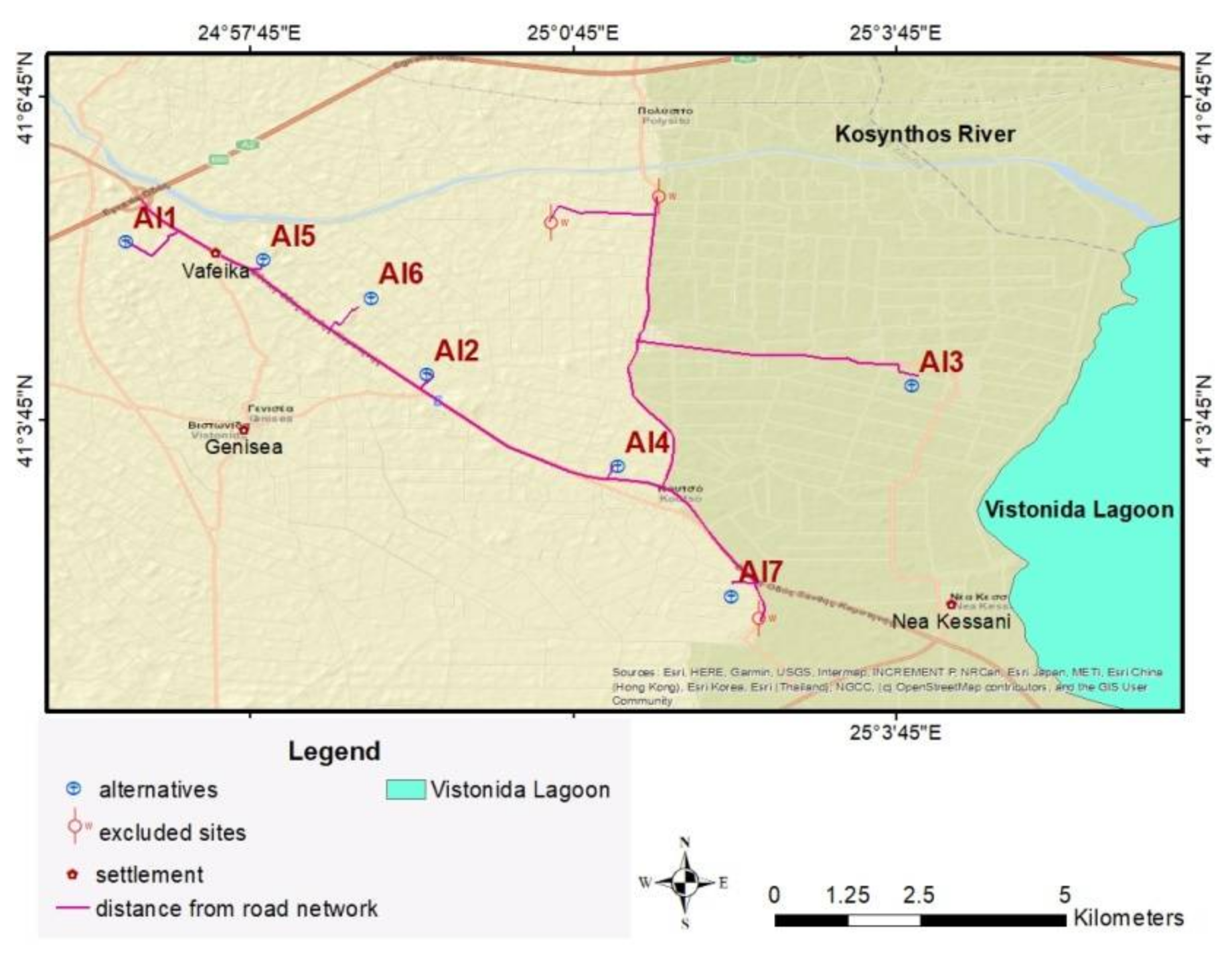
The more preferable sites are located in the northwestern part of the study area near the Kosynthos River, while the most preferable is the Al₅ alternative. This mainly holds due to the hydrological conditions of the northwestern part, which are more favorable than the southeastern ones for groundwater recharge. However, this is not an absolute condition due to the intense diversity of geological formations. In addition, the contribution of the analysis of the other criteria also affected the final rank list.

(2)

The proposed methodology can be used for distinguishing discrete preferable points (alternatives) for MAR application without limitation in number of the examined alternatives. In addition, the selected criteria can be added or subtracted depending on specific local conditions. In case of application of another type of MAR the selected criteria should be adjusted as well. Certainly, in the case of a small number (<10) of alternatives to study, a classical hydrogeological analysis may lead to the selection of the most preferable alternative. However, in that case, the criteria weights would not be taken into account and thus, there would be the possibility of not obtaining an efficient and comprehensive solution. On the other hand, in the case of a large number of examined alternatives and criteria, where the complexity increased, the proposed methodology might be also a useful tool for ranking discrete alternatives. Other than that, it could be used as an alternative way to identify suitable recharge sites in case of low data availability.

(3)

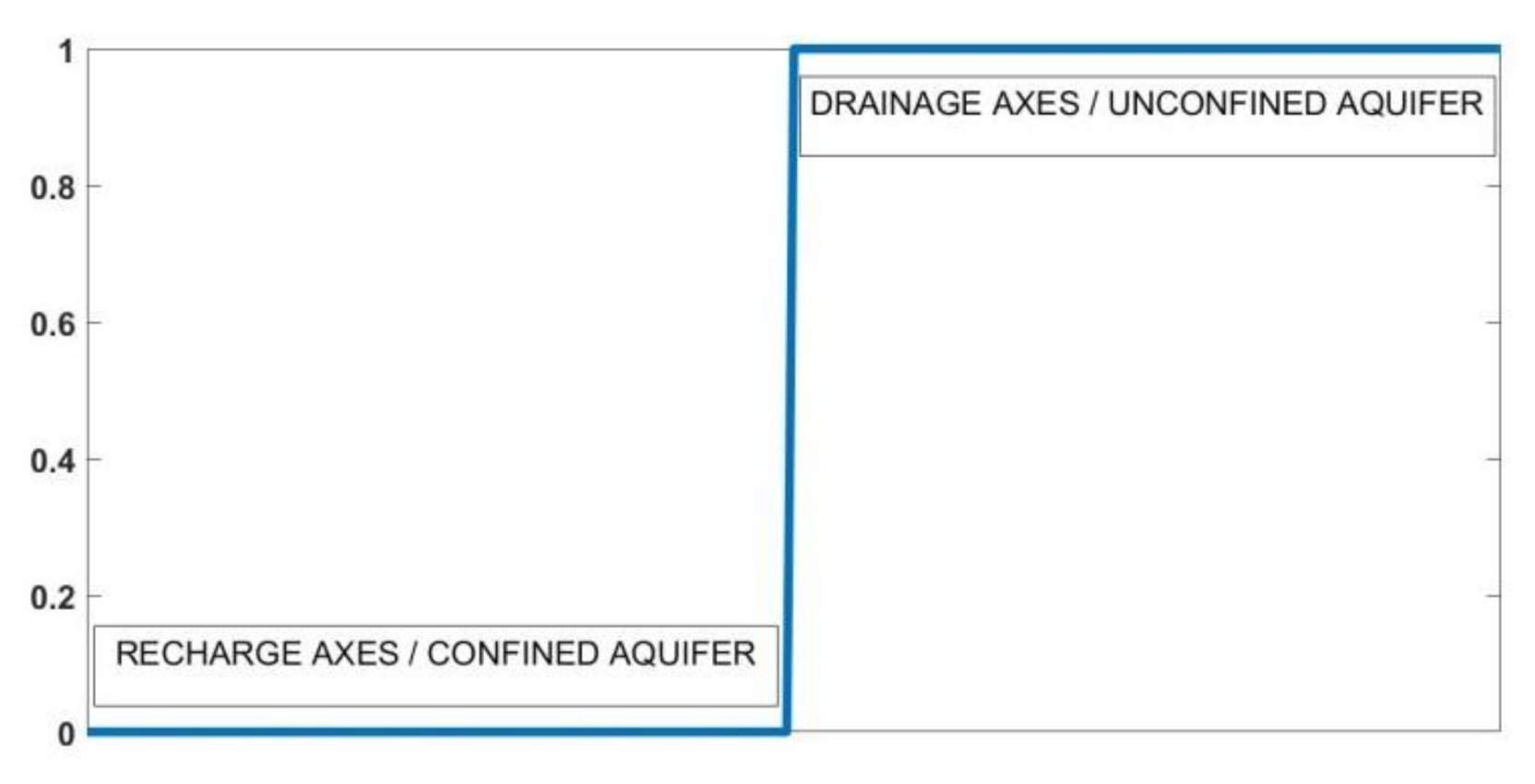
The applicability of the methodology requires lithological profile and hydraulic characteristics of both vadose and saturated zones, while it can be applied only in unconfined aquifers and where there is an underlying drainage axis. Furthermore, the application of this type of MAR requires the presence of a river whose excess waters can be utilized. Thus, after a preparatory screening, seven alternatives satisfied all the assumptions and criteria were finally evaluated.

(4)

In general, the use of fuzzy logic in AHP can incorporate the uncertainty from the subjectivity of the initial experts’ judgments, while the fuzzy version of AHP implemented in this paper (FAHP–LFFP-based nonlinear method) can ensure a unique and optimal solution.

(5)

Fuzzy inference systems (FIS) based on Mamdani’s approach are used in order to determine the rating of each alternative, since the objective function (or value function) regarding each examined criterion is unknown. In addition, with use of FIS, the classes of criteria are fuzzified, and this fact is more reasonable to describe the real conditions.

References

- Vörösmarty, C.J.; Green, P.; Salisbury, J.; Lammers, R.B. Global Water Resources: Vulnerability from Climate Change and Population Growth. Science 2000, 289, 284–288. [Google Scholar] [CrossRef]
- Tebaldi, C.; Hayhoe, K.; Arblaster, J.M.; Meehl, G.A. Going to the extremes. Clim. Chang. 2006, 79, 185–211. [Google Scholar] [CrossRef]
- Taylor, R.G.; Scanlon, B.; Döll, P.; Rodell, M.; Van Beek, R.; Wada, Y.; Longuevergne, L.; Leblanc, M.; Famiglietti, J.S.; Edmunds, M.; et al. Ground water and climate change. Nat. Clim. Chang. 2013, 3, 322–329. [Google Scholar] [CrossRef]
- Zwiers, F.W.; Alexander, L.V.; Hegerl, G.C.; Knutson, T.R.; Kossin, J.P.; Naveau, P.; Nicholls, N.; Schär, C.; Seneviratne, S.I.; Zhang, X. Climate extremes: Challenges in estimating and understanding recent changes in the frequency and intensity of extreme climate and weather events. In Climate Science for Serving Society; Asrar, G.R., Hurrell, J.W., Eds.; Springer: Dordrecht, The Netherlands, 2013; pp. 339–389. ISBN 978-94-007-6691-4. [Google Scholar]
- Wuebbles, D.; Meehl, G.; Hayhoe, K.; Karl, T.R.; Kunkel, K.; Santer, B.; Wehner, M.; Colle, B.; Fischer, E.M.; Fu, R.; et al. CMIP5Climate Model Analyses: Climate Extremes in the United States. Bull. Am. Meteor. Soc. 2013, 95, 571–583. [Google Scholar] [CrossRef]
- Bouwer, H. Artificial recharge of groundwater:hydrogeology and engineering. Hydrogeol. J. 2000, 10, 121–142. [Google Scholar]
- Maliva, R.G.; Guo, W.; Missimer, T.M. Aquifer storage and recovery: Recent hydrogeological advances and system performance. Water Environ. Res. 2006, 78, 2428–2435. [Google Scholar] [CrossRef]
- Jager, H.I.; Smith, B.T. Sustainable Reservoir Operation: Can We Generate Hydropower and Preserve Ecosystem Values? River Res. Appl. 2008, 24, 340–352. [Google Scholar] [CrossRef]
- Minsley, B.J.; Ajo-Franklin, J.; Mukhopadhyay, A.; Morgan, F.D. Hydrogeophysical Methods for Analyzing Aquifer Storage and Recovery Systems. Groundwater 2011, 49, 250–269. [Google Scholar] [CrossRef]
- Giordano, M. Global Groundwater? Issues and Solutions. Annu. Rev. Environ. Resour. 2009, 34, 153–178. [Google Scholar] [CrossRef]
- Kundzewicz, Z.W.; Doll, P. Will groundwater ease freshwater stress under climate change? Hydrol. Sci. J. 2009, 54, 665–675. [Google Scholar] [CrossRef]
- Scanlon, B.R.; Reedy, R.C.; Faunt, C.C.; Pool, D.; Uhlman, K. Enhancing drought resilience with conjunctive use and managed aquifer recharge in California and Arizona. Environ. Res. Lett. 2016, 11, 035013. [Google Scholar]
- de Graaf, I.E.M.; Gleeson, T.; Rens van Beek, L.P.H.; Sutanudjaja, E.H.; Bierkens, M.F.P. Environmental Flow Limits to Global Groundwater Pumping. Nature 2019, 574, 90–94. [Google Scholar] [CrossRef]
- Dillon, P. Future management of aquifer recharge. Hydrogeol. J. 2005, 13, 313–316. [Google Scholar] [CrossRef]
- Niswonger, R.G.; Morway, E.D.; Triana, E.; Huntington, J.L. Managed aquifer recharge through off-season irrigation in agricultural regions. Water Resour. Res. 2017, 53, 6970–6992. [Google Scholar] [CrossRef]
- California Department of Water Resources. Using Flood Water for Managed Aquifer Recharge to Support Sustainable Water Resources. White Paper. 26 June 2018, p. 54. Available online: https://ui.adsabs.harvard.edu/abs/2018AGUFM.H51X1679M/abstract (accessed on 30 December 2021).
- Dillon, P.; Stuyfzand, P.; Grischek, T.; Lluria, M.; Pyne, R.D.G.; Jain, R.C.; Bear, J.; Schwarz, J.; Wang, W.; Fernandez, E.; et al. Sixty years of global progress in managed aquifer recharge. Hydrogeol. J. 2019, 27, 1–30. [Google Scholar] [CrossRef]
- Wendt, D.E.; Van Loon, A.F.; Scanlon, B.R.; Hannah, D.M. Managed Aquifer Recharge as a Drought Mitigation Strategy in Heavily-Stressed Aquifers. Environ. Res. Lett. 2021, 16, 014046. [Google Scholar] [CrossRef]
- Zhao, M.; Boll, J.; Adam, J.C.; King, A.B. Can Managed Aquifer Recharge Overcome Multiple Droughts? Water 2021, 13, 2278. [Google Scholar] [CrossRef]
- Gale, I.N.; Dillon, P. Strategies for Managed Aquifer Recharge (MAR) in Semi-Arid Areas; United Nations Educational, Scientific and Cultural Organisation (UNESCO): Paris, France, 2005; p. 30. [Google Scholar]
- Ringleb, J.; Sallwey, J.; Stefan, C. Assessment of Managed Aquifer Recharge through Modeling—A Review. Water 2016, 8, 579. [Google Scholar] [CrossRef]
- Foster, S.; van Steenbergen, F. Conjunctive groundwater use: A ‘lost opportunity’ for water management in the developingworld? Hydrogeol. J. 2011, 19, 959–962. [Google Scholar] [CrossRef]
- Maliva, R.G. Antropogenic Aquifer Recharge; WSP Methods in Water Resources Evaluation Series No. 5; Springer: Cham, Switzerland, 2020; p. 861. [Google Scholar] [CrossRef]
- Dillon, P.; Escalante, E.F.; Tuinhof, A. Management of Aquifer Recharge and Discharge Processes and Aquifer Storage Equilibrium; Groundwater Governance Thematic Paper 4; GEF-FAO: Rome, Italy, 2012. [Google Scholar]
- Pakparvar, M.; Walraevens, K.; Cheraghi, S.A.M.; Cornelis, W.; Gabriels, D.; Kowsar, S.A. Assessment of groundwater recharge influenced by floodwater spreading: An intergrated approach with limited accessible data. Hydrol. Sci. J. 2017, 62, 147–164. [Google Scholar] [CrossRef]
- Hashemi, H.; Berndtsson, R.; Persson, M. Artificial recharge by floodwater spreading estimated by water balancesand groundwater modeling in arid Iran. Hydrol. Sci. J. 2015, 60, 336–350. [Google Scholar] [CrossRef]
- Saraf, A.K.; Choudhury, P.R. Integrated remote sensing and GIS for ground waterexploration and identification of artificial recharge sites. Int. J. Remote Sens. 1998, 19, 1825–1841. [Google Scholar] [CrossRef]
- Al Saud, M. Mapping potential areas for groundwater storage in Wadi Aurnah Basin, western Arabian Peninsula, using remote sensing and geographic information system techniques. Hydrogeol. J. 2010, 18, 1481–1495. [Google Scholar] [CrossRef]
- Senanayake, I.P.; Dissanayake, D.M.D.O.K.; Mayadunna, B.B.; Weerasekera, W.L. An approach to delineate groundwater recharge potential sites in Ambalantota, Sri Lanka using GIS techniques. Geosci. Front. 2016, 7, 115–124. [Google Scholar] [CrossRef]
- Chenini, I.; Ben Mammou, A.; El May, M. Groundwater Recharge Zone Mapping Using GIS-Based Multi-criteria Analysis: A Case Study in Central Tunisia (Maknassy Basin). Water Resour. Manag. 2010, 24, 921–939. [Google Scholar] [CrossRef]
- Chowdhury, A.; Jha, M.K.; Chowdary, V.M. Delineation of groundwater recharge zones and identification of artificial recharge sites in West Medinipur district, West Bengal, using RS, GIS and MCDM techniques. Environ. Earth Sci. 2010, 59, 1209–1222. [Google Scholar] [CrossRef]
- Nasiri, H.; DarvishiBoloorani, A.; FarajiSabokbar, H.A.; Jafari, H.R.; Hamzeh, M.; Rafi, Y. Determining the most suitable areas for artificial groundwater recharge via an integrated PROMETHEE II-AHP method in GIS environment (case study: Garabaygan Basin, Iran). Environ. Monit. Assess. 2013, 185, 707–718. [Google Scholar] [CrossRef]
- Valverde, J.P.B.; Blank, C.; Roidt, M.; Schneider, L.; Stefan, C. Application of a GIS Multi-Criteria Decision Analysis for the Identification of Intrinsic Suitable Sites in Costa Rica for the Application of Managed Aquifer Recharge (MAR) through Spreading Methods. Water 2016, 8, 391. [Google Scholar] [CrossRef]
- Selvarani, A.G.; Maheswaran, G.; Elangovan, K. Identification of artificial recharge sites for Noyyal River Basin using GIS and remote sensing. J. Indian Soc. Remote Sens. 2017, 45, 67–77. [Google Scholar] [CrossRef]
- Kazakis, N. Delineation of Suitable Zones for the Application of Managed Aquifer Recharge (MAR) in Coastal Aquifers Using Quantitative Parameters and the Analytical Hierarchy Process. Water 2018, 10, 804. [Google Scholar] [CrossRef]
- Zadeh, L.A. Fuzzy sets. Inf. Control 1965, 8, 338–353. [Google Scholar]
- Zimmermann, H.-J. Advanced Review. Fuzzy set theory. WIREs Comput. Stat. 2010, 2, 317–332. [Google Scholar] [CrossRef]
- Garg, H. A Hybrid GA-GSA Algorithm for Optimizing the Performance of an Industrial System by Utilizing Uncertain Data. In Handbook of Research on Artificial Intelligence Techniques and Algorithms; Pandian, V., Ed.; IGI Global: Hershey, PE, USA, 2015; pp. 620–654. [Google Scholar] [CrossRef]
- Bogardi, I.; Duckstein, L.; Bardossy, A. Regional management of an aquifer under fuzzy environmental objectives. Water Resour. Res. 1983, 19, 1394–1402. [Google Scholar] [CrossRef]
- Kambalimath, S.; Deka, P.C. A basic review of fuzzy logic applications in hydrology and water resources. Appl. Water Sci. 2020, 10, 191. [Google Scholar] [CrossRef]
- Kazakis, N.; Spiliotis, M.; Voudouris, K.; Pliakas, F.K.; Papadopoulos, B. A fuzzy multicriteria categorization of the GALDIT method to assess seawater intrusion vulnerability of coastal aquifers. Sci. Total Environ. 2018, 621, 524–534. [Google Scholar] [CrossRef]
- Kourgialas, N.N.; Anyfanti, I.; Karatzas, G.P.; Dokou, Z. An integrated method for assessing drought prone areas-Water efficiency practices for a climate resilient Mediterranean agriculture. Sci. Total Environ. 2018, 625, 1290–1300. [Google Scholar] [CrossRef]
- Spiliotis, M.; Iglesias, A.; Garrote, L. A multicriteria fuzzy pattern recognition approach for assessing the vulnerability to drought: Mediterranean region. Evol. Syst. 2021, 12, 109–122. [Google Scholar] [CrossRef]
- Chan, F.T.S.; Kumar, N. Global supplier development considering risk factors using fuzzy extended AHP-based approach. Omega 2007, 35, 417–431. [Google Scholar] [CrossRef]
- Chan, F.T.S.; Kumar, N.; Tiwari, M.K.; Lau, H.C.W.; Choy, K.L. Global supplier selection: A fuzzy-AHP approach. Int. J. Prod. Res. 2008, 46, 3825–3857. [Google Scholar] [CrossRef]
- Saravi, M.M.; Malekian, A.; Nouri, B. Identification of Suitable Sites for Groundwater Recharge. In Proceedings of the 2nd International Conference on Water Resources & Arid Environment, Riyadh, Saudi Arabia, 26–29 November 2006; pp. 1–5. [Google Scholar]
- Ghayoumian, J.; MohseniSaravi, M.; Feiznia, S.; Nouri, B.; Malekian, A. Application of GIS techniques to determine areas most suitable for artificial groundwater recharge in a coastal aquifer in southern Iran. J. Asian Earth Sci. 2007, 30, 364–374. [Google Scholar] [CrossRef]
- Riad, P.H.; Billib, M.H.; Hasan, A.A.; Omar, M.A. Overlay Weighted Model and Fuzzy Logic to Determine the Best Locations for Artificial Recharge of Groundwater in a Semi-Arid Area in Egypt. Nile Basin Water Sci. Eng. J. 2011, 4, 24–35. [Google Scholar]
- Malekmohammadi, B.; Mehrian, M.R.; Jafari, H.R. Site selection for managed aquifer recharge using fuzzy rules: Integrating geographical information system (GIS) tools and multi-criteria decision making. Hydrogeol. J. 2012, 20, 1393–1405. [Google Scholar] [CrossRef]
- Dashtpagerdi, M.M.; Vagharfard, H.; Honarbakhsh, A.; Khoorani, A. GIS Based Fuzzy Logic Approach for Identification of Groundwater Artificial Recharge Site. Open J. Geol. 2013, 3, 379–383. [Google Scholar] [CrossRef][Green Version]
- Selvarani, A.G.; Maheswaran, G.; Elangovan, K. Identification of Artificial Recharge Sites For Noyyal Watershed Using GIS And Fuzzy Logic. Int. J. Appl. Eng. Res. 2015, 10, 11189–11208. [Google Scholar]
- Ghasemi, A.; Saghafian, B.; Golian, S. Optimal location of artificial recharge of treated wastewater using fuzzy logic approach. J. Water Supply Res. Technol. 2017, 66, 141–156. [Google Scholar] [CrossRef]
- Pliakas, F.; Kallioras, A.; Damianidis, P.; Kostakakis, P. Evaluation of precipitation effects on groundwater levels in a Mediterranean alluvial plain based on hydrogeological conceptualization. Environ. Earth Sci. 2015, 74, 3573–3588. [Google Scholar] [CrossRef]
- Dimadis, E.; Zachos, S. Geological Map of Rhodope Massif; Institute of Geology and Mineral Exploration (IGME), Regional Subdivision of Eastern Macedonia—Thrace: Xanthi, Greece, 1986. [Google Scholar]
- Sakkas, I.; Diamantis, I.; Pliakas, F. Groundwater Artificial Recharge Study of Xanthi-Rhodope Aquifers (in Thrace, Greece); Greek Ministry of Agriculture Research Project, Final Report; Sections of Geotechnical Engineering and Hydraulics of the Civil Engineering Department of Democritus University of Thrace: Xanthi, Greece, 1998. (In Greek)
- Pliakas, F.; Diamantis, I.; Petalas, C. Results from a Groundwater Artificial Recharge Application in Polysitos Aquifer at Xanthi Plain Region (Greece) by Reactivating Old Stream Beds. In Proceedings of the 5th Greek National Hydrogeological Conference, Nicosia, Cyprus, 12−14 November 1999; pp. 97–113. (In Greek). [Google Scholar]
- Pliakas, F.; Petalas, C.; Diamantis, I.; Kallioras, A. Modeling of groundwater artificial recharge by reactivating an on old streambed. Water Resour. Manag. 2005, 19, 279–294. [Google Scholar]
- Pisinaras, V. Aνάπτυξη ΕνόςΠλαισίου OλοκληρωμένηςΔιαχείρισης Πολύπλοκων Συστημάτων ΥπόγειωνΥδατικών πόρων [Development of a Methodology Framework for Integrated Management of Complex Groundwater Systems]. Ph.D. Thesis, Democritus University of Thrace, Xanthi, Greece, June 2008. (In Greek). [Google Scholar]
- Papadopoulos, C.; Spiliotis, M.; Gkiougkis, I.; Pliakas, F.; Papadopoulos, B. Fuzzy linear regression analysis for groundwater response to meteorological drought in the aquifer system of Xanthi plain, NE Greece. J. Hydroinform. 2021, 23, 1112–1129. [Google Scholar] [CrossRef]
- Diamantis, I.; Pliakas, F.; Petalas, C. The contribution of artificial recharge as a remedy procedure regarding the impacts of various interventions on the natural environment of plain regions. The case study in Thrace, Greece. In Proceedings of the International Symposium on Engineering Geology and the Environment, Organized by the Greek National Group of the International Association for Engineering Geology and the Environment (IAEG), Athens, Greece, 23–27 June 1997; pp. 2663–2667. [Google Scholar]
- Special Secretariat for Water. River Basin Management Plans of Thrace Water District (GR12); Ministry of Environmental and Energy: Athens, Greece, 2017.
- Krishnamurthy, J.; Kkumar, N.V.; Jayaraman, V.; Manivel, M. An approach to demarcate ground water potential zones through remote sensing and geographic information system. Int. J. Remote Sens. 1996, 17, 1867–1884. [Google Scholar]
- Farhadian, M.; Bozorg-Haddad, O.; Pazoki, M.; Loaiciga, H.A. Locating and Prioritizing Suitable Places forthe Implementation of Artificial Groundwater Recharge Plans. J. Irrig. Drain. Eng. 2017, 143, 04017018. [Google Scholar]
- Ghayoumian, J.; Ghermezcheshmeh, B.; Feiznia, S.; Noroozi, A.A. Integrating GIS and DSS for identification of suitable areas for artificial recharge, case study Meimeh Basin, Isfahan. Iran. Environ. Geol. 2005, 47, 493–500. [Google Scholar]
- Jasrotia, A.S.; Kumar, R.; Saraf, A.K. Delineation of groundwater recharge sites using integrated remote sensing and GIS in Jammu district, India. Int. J. Remote Sens. 2007, 28, 5019–5036. [Google Scholar]
- Klir, G.J.; Yuan, B. Fuzzy Sets and Fuzzy Logic. Theory and Applications; Prentice Hall: Hoboken, NJ, USA, 1995. [Google Scholar]
- Ross, T.J. Fuzzy Logic with Engineering Applications, 3rd ed.; John Wiley & Sons: West Sussex, UK, 2010; p. 585. [Google Scholar]
- Zimmerman, H.-J. Fuzzy Set Theory and Its Applications, 4th ed.; Springer Science & Business Media: New York, NY, USA, 2001; p. 514. [Google Scholar]
- Wang, L.-X. A Course in Fuzzy Systems and Control; Prentice Hall: Hoboken, NJ, USA, 1997; p. 424. [Google Scholar]
- Saaty, T.L. The Analytic Hierarchy Process; McGraw-Hill: New York, NY, USA, 1980. [Google Scholar]
- Pöyhönen, M.A.; Hämäläinen, R.P.; Salo, A.A. An Experiment on the Numerical Modeling of Verbal Ratio Statements. J. Multi-Criteria Decis. Anal. 1997, 6, 1–10. [Google Scholar]
- Ho, W.; Ma, X. The state-of-the-art integrations and applications of the analytic hierarchy process. Eur. J. Oper. Res. 2018, 267, 399–414. [Google Scholar] [CrossRef]
- Chang, D.-Y. Applications of the extent analysis method on fuzzy AHP. Theory and Methodology. Eur. J. Oper. Res. 1996, 95, 649–655. [Google Scholar]
- Kwong, C.K.; Bai, H. Determining the importance weights for the customer requirements in QFD using a fuzzy AHP with anextent analysis approach. IIE Trans. 2003, 35, 619–626. [Google Scholar]
- Kahraman, C.; Ruan, D.; Dogan, I. Fuzzy group decision making for facility location selection. Inf. Sci. 2003, 157, 135–153. [Google Scholar]
- Kahraman, C.; Ertay, T.; Buyukozkan, G. A fuzzy optimization model for QFD planning process using analytic network approach. Eur. J. Oper. Res. 2006, 171, 390–411. [Google Scholar]
- Srdjevic, B.; Medeiros, Y.D.P. Fuzzy AHP Assessment of Water Management Plan. Water Resour. Manag. 2008, 22, 877–894. [Google Scholar] [CrossRef]
- Wang, Y.-M.; Luo, Y.; Hua, Z. On the extent analysis method for fuzzy AHP and its applications. Eur. J. Oper. Res. 2008, 186, 735–747. [Google Scholar] [CrossRef]
- Mikhailov, L. Deriving priorities from fuzzy pairwise comparison judgements. Fuzzy Sets Syst. 2003, 134, 365–385. [Google Scholar] [CrossRef]
- Mikhailov, L. A fuzzy programming method for deriving priorities in the analytic hierarchy process. J. Oper. Res. Soc. 2000, 51, 341–349. [Google Scholar] [CrossRef]
- Li, L.; Lai, K.K. A fuzzy approach to the multiobjective transportation problem. Comput. Oper. Res. 2000, 27, 43–57. [Google Scholar] [CrossRef]
- Tsakiris, G.; Spiliotis, M. Multicriteria ranking of water development scenario using a fuzzy rule based system. In Proceedings of the International Symposium on Water Resources Management: Risks and Challenges for the 21st Century, Izmir, Turkey, 2–4 September 2004. [Google Scholar]
- Gurav, J.B.; Regulwar, D.G. Multi Objective Sustainable Irrigation Planning with Decision Parameters and Decision Variables Fuzzy in Nature. Water Resour. Manag. 2012, 26, 3005–3021. [Google Scholar] [CrossRef]
- Mikhailov, L.; Tsvetinov, P. Evaluation of services using a fuzzy analytic hierarchy process. Appl. Soft Comput. 2004, 5, 23–33. [Google Scholar] [CrossRef]
- Wang, Y.-M.; Chin, K.-S. Fuzzy analytic hierarchy process: A logarithmic fuzzy preference programming methodology. Int. J. Approx. Reason. 2011, 52, 541–553. [Google Scholar] [CrossRef]
- Spiliotis, M.; Skoulikaris, C. A fuzzy AHP-outranking framework for selecting measures of river basin management plans. Desalination Water Treat. 2019, 167, 398–411. [Google Scholar] [CrossRef]
- Mamdani, E.H.; Assilian, S. An Experiment in Linguistic Synthesis with a Fuzzy Logic Controller. Int. J. Mach. Stud. 1975, 7, 1–13. [Google Scholar] [CrossRef]
- Yen, J.; Langari, R. Fuzzy Logic. Intelligence, Control, and Information; Prentice Hall: New York, NJ, USA, 1999; pp. 32–43. [Google Scholar]
- Ojha, V.; Abraham, A.; Snasel, V. Heuristic Design of Fuzzy Inference Systems: A Review of Three Decades of Research. Eng. Appl. Artif. Intell. 2019, 85, 845–864. [Google Scholar] [CrossRef]
- Papadopoulos, B.; Trasanides, G.; Hatzimichailidis, A.G. Optimization Method for the Selection of the Appropriate Fuzzy Implication. J. Optim. Theory Appl. 2007, 134, 135–141. [Google Scholar] [CrossRef]
- Balopoulos, V.; Hatzimichailidis, A.; Papadopoulos, B. Distance and similarity measures for fuzzy operators. Inf. Sci. 2007, 177, 2336–2348. [Google Scholar] [CrossRef]
- Sturges, H.A. The choice of a class interval. J. Am. Stat. Assoc. 1926, 21, 65–66. [Google Scholar] [CrossRef]
- Amineh, Z.B.A.; Hashemian, S.J.A.D.; Magholi, A. Integrating Spatial Multi Criteria Decision Making (SMCDM) with Geographic Information Systems (GIS) for delineation of the most suitable areas for aquifer storage and recovery (ASR). J. Hydrol. 2017, 551, 577–595. [Google Scholar] [CrossRef]
- Buckley, J.J. Fuzzy hierarchical analysis. Fuzzy Sets Syst. 1985, 17, 233–247. [Google Scholar]
- Vemuri, N.R.; Jayaram, B. Thecomposition of fuzzy implications. Fuzzy Sets Syst. 2015, 275, 58–87. [Google Scholar] [CrossRef]
Publisher’s Note: MDPI stays neutral with regard to jurisdictional claims in published maps and institutional affiliations. |
© 2022 by the authors. Licensee MDPI, Basel, Switzerland. This article is an open access article distributed under the terms and conditions of the Creative Commons Attribution (CC BY) license (https://creativecommons.org/licenses/by/4.0/).
Share and Cite
Papadopoulos, C.; Spiliotis, M.; Pliakas, F.; Gkiougkis, I.; Kazakis, N.; Papadopoulos, B. Hybrid Fuzzy Multi-Criteria Analysis for Selecting Discrete Preferable Groundwater Recharge Sites. Water 2022, 14, 107. https://doi.org/10.3390/w14010107
Papadopoulos C, Spiliotis M, Pliakas F, Gkiougkis I, Kazakis N, Papadopoulos B. Hybrid Fuzzy Multi-Criteria Analysis for Selecting Discrete Preferable Groundwater Recharge Sites. Water. 2022; 14(1):107. https://doi.org/10.3390/w14010107
Chicago/Turabian StylePapadopoulos, Christopher, Mike Spiliotis, Fotios Pliakas, Ioannis Gkiougkis, Nerantzis Kazakis, and Basil Papadopoulos. 2022. "Hybrid Fuzzy Multi-Criteria Analysis for Selecting Discrete Preferable Groundwater Recharge Sites" Water 14, no. 1: 107. https://doi.org/10.3390/w14010107
APA StylePapadopoulos, C., Spiliotis, M., Pliakas, F., Gkiougkis, I., Kazakis, N., & Papadopoulos, B. (2022). Hybrid Fuzzy Multi-Criteria Analysis for Selecting Discrete Preferable Groundwater Recharge Sites. Water, 14(1), 107. https://doi.org/10.3390/w14010107