Water Field Distribution Characteristics under Slope Runoff and Seepage Coupled Effect Based on the Finite Element Method

Abstract

The unsaturated seepage field coupled with heavy rainfall-induced surface flow mainly accounts for the slope instability. If the slope contains macropores, the coupled model and solution process significantly differ from the traditional one (without macropores). Most of the studies on the variation of the water field under the coupled effect of runoff and seepage on the slope did not consider the macropore structure. In this paper, two coupled Richards equations were used to describe the MF (Macropore Flow), and along with the kinematic wave equation, they were applied to establish a coupled model of SR (Slope Runoff) and MF. The numerical solving of the coupled model was realized by the COMSOL PDE finite element method, and an innovative laboratory test was conducted to verify the numerical results. The effects of different factors (i.e., rainfall intensity, rainfall duration, saturated conductivity, and slope roughness coefficient) on water content and ponding depth with and without macropores were compared and analyzed. The results show that infiltration is more likely to happen in MF than UF (Unsaturated Flow, without macropore). The depths of the saturation zone and the wetting front of MF are obviously greater than those of UF. When SR occurs, rainfall duration has the most significant influence on infiltration. When macropores are considered, the ponding depth is smaller at the beginning of rainfall, while the effects are not obvious in the later period. Rain intensity and roughness coefficient have significant influences on the ponding depth. Therefore, macropores should not be ignored in the analysis of the slope seepage field.

1. Introduction

Landslides are the second-largest geological disaster in the world after earthquakes, causing heavy casualties and hundreds of millions of property losses every year [1]. Rainfall is the key factor leading to slope instability. The effects of rainfall are introduced to the slope through water migration and the hydraulic interaction may cause slope instability [2,3,4]. Therefore, accurately describing water migration is basic and significant for understanding the slope instability mechanism [5]. Studies on water migration have been extensively studied, where the UF (Unsaturated Flow, without macropore) theory was used [6,7]. It has been found that with water infiltration during rainfall, slope seepage field changes, the pore water pressure rises, and matric suction decreases [8,9]. However, most existing studies considered only rainfall conditions with a small rainfall intensity (i.e., less than the soil permeability coefficient); in studies where heavy rainfall conditions were considered, the ponding depth was taken as zero, which may not be accurate enough for seepage-field analysis [10,11].

Heavy rainfall conditions are common along the coast in southeastern China (e.g., Fujian Provinces and Zhejiang Provinces), where typhoon rainstorms happen every year, causing many cases of slope instability. Unlike ordinary rainfall, rainfall brought by typhoons is characterized by sizeable short-term intensity and large accumulative amounts. For example, the 8th Typhoon Maria landed in Lianjiang, Fujian province in 2018 caused a rainfall intensity of over 50 mm/h. In 2016, Typhoon Catfish landed in Quanzhou, Fujian, causing a maximum rainfall intensity of 62 mm/h and the maximum 24-h cumulative rainfall was 434 mm. It caused landslides in nine counties of Zhejiang and Fujian provinces, resulting in 32 deaths [12], and during the landslides, some gentle slopes showed instability.

The intensity of typhoon rainstorms is much higher than the permeability coefficient of soil. Therefore, runoff occurs on the slope quickly, and the runoff ponding depth of typhoon rainstorms is higher than that of the normal rainfall [13,14,15]. According to the saturated-unsaturated seepage boundary condition, the infiltration rate of rainfall tends to be the saturated conductivity. In fact, infiltration and runoff coincide and influence each other when the rainfall intensity is greater than the permeability coefficient. Therefore, the underlying physical phenomenon of the coupled runoff and seepage should be investigated in-depth [16]. Tian et al. believed that slope stability evaluation should consider the impact of runoff on rainfall infiltration [17]. Some coupled models of runoff and seepage have been proposed [18,19], where Slope Runoff (SR) was described by kinematic wave equation or diffusion wave equation, and UF was described by the Richards equation [20,21,22] with the finite difference method [23,24,25] or finite element method and the corresponding solving programs have been compiled [17,20,21,26]. Liu and Liu compiled the coupled process of surface runoff and unsaturated water-gas two-phase seepage model with FLAC(2D) and its built-in fish language [27]. Bouchemella et al. realized the three-dimensional finite element numerical solution of the unsaturated infiltration equation by Hydrus-1D [28]. In addition, given the excellent convergence and high computational efficiency of COMSOL Multiphysics in solving nonlinear partial differential equations (PDEs), its built-in Richards physics interface was widely used in unsaturated groundwater infiltration equations [29,30]. PDE interface modeling in COMSOL can also be used to realize numerical solutions of coupled equations, providing a convenient way to solve strongly nonlinear PDEs [31,32].

Granite residual soil is widely distributed in Fujian Province. It is a typical macropore material and is different from general clay soil [33]. Macropores are also distributed in the soil on the slope surface under the influence of soil dry-wet alternation and freezing-thawing cycle under the root pores of plants, animal activities, and natural climate change, thus affecting the pore structure characteristics of the soil [34]. Due to the existence of macropores, water flow in the soil macropores, that is, Macropore Flow (MF), can bypass most of the surrounding soil matrix and reach the deep soil in a short time [35,36]. MF is a kind of nonequilibrium flow with a higher water migration velocity than UF and has water exchange inside. Therefore, it is not suitable to use single Darcy’s law to describe MF [37]. Therefore, the research of the migration mechanism of unsaturated water should be implemented from homogeneous to heterogeneous flow transition and unsaturated balance flow to unsaturated nonequilibrium flow transition. Unfortunately, the current research on MF mainly focuses on soil science [38,39], and does not adequately consider macropores in the field of slope stability.

In view of this, this paper established an SR and MF coupled model, considering characteristics of typhoon rainstorms and the soil macropores in Fujian Province along the coast in southeastern China. Using a numerical algorithm, the coupled model was solved by COMSOL. Different factors affecting the downhill water field distribution characteristics and the changing process of ponding depth were analyzed. The SR and MF coupled model was compared with the traditional SR and UF coupled model. This paper helps to understand theoretical slope instability mechanisms. Specifically, this paper mainly explores the following two questions:

(1) How to build the coupled model of SR and MF? What is the difference between this coupled model and the traditional SR and UF model? Is there a more efficient way to solve the model? (2) What are the differences of water field and runoff characteristics of the slope with and without macropores? Which factors exert greater influence on water content and runoff ponding depth?

2. Methodologies

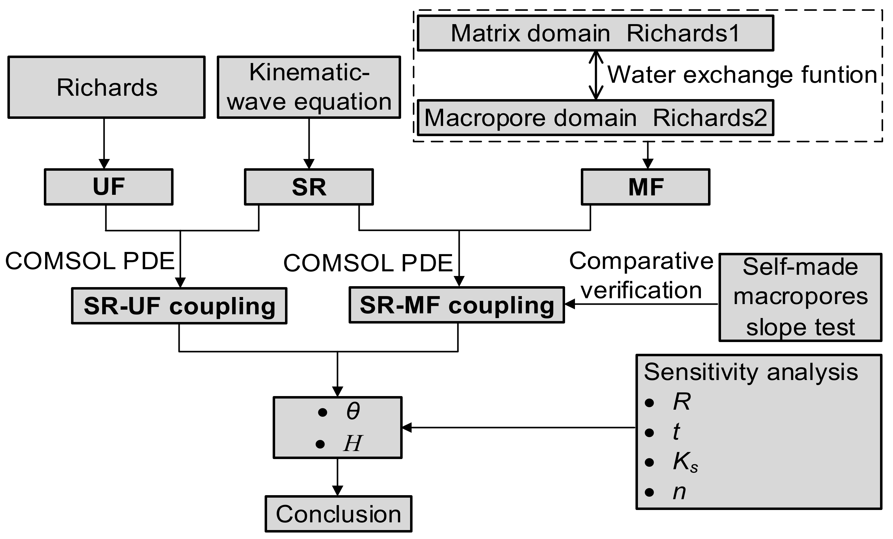
2.1. Framework

As shown in Figure 1, this paper divides infiltration into UF infiltration and MF infiltration. Firstly, the control equations of SR, UF, and MF were presented, and the coupled process based on a previous study [40] was introduced to build the SR and UF coupled model and the SR and MF coupled model, respectively. Then, the coupled equations were solved by COMSOL, and the feasibility of the model was verified by the self-made laboratory macropore slope test. Finally, a residual soil slope was taken as an example to evaluate the parameter sensitivity of water content and ponding depth, and results from the two coupled models were compared.

2.2. Theoretical Equations

2.2.1. SR Governing Equation

In 1871, Saint Venant proposed the equation of unsteady flow in open channels; however, this is only applicable to river channels and channels with a very gentle slope angle. For slopes with a large angle, the runoff water depth is usually very shallow, and Slope Runoff is greatly affected by microtopography. The complete Saint-Venant equations do not necessarily describe this particular flow well, and in existing research, the simplified form of the equations was usually used. The one-dimensional Saint Venant equation can be expressed by the kinematic wave equation [41], as shown in Equation (1):

$$\left\{\begin{array}{l}\frac{\partial H}{\partial t}+\frac{\partial q}{\partial x}=R\cos \phi -I\\ q=vH=\frac{1}{n}{H}^{\frac{5}{3}}{\sin }^{\frac{1}{2}}\phi \end{array}\right.$$

(1)

where t is time (s), v and H are the runoff velocity (m/s) and the runoff ponding depth (m), respectively, q is the single-width flow rate of slope (m²/s), R is the rainfall intensity (m/s), I is the infiltration rate (m/s), n is the slope surface roughness coefficient, and φ is the slope angle (°).

2.2.2. Rainfall Infiltration Equation

(1)

UF governing equation

When the macropores inside the slope are ignored, the water migration follows the traditional UF during rainfall. Assuming that the soil is homogeneous, the wetting front is parallel to the soil surface, and the two-dimensional infiltration process is expressed by a two-dimensional Richards equation [42], as shown in Equation (2):

$$C(h)\cdot \frac{\partial h}{\partial t}=\frac{\partial }{\partial x}\left(K(h)\frac{\partial h}{\partial x}\right)+\frac{\partial }{\partial z}\left(K(h)\frac{\partial h}{\partial z}+K(h)\right)$$

(2)

where h is the pressure head (m), C is specific water capacity (m⁻¹), and K is unsaturated water conductivity (m/s).

In unsaturated soil, C, K and effective saturation S_e are all variables related to water content θ or pressure head h, and are represented by the VG model [43], as shown in Equations (3)–(6):

$$C(h)=\frac{({\theta }_s-{\theta }_r)mn\alpha {\left|\alpha h\right|}^{n-1}}{{\left[1+{\left|\alpha h\right|}^n\right]}^{m+1}}$$

(3)

$$K=K_s{S}_e^l{[1-(1-S_e^{1/m}{)}^m]}^2$$

(4)

$$S_e=\frac{\theta -{\theta }_r}{{\theta }_s-{\theta }_r}$$

(5)

$$\theta (h)={\theta }_r+\frac{{\theta }_s-{\theta }_r}{{\left[1+{\left|\alpha h\right|}^n\right]}^m}$$

(6)

where θ_r is the residual water content, θ_s is saturated water content, K_s is the saturated water conductivity (m/s), α, n, m, and l are the fitting parameters of soil-water characteristic curve, and m = 1 − 1/n.

(2)

MF governing equation

When the macropores are considered, the water migration velocity at the macropore channel is faster than in other areas, and the wetting front is no longer regular. The dual permeability model is used to describe the movement. The dual permeability model assumes that the soil is composed of a matrix domain and macropore domain, and water can flow in both domains [43]. Figure 2 shows the simplified traditional UF and MF coupled model, where (a) is the traditional UF and (b) is MF. It can be seen that the macropore domain only accounts for a small part. When water flows downward, the infiltration rate between the two domains is significantly different. The migration velocity of the macropore domain is significantly higher than that of the matrix domain. The water in the two domains exchanges with each other, reflecting the imbalance of MF.

Water migration in the dual permeability model is described by two Richards equations. Each of them adds a water exchange term to couple the two domain equations, as shown in Equation (7):

$$\left\{\begin{array}{l}{C}_m\cdot \frac{\partial h_m}{\partial t}=\frac{\partial }{\partial x}\left(K_m\frac{\partial h_m}{\partial x}\right)+\frac{\partial }{\partial z}\left(K_m\frac{\partial h_m}{\partial z}+K_m\right)+\frac{{\Gamma }_{\omega }}{{\omega }_m}\\ C_f\cdot \frac{\partial h_f}{\partial t}=\frac{\partial }{\partial x}\left(K_f\frac{\partial h_f}{\partial x}\right)+\frac{\partial }{\partial z}\left(K_f\frac{\partial h_f}{\partial z}+K_f\right)-\frac{{\Gamma }_{\omega }}{{\omega }_f}\end{array}\right.$$

(7)

where h, C, and K have been described above, the subscripts m and f represent the matrix domain and macropore domain, respectively, ω_f is the proportion of macropore domain, taken as 0.05, ω_m = 1 − ω_f, and Γ_ω is the two-domain water exchange term (s⁻¹), as shown in Equation (8):

$${\Gamma }_{\omega }=\frac{\beta }{d^2}{r}_w{K}_a(h_f-h_m)$$

(8)

where β is the geometric shape factor of soil aggregates, which is taken as 3 for cuboid and 15 for sphere, d is the distance from the center of the granulation block to the edge of the macropore (m), taken as 0.01, and r_w is an empirical parameter and is set to 0.4.

In Equation (8), K_a is the hydraulic conductivity coefficient at the interface between the macropore domain and the matrix domain and is expressed by Equation (9):

$$K_a=0.5(K_f+K_m)$$

(9)

The relationship between other variables is shown in Equations (3)–(6). Since C and K are both variables related to pressure head h, Equations (2) and (7) are second-order nonlinear PDEs, which will be solved by numerical methods under certain assumptions.

2.2.3. Coupled Process

The slope is dry at the beginning of rainfall, and the upper surface is the flow boundary. When the slope is saturated, or the rainfall intensity is greater than the infiltration rate, the runoff occurs on the slope surface, and the upper surface boundary condition is transformed into the boundary of the pressure water head, which is determined according to the ponding depth. In view of the infiltration rate in Equation (1) is determined by the pressure water head and conductivity, in the same time step, Equations (1) and (7) are a fully coupled process formed by ponding depth and surface infiltration rate, and Equation (7) is coupled by Γ_ω internally. The coupled process based on the previous study [40] is shown as follows:

The infiltration solution of the n-1 time step is used to calculate the infiltration rate I, as shown in Equation (10):

$$\begin{array}{l}{I}_m={\left.K_m\frac{\partial h_m}{\partial N}\right|}_{\mathrm{s}\mathrm{u}\mathrm{r}\mathrm{f}\mathrm{a}\mathrm{c}\mathrm{e}} I_f={\left.K_f\frac{\partial h_f}{\partial N}\right|}_{\mathrm{s}\mathrm{u}\mathrm{r}\mathrm{f}\mathrm{a}\mathrm{c}\mathrm{e}}\\ I=w_m{I}_m+w_f{I}_f\end{array}$$

(10)

where N is the normal vector of the surface.

(a)

The I calculated above is substituted into Equation (1), and H is obtained.

(b)

The H obtained in step (a) is taken as the upper boundary condition of Equation (7), and then Equation (7) can be solved.

(c)

After solving Equation (7), I can be calculated according to step (a), and Equation (1) can be recalculated with I to solve H.

(d)

Equation (7) is solved by using H obtained in (c) as the upper boundary condition of Equation (7).

(e)

Steps (a)–(d) are repeated until Equations (1) and (7) converge.

(f)

Steps (a)–(e) are repeated until the end.

The SR and MF coupled model is obtained following the above process. For the coupled model of SR and UF, Equation (7) need to be replaced by Equation (2); there is no coupled term in the infiltration equation, and the infiltration rate I is still used by Equation (10), without distinction between the macropore domain and matrix domain; the Darcy equation can be used for calculation, and the solution process is relatively simple.

2.3. Model Test

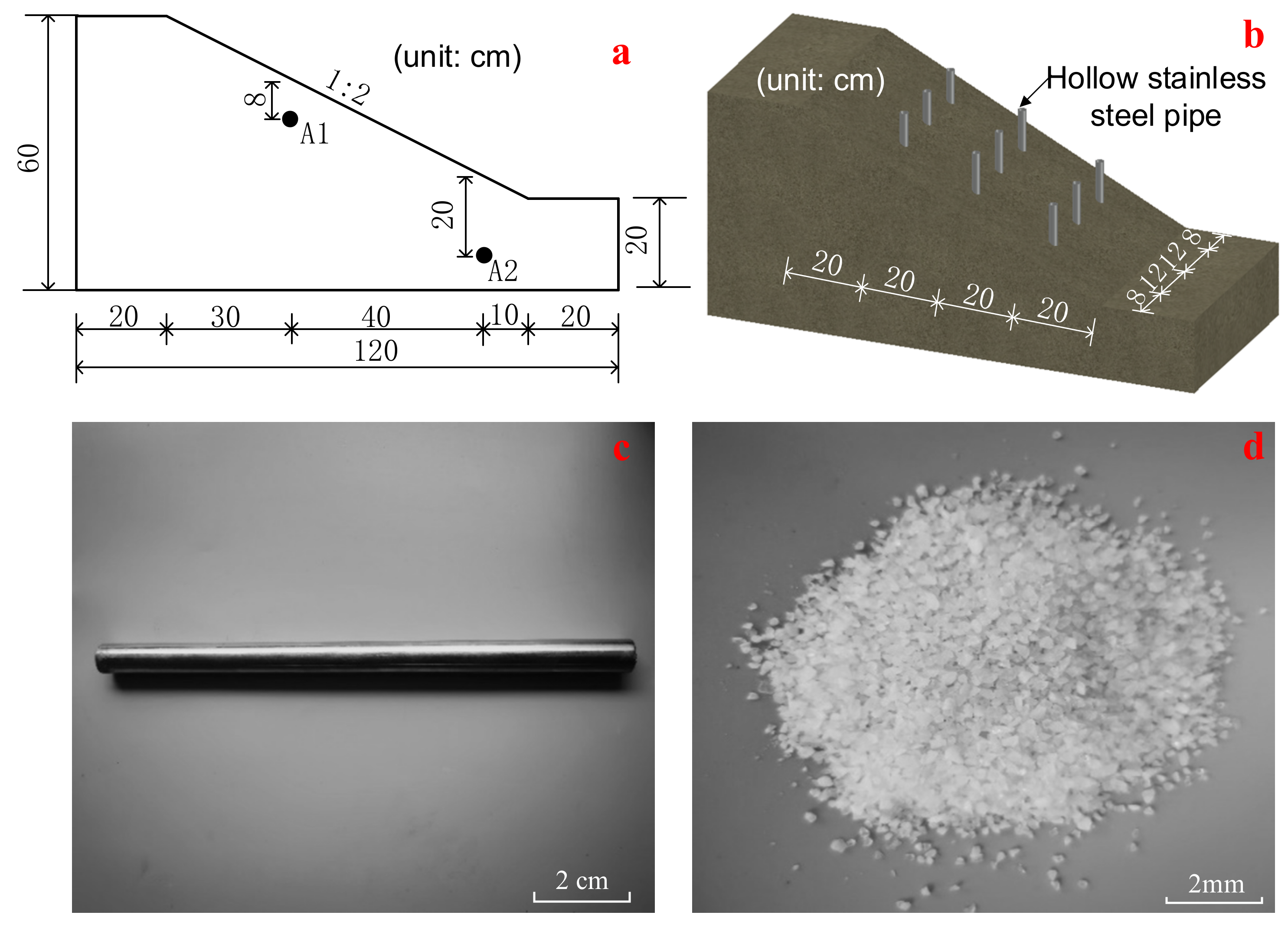
2.3.1. Test Slope Model

The soil for the test was derived from Section K103 + 160 of the Xia-Rong Expressway Extension Project (Zhangzhou, Fujian Province). The soil in the study area was sampled, and its natural moisture content was tested to be 10.2%. A total of 1 kg of soil was taken for the screening test. According to the results of particle analysis, it is judged that the undisturbed soil belongs to residual sandy cohesive soil. The permeability coefficient of the test soil is 4.9 cm/d, the compressive modulus is 5.12 MPa, and the cohesion and internal friction angle are 16.36 kPa and 36.4°, respectively.

In order to verify the effectiveness of the theoretical method, a laboratory macropore model test was designed. The results from the theoretical and experimental methods were compared. The test slope model is 120 cm long, including the slope top and toe, which are both 20 cm. The slope height is 60 cm, the height of the slope toe is 20 cm, and the slope ratio is 1:2. Two water content monitoring points, A₁ and A₂, were selected, and their specific locations are shown in Figure 3a.

Nine stainless-steel hollow pipes, which approximate macropores, were designed for this rainfall test. Three rows, with three pipes in each row, were arranged along the long and the short sides of the slope, respectively. The distance between neighboring pipes along the long side is 20 cm, and the distance between adjacent pipes along the short side is 12 cm, as shown in Figure 3b. These stainless-steel hollow pipes with a 2 cm diameter were inserted into the soil before filling. One of the pipes is shown in Figure 3c. After the filling, the quartz sand with a particle size of 2 mm, as shown in Figure 3d, is poured into the pipes [44]. Then, the steel pipes are pulled out slowly in an upward spiral way.

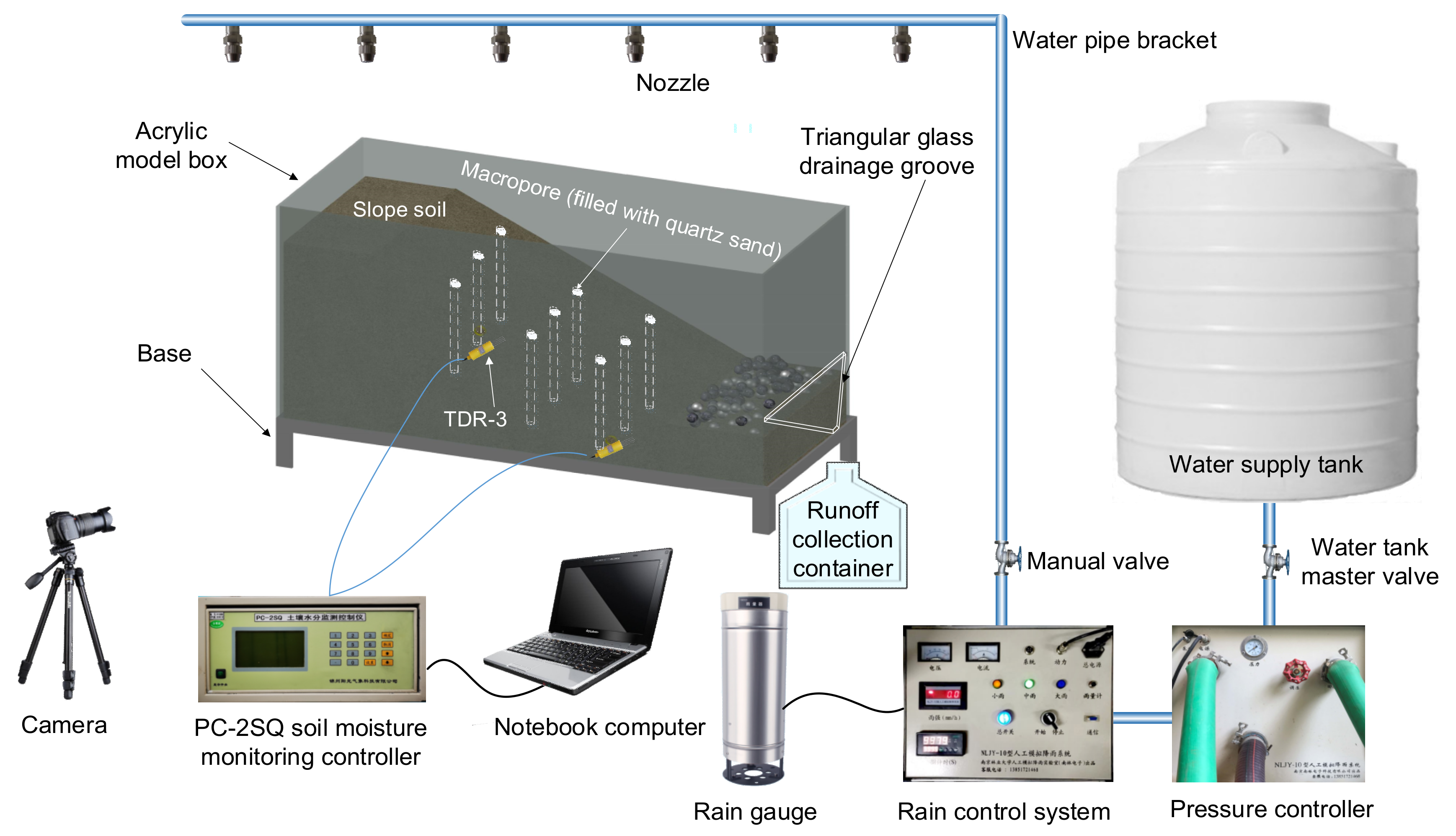
2.3.2. Testing Apparatus

The test apparatus is mainly composed of the main body of the model box, the base, the rainfall system, the data monitoring device, and the shooting device, as shown in Figure 4.

The main body of the model box is made of 8 mm thick acrylic transparent glass, which is used to support the soil filling of the slope. The long box is provided with two round holes with a diameter of 5 cm, which is used to allocate the water sensor. The short side (the outlet of the model box) is provided with a long hole with a width of 4 cm, which is used to connect the triangular glass drainage groove for collecting runoff.

The height of the base is 30 cm. The base is welded with an angle steel of 5 cm × 5 cm and 3 mm thickness. The base size matches the model box to ensure the model box is firm and reliable.

The rainfall system adopts NLJY-10 artificial simulated rainfall system developed by Nanjing Nanlin Electronic Technology Co., LTD, mainly composed of a sprinkler head, water pipe bracket, pressure control system, water supply tank, bucket rain gauge, and rainfall control system. The rainfall device is provided with six sprinkler points spaced at 2 m. Each sprinkler point contains three different sprinkler heads, and the nozzle diameter is 1.5 mm, 3.2 mm, and 5.0 mm, respectively, to simulate different rainfall intensities. The height of the sprinkler head is 6 m from the ground to ensure the uniformity of the rainfall. The water pipe bracket is mainly used to transport water and place the sprinkler head, and its layout is coordinated with the sprinkler head so that the effective rainfall area is not less than 12 m². The pressure control system is the main power of rainfall. The ball valve is adjusted by controlling the pressure of the water pump to adjust the rain strength. Usually, the control range of rainfall intensity is 1 mm/h–200 mm/h, and the pressure value corresponding to the current rainfall intensity will be displayed in the pressure control box. The water supply tank is mainly used for continuous water supply during rainfall to ensure abundant rainfall. A bucket rain gauge can monitor the change of rain intensity in real-time to control the rain intensity further [45]. The entire system is equipped with computer monitoring software that shows current rainfall intensity, pipe pressure, valve status, etc.

The data monitoring device includes soil water monitor and runoff velocity and accumulated runoff collection device. The soil water monitor is made by a PC-2SQ controller connected with a TDR-3 water content sensor (range 0~100% m3M-3, accuracy ± 2%). During the test, it is arranged in the hole reserved on the side of the model box, and the measurement process must be in close contact with the soil. The runoff velocity is measured by the staining method using KMnO₄ since the purplish-red KmnO₄ solution is highly differentiated. The runoff velocity is calculated by the time for the water flow to pass a certain distance on the slope surface. In this rainfall test, the locations with obvious runoff phenomena were selected to measure the flow velocity. First, a certain amount of KmnO₄ solution was dropped on the top of the slope with a rubber tip dropper. Then, the time for the purple water to reach the foot of the slope was manually recorded, and the maximum flow velocity on the surface was obtained. Multiply the maximum flow rate by the corresponding flow regime coefficient (take 0.75) to get the runoff rate [46]. According to this step, the runoff rate can be obtained at different times by measuring every 5 min. The accumulated runoff on the slope is collected in the container by the self-made triangular glass drainage groove, which is bonded to the outlet of the model box through glass glue.

The shooting device adopts a Nikon D7500 SLR camera, with a maximum pixel number of 20.51 million, which can effectively record the rainfall water infiltration process.

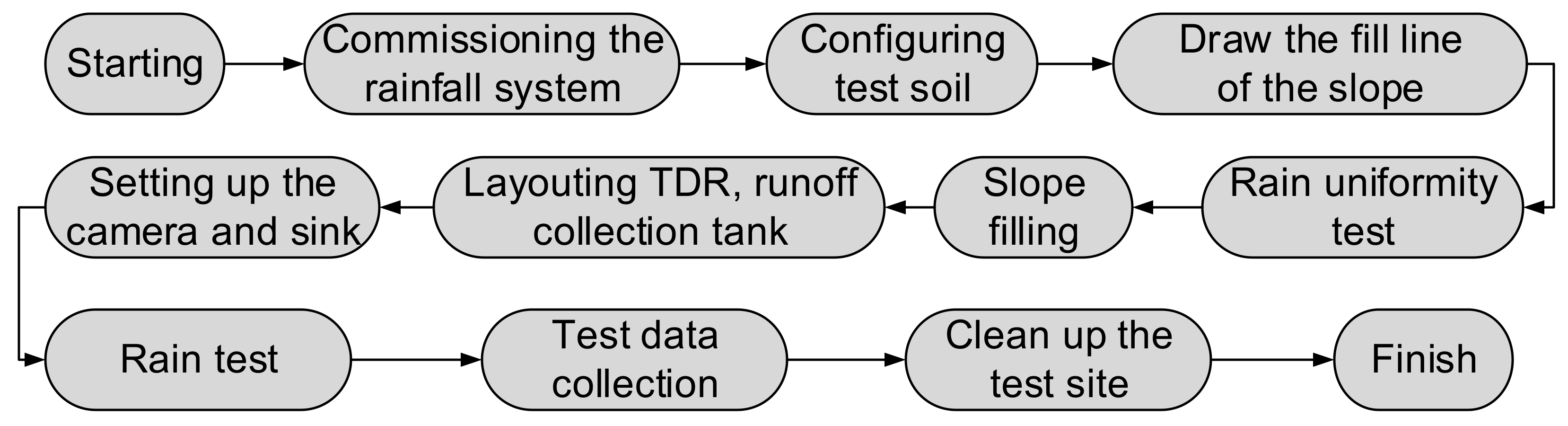
2.3.3. Test Procedure

Based on the above conditions, a laboratory macropore slope rainfall test was carried out. The rainfall intensity was 30 mm/h and the rainfall duration was 500 min. The main flow chart is shown in Figure 5.

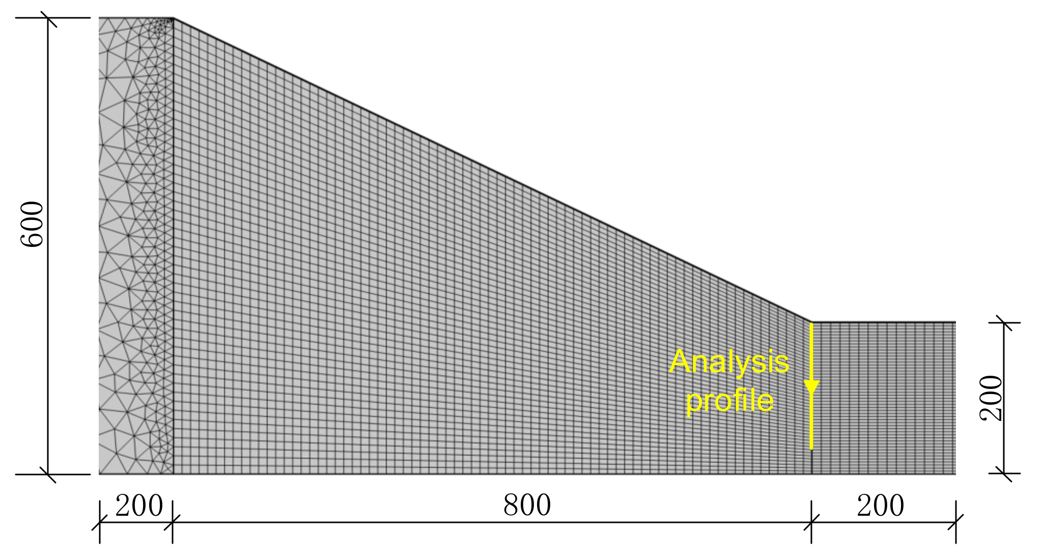
2.4. COMSOL PDE Calculation and Solution

COMSOL is a multi-physical field simulation software coupled with finite elements, of which the PDE interface under the mathematical branch can solve nonlinear PDEs. The PDE interface provides three application modes, including the coefficient form, general form, and weak form. In addition, the PDE can be customized by setting parameters, variables, and boundary conditions according to the needs of the research problem.

In this paper, coefficient form PDE is selected for modeling and calculation, and its basic form is Equation (11):

$$\left\{\begin{array}{ll}{e}_a\frac{{\partial }^{2}u}{\partial t^2}+d_a\frac{\partial u}{\partial t}+\nabla \cdot (-c\nabla u-\alpha u+\gamma )+\mathsf{\beta }\cdot \nabla u+\alpha u=f& \mathbf{in} \mathsf{\Omega }\\ \mathit{n}\cdot (c\nabla u+\alpha u-\gamma )=g-qu+h^T\mu & \mathbf{on} \partial \mathsf{\Omega }\\ 0=R& \mathbf{on} \partial {\mathsf{\Omega }}_c\\ u=r& \mathbf{on} \partial {\mathsf{\Omega }}_d\end{array}\right.$$

(11)

where u is a dependent variable, t is time, ∇ is the Hamiltonian operator, e_a, d_a, c, α, γ, and β coefficients are defined according to the control equations for the user, f, g, q, h, μ, R, and r are defined according to the boundary conditions for the user’s expression, Ω and ∂Ω are for calculating area and the boundary, and the boundary of n is outside the normal vector.

In the above equations, the first row solves the coefficient form PDEs on the domain Ω, and the rest are boundary condition equations. The second row is the Neumann boundary condition. The third and fourth rows are the Dirichlet boundary conditions, which are constraint boundary conditions.

Compared with other finite element software, COMSOL has a powerful multi-physics coupling function. Users can define variables and parameters flexibly, so it has certain advantages in solving complex equations. When using the PDE interface, various coefficients and expressions in the equations must be defined in advance. These coefficients and expressions can be custom parameters and functions of time and space coordinates and the dependent variable. After Equations (1), (2) and (7) are converted into coefficient form PDEs, the values of the coefficients and expressions are shown in

Table 1. Setting of coefficients and expressions in COMSOL PDE interface.

Coefficient	ea	da	c	α	γ	β	∇	f	u
Equation (1)	0	1	0	0	0	0	0	Rcosφ – I − ∂q/∂x	H
Equation (2)	0	C	K	0	0	0	∂(·)/∂x + ∂(·)/∂z	∂K/∂z	h
Equation (3)	0	Cm	Km	0	0	0	∂(·)/∂x + ∂(·)/∂z	∂K/∂z + Γω/(1 − ωf)	hm
	0	Cf	Kf	0	0	0	∂(·)/∂x + ∂( ·)/∂z	∂K/∂z − Γω/ωf	hf

.

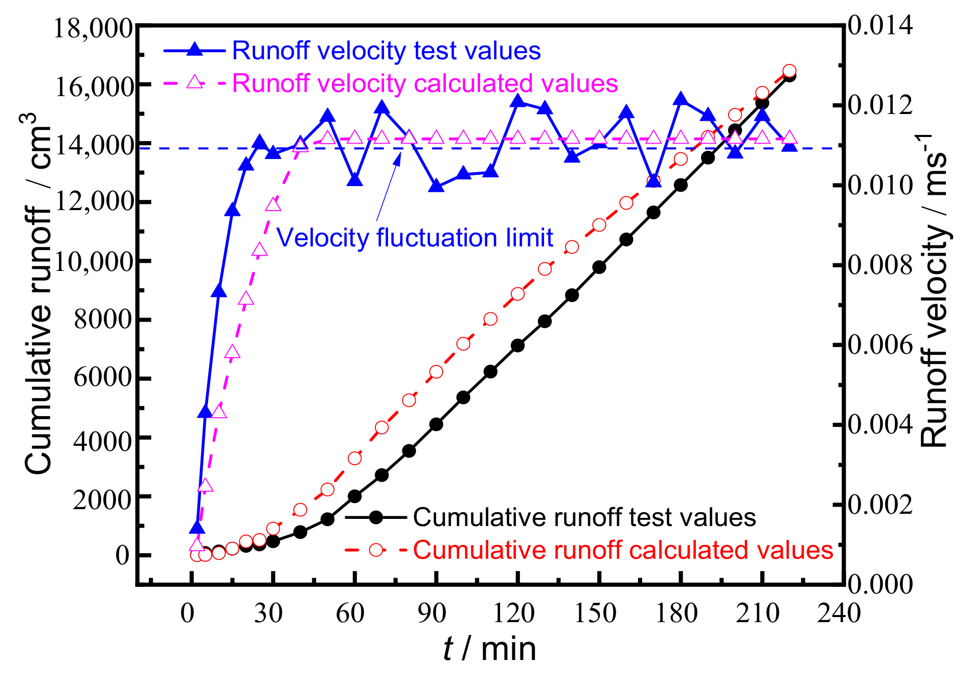
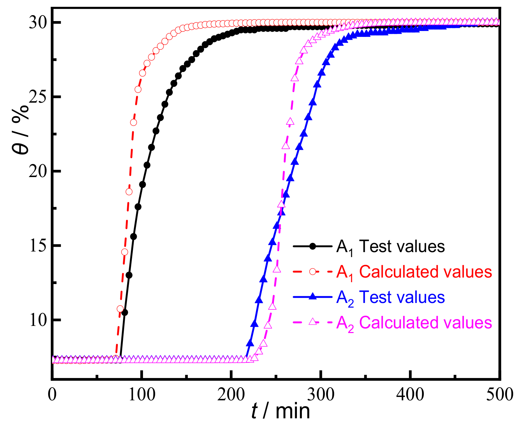
2.5. Model Validation

According to the geometric slope model in Figure 3a, a fully coupled model for Equations (1) and (7) is established based on COMSOL PDE, and the numerical solution results are compared with the above test values.

Figure 6 shows the comparison between the test values and calculated values of the water content of monitoring points A₁ and A₂. The variation trends of the test values and calculated values are roughly consistent, which remain unchanged at first and then increase rapidly. When the value is near the maximum value, the growth rate slows down and finally becomes stable. Specifically, the calculated and tested response times of monitoring point A₁ are 76 min and 81 min, respectively. The calculated response time is 6.2% earlier than the tested response time. The calculated time and tested response time of monitoring point A₂ are 236 min and 221 min, respectively. The calculated response time is 6.8% behind the test response time. The water content response time of calculated values and test values is nearly the same. The water content increases rapidly after the response time. When the soil at the monitoring point is close to saturation, the calculated values of water content at the same time are larger than the test values. When A₁ reaches saturation state, the corresponding time of test values and calculated values are 211 min and 156 min, respectively. When A₂ reaches saturation state, the corresponding time of test values and calculated values are 335 min and 296 min, respectively. The results show that it is easier to reach the saturation state under the numerical calculation condition. The main reason is that there is gas in the soil under the test condition, which can block the water infiltration, while the influence of gas is not considered under the calculation condition. In general, test results and calculation results of water content can form a reasonable verification.

Figure 7 compares the test and calculated values of cumulative runoff and runoff velocity on the slope. Cumulative runoff test values and calculated values both increase over time. From 0 to 30 min, the curves of the two almost overlap. After that, the growth rate of both curves increases. An inflection point appears, and the calculated value is slightly larger than the test value. This is because the absolute flatness of the slope cannot be guaranteed under the test conditions, resulting in a small amount of runoff delay. However, when the rainfall duration reaches 220 min, the test values and calculated values are 16,294 cm³ and 16,456 cm³, respectively, almost equal. The curves of the test and calculated values of runoff velocity show the same trend, which increases rapidly from 0 to 30 min. After 30 min, the calculated values level off and remain about 0.0112 m/s, while the test values fluctuate up and down. The velocity fluctuation limit is about 0.0109 m/s, which decreases by 2.68% compared with the calculated values due to certain friction on the test slope surface, resulting in the less average velocity of slope surface than the calculated values. On the whole, the test values of accumulated runoff and runoff velocity can be verified with the calculated values.

Figure 6 and Figure 7 show that self-made macropores using coarse quartz sand with a particle size of 2 mm can approximately simulate macropores. Moreover, the test results and numerical calculation results can be mutually verified, indicating that COMSOL PDE has high accuracy and feasibility in solving the coupled equations of SR and MF.

3. Case Analysis

The field investigation of the road residual soil slope along the S203 line in Fujian Province shows that the surface soil of the slope has a macropore structure. After continuous heavy rainfall in June 2016, the surface layer of the slope body has deformed, and the landslide scope has expanded, accompanied by slope collapse and mudslide as shown in Figure 8.

The slope height is 6 m, the width of the slope bottom is 12 m, the width of the slope top and toe is 2 m, the height of slope toe is 2 m, and the slope ratio is 1:2. The mesh is divided by mapping with a refined mesh size to improve the calculation accuracy. The whole model is divided into 5229 units and 459 boundary units, as shown in Figure 9.

The calculated boundary conditions are as follows: there is no flow boundary on two sides and the bottom of the rainfall infiltration model. When the actual rainfall time is less than the time when runoff occurs, the slope adopts a flow boundary. On the contrary, according to the iterative steps in Section 2.2.3, the ponding depth is taken as the boundary condition of the pressure head, and the initial condition is the fixed water content of 0.1. The boundary condition of the runoff equation is that the runoff velocity and ponding depth at the top of the slope are zero. The initial condition is that there is no runoff on the slope at the beginning of rainfall and the runoff velocity and ponding depth are zero.

The relationship between water content and suction is measured by quantitative filter paper, and the Isqcurvefit function in MATLAB is used to fit the VG model parameters to obtain the soil-water characteristic curve parameters. According to Highway Engineering Test Code, the variable head-test is used to measure the saturated conductivity of residual soil in the matrix domain, and the constant head permeability test is used to measure the saturated conductivity of residual soil in the macropore domain by filling coarse sand. The specific calculation parameters are shown in

Table 2. Slope calculation parameters.

Parameter	θr	θs	α (1/m)	n	l	Ks (cm/d)
Matrix domain	0.029	0.421	5.76	1.5	0.5	4.896
Macropores domain	0	0.5	10	2	0.5	2113.7

.

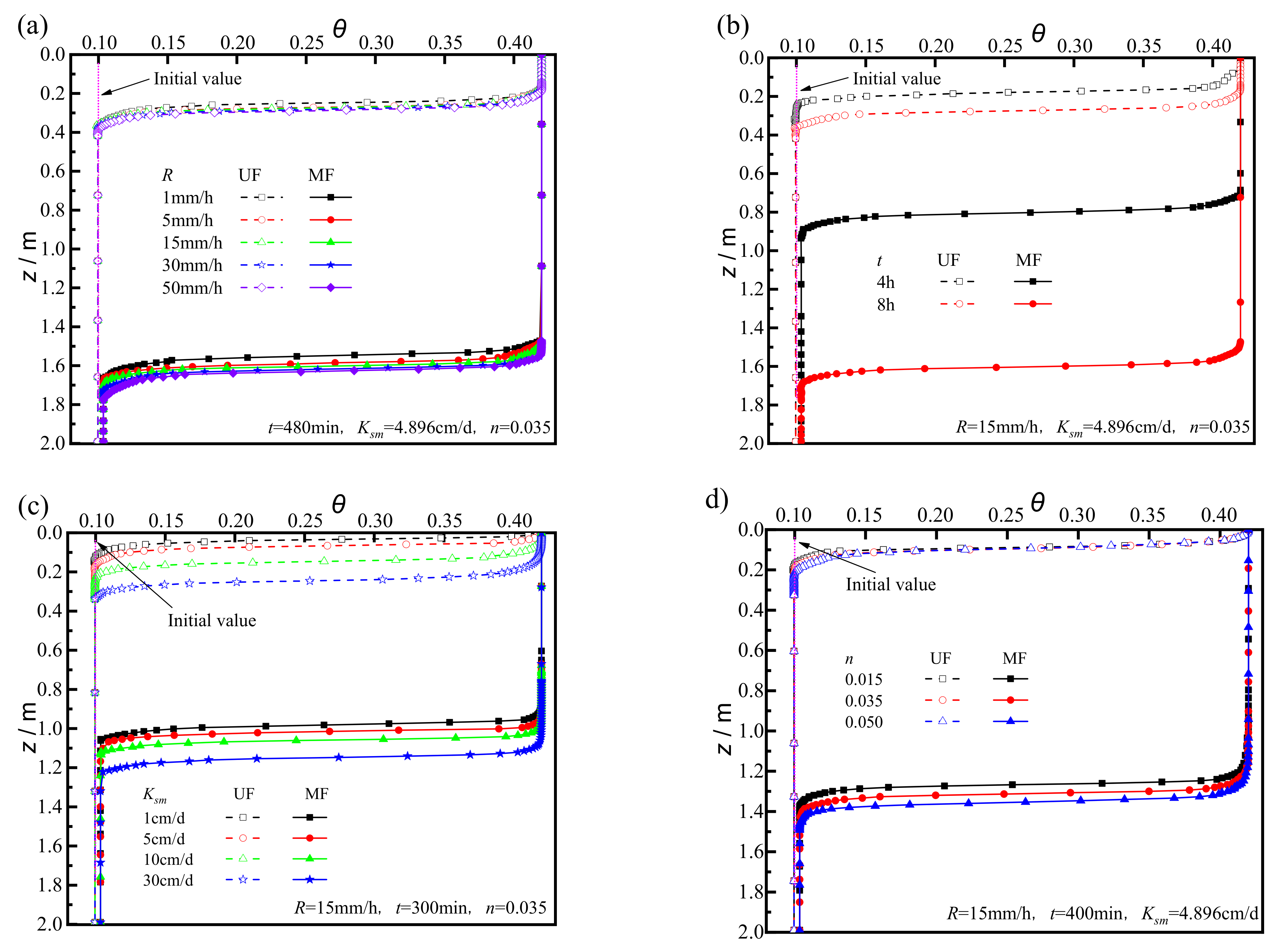
3.1. Water Content Distribution

Figure 10 is the water content distribution curve along with the profile under different influencing factors. The variation trends of the water content under different factors are similar, which are manifested in the surface soil at a certain depth in the saturated zone, the transition zone decreases, and the water content rapidly decreases to the initial value within a short depth range, reaching a wetting front depth. However, the degree of influence of each factor on the water field is different, and traditional UF and MF also show a big difference.

Figure 10a is the variation curve of water content with different rainfall intensities. The increase of rainfall intensity of MF is less than 5%, which is the same as the increase of wetting front depth of MF. The results indicate that the influence of rainfall intensity on water infiltration is weak. The main reason is that when SR is considered, the determination condition of the slope surface under rainfall is no longer the flow boundary but is affected by the ponding depth. However, there are significant differences in water infiltration between UF and MF under the same rainfall intensity. For example, when the rainfall intensity is 15 mm/h, the wetting front depth of UF and MF is 0.345 m and 1.685 m, respectively. The latter is almost five times the former because the water conductivity in the macropore domain is much higher than that in the matrix domain, which significantly promotes water infiltration.

Figure 10b shows the variation curves of water content with different rainfall duration. The UF saturated zone depth is about 0.146 m when the rainfall duration reaches 4 h, where the first inflection point appeared and the water content decreased rapidly to the initial value downward, and the wetting front depth is about 0.226 m. When the rainfall duration reaches 8 h, the water content curve is consistent with that at 4 h, but the saturated zone and wetting front depth increase to 0.246 m and 0.365 m, respectively, with an increase of 68.5% and 61.5%. When rainfall duration is 4 h, MF saturation zone and wetting front depths are 0.763 m and 0.882 m, respectively. When rainfall duration is 8 h, MF saturation zone and wetting front depths are 1.572 m and 1.698 m, an increase of 106.0% and 92.5%, respectively. The results show that, unlike the influence of rainfall intensity, the rainfall duration has a more significant impact on water infiltration both for UF or MF. The saturation zone and wetting front depth increase over rainfall duration. The reason is that when considering the Slope Runoff, the soil infiltration rate is not zero, even if the boundary is a pressure boundary. The slope surface still has a certain infiltration capacity, but the infiltration rate is less than the rainfall intensity. In addition, when the rainfall duration reaches 8 h, the saturated zone and wetting front depth of MF increased by 539.0% and 365.2%, respectively, indicating that the water infiltration depth has increased significantly considering macropores, consistent with the influence law of rainfall intensity.

Figure 10c shows the variation curve of water content with different saturated conductivities of the matrix domain K_sm. When the water conductivity is 1 cm/d, the maximum water content of UF surface soil is 0.419, which decreases rapidly along with the profile and reaches about 10 cm in the final wetting front depth. When the conductivity increases to 5 cm/d, 10 cm/d, and 30 cm/d, the topsoil is saturated, and the corresponding wetting front depth is 14 cm, 21 cm, and 33 cm, which increased by 40%, 50%, and 57.1%, respectively. The water content of MF advances deeper than that of UF. When the conductivity is 1 cm/d, 5 cm/d, 10 cm/d, and 30 cm/d, the saturation zone depths are 87 cm, 93 cm, 98 cm, and 105 cm, and the wetting front depth is 105 cm, 110 cm, 114 cm, and 122 cm, respectively. Both saturated zone and wetting front depth increase with the increase of water conductivity. However, the wetting front depth growth rate of UF is much higher than that of MF. For example, when the saturated conductivity increases from 5 cm/d to 10 cm/d, the wetting front depth growth rate of UF is 50%, while the MF is 3.6%, indicating that the UF is more sensitive to saturated conductivity than the MF. The reason is that the water conductivity K_sf of the macropore domain reaches 2113.7 cm/d (Table 2). According to K = w_mK_sm + w_fK_sf [43], the saturated conductivity of MF is mainly dominated by the macropores domain. Even if the conductivity of the matrix domain increases to the maximum value of 30 cm/d, the saturated conductivity growth rate of MF is still small, while that of UF is large.

Figure 10d shows the variation curves of water content with different roughness coefficients. The UF water content variation curves almost overlap when the roughness coefficients are 0.015, 0.035, and 0.050. The depth of the saturated zone on the slope surface is maintained at about 3 cm, and the wetting front depths are 18 cm, 20 cm, and 22 cm. It can be seen that the UF roughness coefficient has little effect on the water content of the slope, and only the wetting front depth increases slightly. The saturation zone depths corresponding to MF are 1.18 m, 1.22 m, and 1.26 m, and the wetting front depths are 1.33 m, 1.38 m, and 1.43 m. The growth rate of the water content response value is less than 4% for each increase of the above roughness coefficients, indicating that the slope roughness coefficient has little influence on the soil water content. The main reason is that the roughness coefficient is not directly related to the water field. The intermediate variable ponding depth affects the water field, but the water depth throughout the process is small, which is not enough to have a significant impact on the water field.

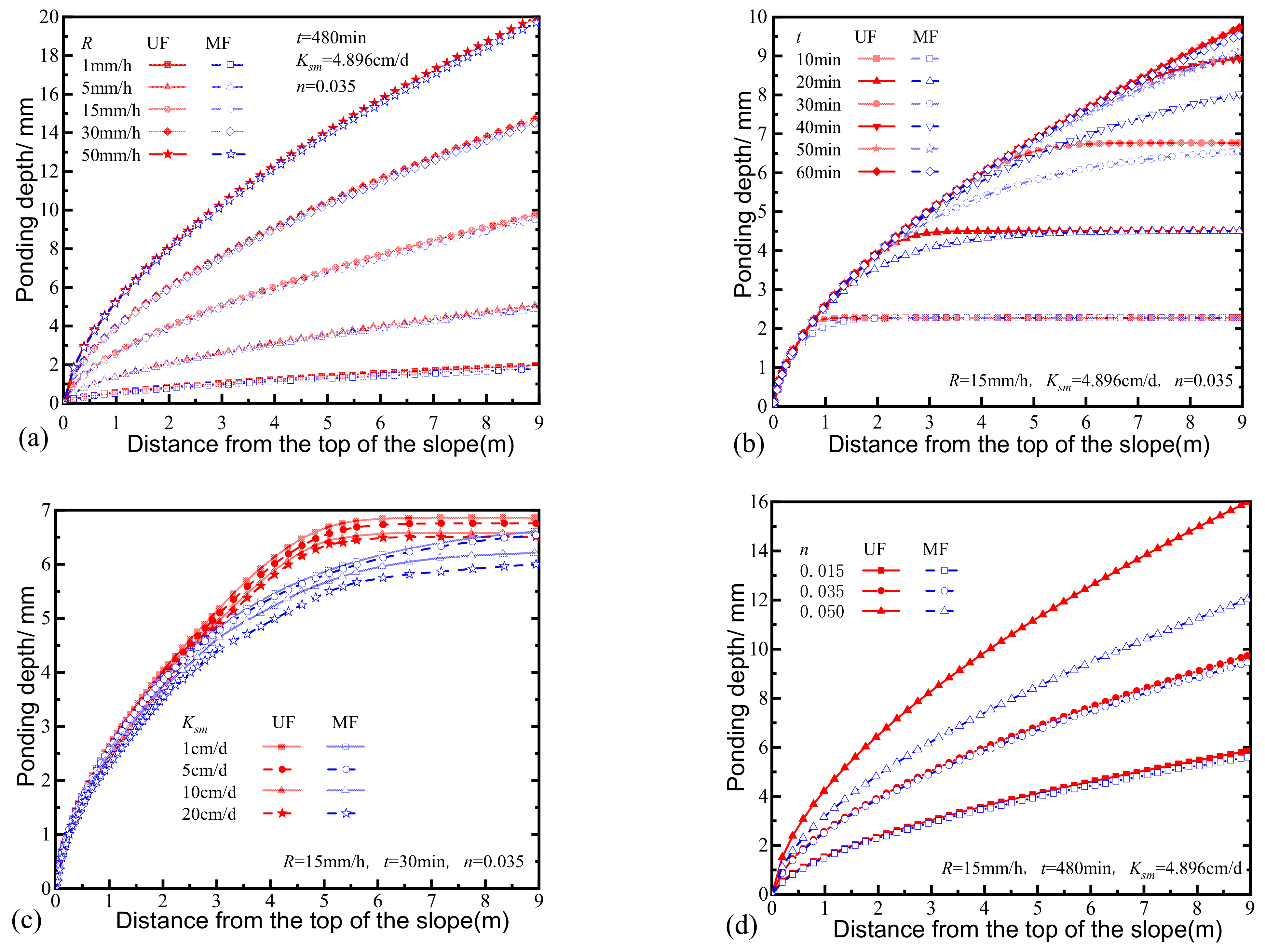
3.2. Ponding Depth Distribution

Figure 11 shows the distribution curves of ponding depth along the slope with different influencing factors. Figure 11a shows the influence of rainfall intensity. It can be seen that the ponding depth at any point on the slope increases significantly with the increase of rainfall intensity. For example, when the rainfall intensity is 1 mm/h, 5 mm/h, 15 mm/h, 30 mm/h, and 50 mm/h, the maximum ponding depth of UF is 2.053 mm, 4.762 mm, 9.813 mm, 15.886 mm, and 20.177 mm, respectively, with an increasing rate of 102.3%, 98.4%, 63.3%, and 27.9%, respectively. In addition, along the slope surface, the ponding depth gradually increases, reaching the maximum value at the foot of the slope, but the growth rate keeps decreasing. As shown in Figure 11a, the ponding depth in the middle of the slope has reached about 66% of the maximum value at five rainfall intensities, indicating an increase of more than 50% on half of the slope. The variation pattern of the MF ponding depth is basically the same as that of UF. For example, at a rain intensity of 15 mm/h, the maximum ponding depth of MF decreases by only 0.013 mm (1.62%) compared with UF. The above results show that there is no significant difference in the ponding depth of the slope surface under the two seepage modes, and there is only a slight decrease in the ponding depth of MF compared with that of UF.

Figure 11b shows the variation curves of the ponding depth with rainfall durations from 0 to 60 min. It can be seen that when the rainfall duration reaches 10 min, the ponding depth increases rapidly along the slope for both seepage modes. When a certain position is reached, there is an inflection point where the ponding depth does not increase and stabilizes at 2.25 mm. The difference is that UF reaches its maximum value after 1.18 m from the top of the slope, while MF reaches its maximum value at 2.14 m, and then enters the stable area. This result indicates that it is easier for UF to reach a stable state than MF. When the rainfall duration reaches 20 min, the ponding depth shows a similar variation pattern, but the maximum ponding depths of UF and MF are no longer the same, which are 4.505 mm and 4.503 mm, respectively, and the depth of MF is 0.04% lower than that of UF. In addition, the maximum ponding depths are 3.33 m and 5.70 m, respectively, and the distance is further increased. When the rainfall duration reaches 30 min, UF reaches a maximum ponding depth of 6.757 mm after 6.28 m, while MF reaches the maximum ponding depth of 6.534 mm at the foot of the slope, with a 3.30% decrease compared with UF. After 40 min of rainfall, the maximum ponding depths of UF and MF at the foot of the slope are 8.931 mm and 8.016 mm, respectively. MF is 10.24% smaller than UF, and there is no stable ponding zone at this time. When the rainfall duration reaches 50 min, the maximum values of MF and UF increase to 9.708 mm and 9.084 mm, respectively, and MF decreases by 6.43% compared with UF. When the rainfall duration reaches 60 min, the maximum ponding depth of UF is 9.726 mm, which barely increases any more, while the maximum value of MF increases to 9.527 mm, which is 2.05% lower than that of UF. In this paper, the slope length is 8.944 m. When the rainfall duration is less than 30 min, a stable area with zero growth rate of ponding depth appears on the slope. When the rainfall duration is more than 30 min, the stable area disappears, and the ponding depth grows slowly along the slope surface. It can be predicted that the stable area will always exist when the length of the slope is larger or even infinite, and its length will decrease with the increase of rainfall duration. In addition, increasing the rainfall duration can increase the ponding depth near the foot of the slope, but the depth at each point on the slope does not increase after 60 min. This result indicates that there is a limit to the influence of rainfall duration on the ponding, and the ponding depth will not change at the later stage under a long-lasting rainfall.

The influence of rainfall duration on the ponding depth of UF and MF is also different. When the duration increases from the initial time to 60 min with a variance of 10 min, the maximum ponding depth of MF decreases by 0%, 0%, 0.04%, 3.30%, 10.24%, 6.43%, and 2.05%, respectively. The length of the stable area is smaller than UF. UF and MF are considerably in ponding characteristics at the early stage of rainfall. After 60 min, their ponding depth curves are highly consistent, and in general, is easier to achieve stable water accumulation in UF than MF.

Figure 11c shows the variation curves of ponding depth at different saturated conductivity when the rainfall duration reaches 30 min. It can be seen that when the conductivity is 1 cm/d, the ponding depth of UF increases gradually along the slope, reaching a maximum of 6.86 mm at a distance of 6.1 m from the top of the slope, which then enters the stable area. When the conductivity is 5 cm/d, 10 cm/d, and 30 cm/d, the curves have a similar variation pattern and enter the stable area at about 6.1 m. However, the maximum value of the water depth of the slope surface decreases slightly with the increase of conductivity. For example, when the conductivity is 5 cm/d, 10 cm/d, and 20 cm/d, the corresponding ponding depth is 6.76 mm, 6.58 mm, and 6.51 mm. The variation pattern of ponding depth in MF slope is the same as that of conductivity. The main reason is that with the increase of conductivity, more water infiltrates into the slope body, making the ponding depth in the MF slope area smaller. However, there is no stable area in the variation curve of MF. The ponding depth gradually increases along the slope, indicating that it is more difficult for MF water to reach a stable state in the downslope area than UF, which is consistent with the influence law of rainfall duration.

Figure 11d shows the variation curves of ponding depth with different roughness coefficients. It can be seen that the variation trend along the slope is the same as above. When the roughness coefficients are 0.015, 0.035, and 0.050, the maximum ponding depths of UF are 5.85 mm, 9.73 mm, and 15.99 mm, respectively, with an increase of 66.3% and 64.3%. Under MF, the maximum ponding depths are 5.60 mm, 9.46 mm, and 12.02 mm, increasing 68.9% and 27.1%. It can be seen that ponding depth increases significantly with the increase of roughness coefficient, mainly because the more significant roughness coefficient increases the blocking effect of water flow on the slope, resulting in increasing water accumulation. In addition, when the roughness coefficient is 0.015 and 0.035, UF’s ponding depth only increases 4.5% and 2.9% compared with MF. When the roughness coefficient is 0.050, the increase is 33.0%. This result indicates that when the roughness coefficient is small, the ponding depths of UF and MF are almost the same. On the contrary, when the roughness coefficient reaches a specific value, it is difficult for the water to be lost along the slope in a short time, and there is enough time for infiltration along the macropores channels, making the ponding depth of MF significantly smaller than UF.

4. Discussion

A dual permeability model was used to describe the water migration in the macropore slope. The UF process was described by the Richards equation. Based on the kinematic-wave equation, the coupled models of SR and MF and SR and UF were established by the coupled terms of infiltration rate and ponding depth, respectively. The numerical solutions of the two coupled models were achieved by the COMSOL PDE finite element method. In addition, the validity of the numerical model and the accuracy of the algorithm were verified by the laboratory test model of a self-made macropore slope. Finally, the variation characteristics of slope water content and slope surface ponding depth of two coupled models with different influencing factors were quantitatively analyzed, and the main conclusions are as follows:

(1)

The coupled model of Slope Runoff and infiltration solved by the COMSOL has high accuracy, which can be mutually verified with the experimental results. The influence of rainfall intensity on the water infiltration of UF and MF is minimal when runoff is considered, which is quite different from the result with the slope as the flow boundary when SR is not considered. With a longer rainfall duration, the depth of the saturated zone and wetting front increases.

(2)

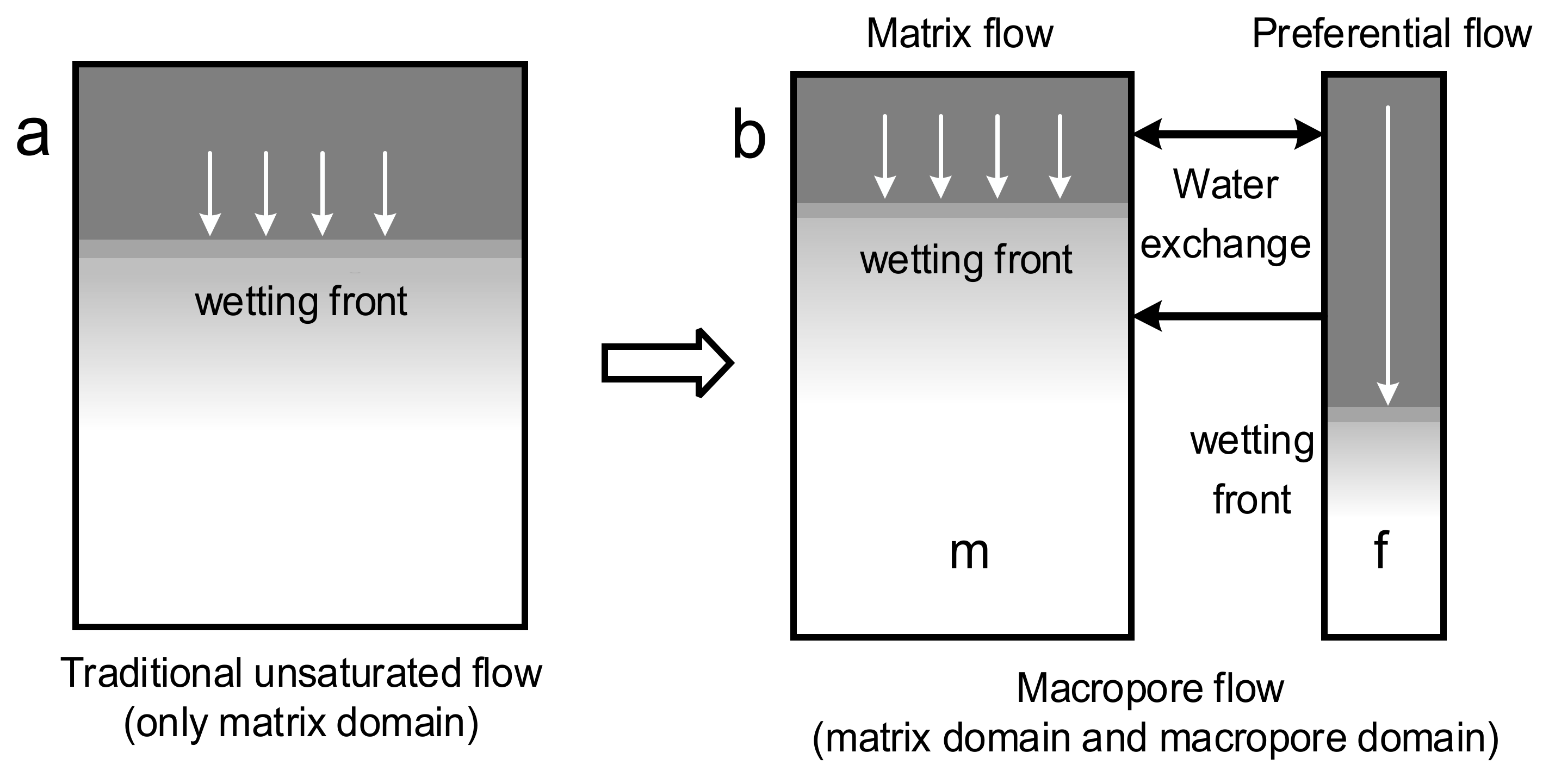
Permeability has a positive effect on the infiltration results, while the slope roughness coefficient has no direct relationship with the infiltration equation, thus having a weak effect on water infiltration. By comparing UF and MF, it is found that the depth of the saturation zone and wetting front of MF is remarkably higher than that of UF, which is mainly due to the high conductivity of the macropore channel. Therefore, macropores and their effects on the water infiltration depth should not be ignored when they exist in a slope.

(3)

Rain intensity has a significant influence on ponding depth in slope areas. When the rain intensity increases, the ponding depth will rise, but the length of the stable area will be reduced. However, the difference between UF and MF ponding depth is not apparent. Rainfall duration may affect the ponding depth only when the rainfall duration is small, and the ponding depth is positively correlated with the rainfall duration. In addition, with a shorter duration, the stable area of the slope becomes longer. The difference in ponding depth between UF and MF increased first and then decreased with rainfall duration, and they were almost the same eventually.

(4)

With the increase of saturated conductivity, the ponding depth decreased slightly, but the water depth of MF increased successively along the slope, while a stable area appeared in UF. Compared with UF, the ponding in MF slope was more difficult to reach a stable state. Ponding depth increases significantly with the increase of roughness coefficient. When the roughness coefficient is small, UF and MF have no significant difference. When the roughness coefficient reaches a certain level, the depth of MF ponding is significantly less than that of UF. The reason is that it is difficult to drain along the slope in a short period, and there is enough time for infiltration along the macropores channels.

(5)

In the actual situation, the SR is generated after a certain period of rainfall, and the critical time for runoff must be calculated. The boundary conditions of the slope surface should be determined according to the relationship between the rainfall duration and the critical time. Considering that the rainfall type in this study is heavy rainfall, the slope generates runoff in a short period, and the critical time of the runoff is ignored, making this study deviate from the actual situation. Therefore, the water infiltration depth should be investigated in future studies.

References

- Clague, J.; Stead, D. Landslides: Types, Mechanisms and Modeling; Cambridge University Press: Cambridge, UK, 2012. [Google Scholar]
- Lazzari, M.; Piccarreta, M.; Ray, R.; Manfreda, S. Modeling Antecedent Soil Moisture to Constrain Rainfall Thresholds for Shallow Landslides Occurrence. In Landslides: Investigation and Monitoring; IntechOpen: London, UK, 2020; pp. 1–32. [Google Scholar] [CrossRef]
- Lazzari, M.; Piccarreta, M.; Manfreda, S. The role of antecedent soil moisture conditions on rainfall-triggered shallow landslides. Nat. Hazards Earth Syst. Sci. 2018, 1–11. [Google Scholar] [CrossRef] [Green Version]
- Lazzari, M.; Piccarreta, M.; Capolongo, D. Landslide Triggering and Local Rainfall Thresholds in Bradanic Foredeep, Basilicata Region (Southern Italy). In Landslide Science and Practice; Springer: Berlin/Heidelberg, Germany, 2013. [Google Scholar] [CrossRef]
- Sun, L.; Ma, B.; Pei, L.; Zhang, X.; Zhou, J. The relationship of human activities and rainfall-induced landslide and debris flow hazards in Central China. Nat. Hazards 2021, 9, 147–169. [Google Scholar] [CrossRef]
- Springman, S.; Thielen, A.; Kienzler, P.; Friedel, S. A long-term field study for the investigation of rainfall-induced landslides. Geotechnique 2013, 63, 1177–1193. [Google Scholar] [CrossRef]
- Mukhlisin, M.; Taha, M.; Kosugi, K. Numerical analysis of effective soil porosity and soil thickness effects on slope stability at a hillslope of weathered granitic soil formation. Geosci. J. 2008, 12, 401–410. [Google Scholar] [CrossRef]
- Xie, M.; Esaki, T.; Cai, M. A time-space based approach for mapping rainfall-induced shallow landslide hazard. Environ. Geol. 2004, 46, 840–850. [Google Scholar] [CrossRef]
- Collins, B.; Znidarcic, D. Stability analyses of rainfall induced landslides. J. Geotech. Geoenviron. Eng. 2004, 130, 362–372. [Google Scholar] [CrossRef]
- Liu, J.; Yang, C.; Gan, J.; Liu, Y.; Liu, W.; Qiang, X. Stability analysis of road embankment slope subjected to rainfall considering runoff-unsaturated seepage and unsaturated fluid–solid coupling. Int. J. Civ. Eng. 2017, 15, 865–876. [Google Scholar] [CrossRef] [Green Version]
- Chiu, Y.; Chen, H.; Yeh, K. Investigation of the influence of rainfall runoff on shallow landslides in unsaturated soil using a mathematical model. Water 2019, 11, 1178. [Google Scholar] [CrossRef] [Green Version]
- Yang, Y.; Bao, H.; Peng, T. Verification and analysis of meteorological early warning of geological hazards during precipitation of Typhoon “MEGI”. Torrential Rain Disasters 2019, 38, 221–228. [Google Scholar]
- Cuomo, S.; Sala, M. Rainfall-induced infiltration, runoff and failure in steep unsaturated shallow soil deposits. Eng. Geol. 2013, 162, 118–127. [Google Scholar] [CrossRef]
- Kean, J.; McCoy, S.; Tucker, G.; Staley, D.; Coe, J. Runoff-generated debris flows: Observations and modeling of surge initiation, magnitude, and frequency. J. Geophys. Res. Earth Surf. 2013, 118, 2190–2207. [Google Scholar] [CrossRef]
- Wei, Z.; Shang, Y.; Yu, Z.; Pan, P.; Jiang, Y. Rainfall threshold for initiation of channelized debris flows in a small catchment based on in-site measurement. Eng. Geol. 2016, 217, 23–34. [Google Scholar] [CrossRef]
- Hua, Z.; Feng, Z.; Ke, S.; Mi, Y. A Surface and Subsurface Model for the Simulation of Rainfall Infiltration in Slopes. In IOP Conference Series: Earth and Environmental Science International Symposium on Geohazards and Geomechanics, Proceedings of the International Symposium on Geohazards and Geomechanics (ISGG2015), Warwick, UK, 10–11 September 2015; IOP Publishing: London, UK, 2015. [Google Scholar]
- Tian, D.; Zheng, H.; Liu, D. A 2D integrated FEM model for surface water–groundwater flow of slopes under rainfall condition. Landslides 2016, 14, 577–593. [Google Scholar] [CrossRef]
- Singh, V.; Bhallamudi, S. Conjunctive surface-subsurface modeling of overland flow. Adv. Water Resour. 1998, 21, 567–579. [Google Scholar] [CrossRef]
- Morita, M.; Yen, B. Modeling of conjunctive two-dimensional surface-three-dimensional subsurface flows. J. Hydraul. Eng. 2002, 128, 184–200. [Google Scholar] [CrossRef]
- Tong, F.; Tian, B.; Liu, D. A coupling analysis of Slope Runoff and infiltration under rainfall. Rock Soil Mech. 2008, 4, 1035–1040. [Google Scholar]
- Tian, D.; Liu, D. A new integrated surface and subsurface flows model and its verification. Appl. Math. Model. 2011, 35, 3574–3586. [Google Scholar] [CrossRef]
- Muntohar, A.; Liao, H. Rainfall infiltration: Infinite slope model for landslides triggering by rainstorm. Nat. Hazards 2010, 54, 967–984. [Google Scholar] [CrossRef]
- Han, T.; Su, Y.; Zhang, Y. Coupling analysis of rainfall infiltration and Slope Runoff in two-layered slope. Adv. Eng. Sci. 2020, 52, 145–152. [Google Scholar]
- HA, L.; Johnson, J. Infiltration on sloping terrain and its role on runoff generation and slope stability. J. Hydrol. 2018, 561, 584–597. [Google Scholar] [CrossRef]
- Johnson, J.; Loáiciga, H. Coupled infiltration and kinematic-wave runoff simulation in slopes: Implications for slope stability. Water 2017, 9, 327. [Google Scholar] [CrossRef] [Green Version]
- Tian, D.; Liu, D.; Zheng, H.; Wang, S. Numerical simulation of drain on landslide surface under rainfall condition. Rock Soil Mech. 2011, 32, 1255–1261. [Google Scholar]
- Liu, J.; Liu, Y. A preliminary study of rainfall infiltration on the slope using a new coupled procedure of overland runoff and unsaturated water-gas two phases seepage model. Appl. Mech. Mater. 2013, 2685, 221–226. [Google Scholar] [CrossRef]
- Bouchemella, S.; Seridi, A.; Alimi-Ichola, I. Numerical simulation of water flow in unsaturated soils: Comparative study of different forms of Richards’s equation. Eur. J. Environ. Civ. Eng. 2015, 19, 1–26. [Google Scholar] [CrossRef]
- Shigorina, E.; Rüdiger, F.; Tartakovsky, A.; Sauter, M.; Kordilla, J. Multiscale smoothed particle hydrodynamics model development for simulating preferential flow dynamics in fractured porous media. Water Resour. Res. 2020, 57, e2020WR027323. [Google Scholar] [CrossRef]
- Wissmeier, L.; Barry, D. Simulation tool for variably saturated flow with comprehensive geochemical reactions in two- and three-dimensional domains. Environ. Model. Softw. 2011, 26, 210–218. [Google Scholar] [CrossRef]
- Sun, X.; Luo, H.; Kenichi, S. A coupled thermal–hydraulic–mechanical–chemical (THMC) model for methane hydrate bearing sediments using COMSOL Multiphysics. J. Zhejiang Univ. Sci. A 2018, 19, 600–623. [Google Scholar] [CrossRef]
- Kong, X.; Wang, E.; Liu, Q. Dynamic permeability and porosity evolution of coal seam rich in CBM based on the flow-solid coupling theory. J. Nat. Gas Sci. Eng. 2017, 40, 61–71. [Google Scholar] [CrossRef]
- Xu, X.; Jian, W.; Wu, N. Influence of repeated wetting cycles on shear properties of natural residual soil. China J. Highw. Transp. 2017, 30, 33–40. [Google Scholar]
- Chertkov, V.; Ravina, I. Modeling the crack network of swelling clay soils. Soil Sci. Soc. Am. J. 1998, 62, 1162–1171. [Google Scholar] [CrossRef]
- Hendrickx, J.; Flury, M. Uniform and Preferential Flow Mechanisms in the Vadose Zone. In Conceptual Models of Flow and Transport in the Fractured Vadose Zone; NAP: Pittsburgh, PA, USA, 2001. [Google Scholar]
- Jarvis, N. A review of non-equilibrium water flow and solute transport in soil macropores: Principles, controlling factors and consequences for water quality. Eur. J. Soil Sci. 2007, 58, 523–546. [Google Scholar] [CrossRef]
- Bogaard, T.; Greco, R. Landslide hydrology: From hydrology to pore pressure. Wiley Interdiscip. Rev. Water 2016, 3, 439–459. [Google Scholar] [CrossRef]
- Mencaroni, M.; Dal Ferro, N.; Radcliffe, D.E.; Morari, F. Preferential solute transport under variably saturated conditions in a silty loam soil: Is the shallow water table a driving factor? J. Hydrol. 2021, 602, 126733. [Google Scholar] [CrossRef]
- Wang, R.; Dong, Z.; Zhou, Z.; Wang, N.; Xue, Z.; Cao, L. Effect of vegetation patchiness on the subsurface water distribution in abandoned farmland of the Loess Plateau, China. Sci. Total Environ. 2020, 746, 141416. [Google Scholar] [CrossRef] [PubMed]
- Zhang, P.; Liu, D.; Zheng, H. Coupling numerical simulation of Slope Runoff and infiltration under rainfall conditions. Rock Soil Mech. 2004, 25, 109–113. [Google Scholar]
- Lu, Z.; Tung, Y.; Ng, C.; Tang, W. International Symposium on Environmental Hydraulics & Sustainable Water Management1, Environmental Hydraulics. In Sensitivity and Uncertainty Analyses of Coupled Surface-Subsurface Flow Model on Steep Slopes; Taylor & Francis: London, UK, 2004. [Google Scholar]
- Richard, L. Capillary conduction of liquids through porous mediums. Physics 1931, 1, 318–333. [Google Scholar] [CrossRef]
- Gerke, H.; Van Genuchten, M. A dual-porosity model for simulating the preferential movement of water and solutes in structured porous media. Water Resour. Res. 1993, 29, 305–319. [Google Scholar] [CrossRef]
- Kohne, J.; Mohanty, B. Water flow processes in a soil column with a cylindrical macropore: Experiment and hierarchical modeling. Water Resour. Res. 2005, 41, e2004WR003303. [Google Scholar] [CrossRef] [Green Version]
- Dai, Y.; Jiang, J.; Gu, X.; Zhao, Y.; Ni, F. Sustainable Urban Street Comprising Permeable Pavement and Bioretention Facilities: A Practice. Sustainability 2020, 12, 8288. [Google Scholar] [CrossRef]
- Ni, S.; Zhang, D.; Feng, S. Quantitative relationship between hydraulics parameters and soil erosion rate on remolded soil slopes with different textures. Acta Pedol. Sin. 2019, 56, 1336–1346. [Google Scholar]