
A Multigrid Dynamic Bidirectional Coupled Surface Flow Routing Model for Flood Simulation


Abstract
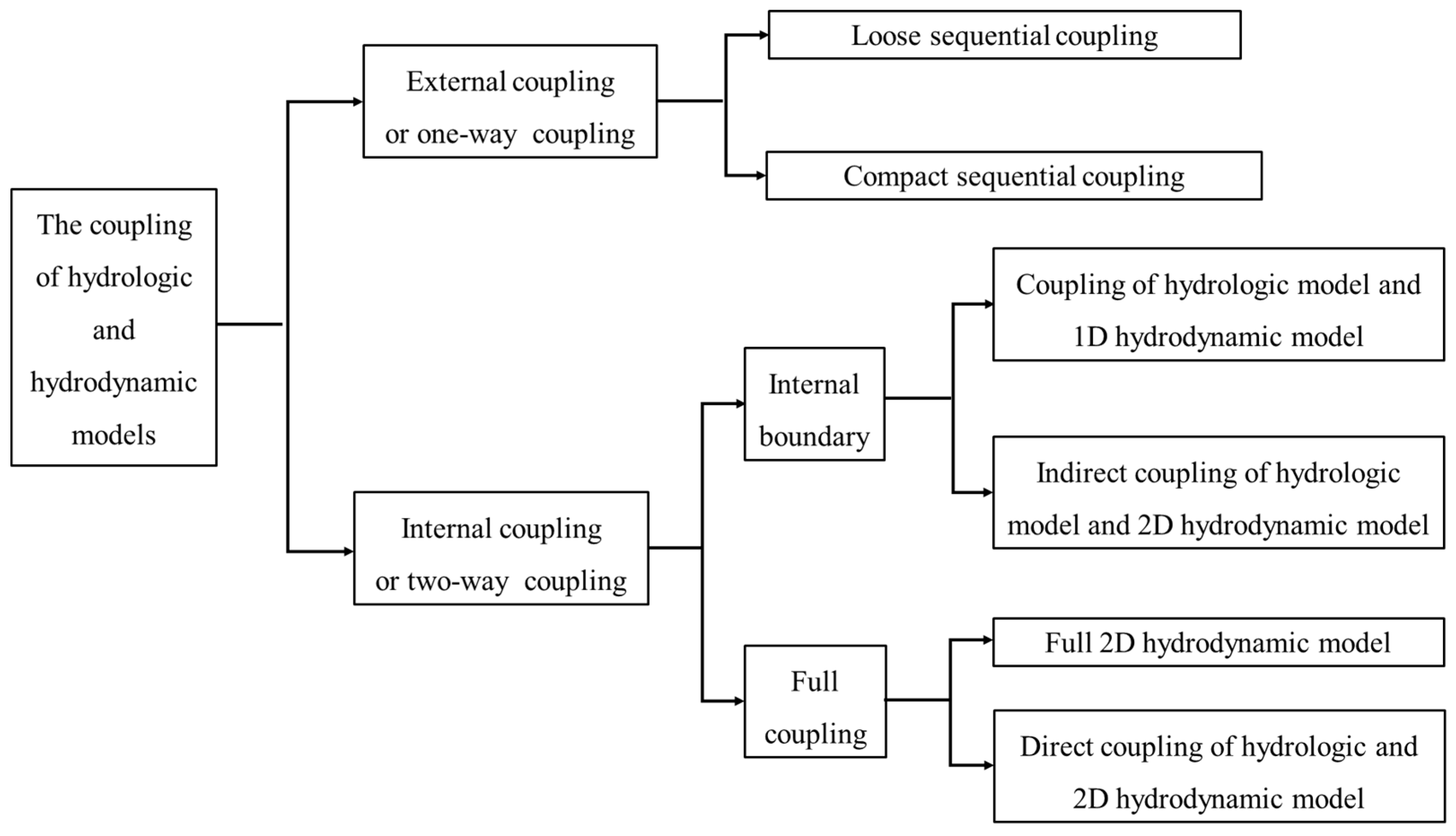
:1. Introduction
2. Methods
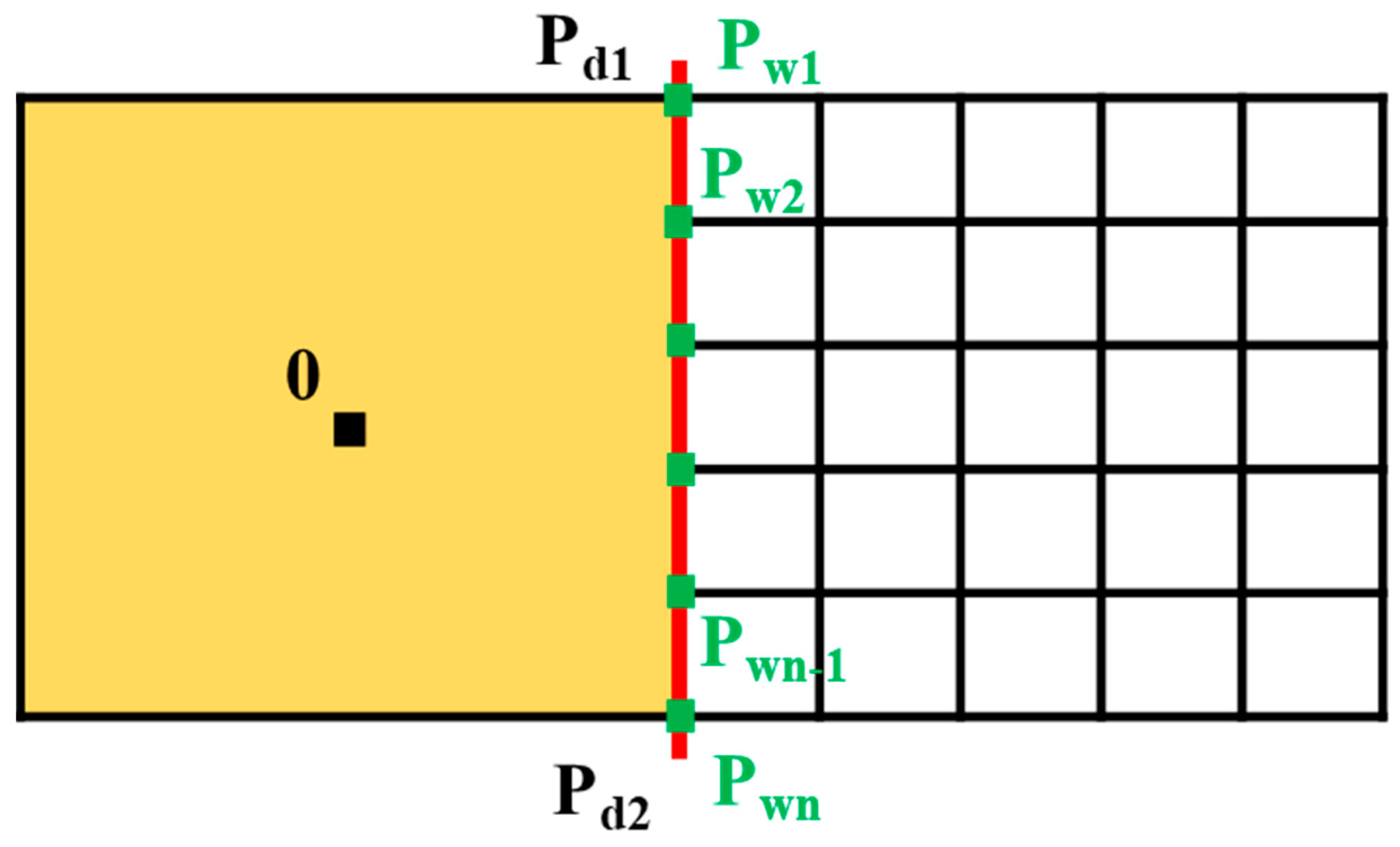
2.1. Zone Partition and Grid System
2.2. Description of the Coupled Surface Flow Routing Model
2.2.1. Runoff Generation
2.2.2. Surface Flow Routing
Shallow Water Equations
Diffusion Wave Equations
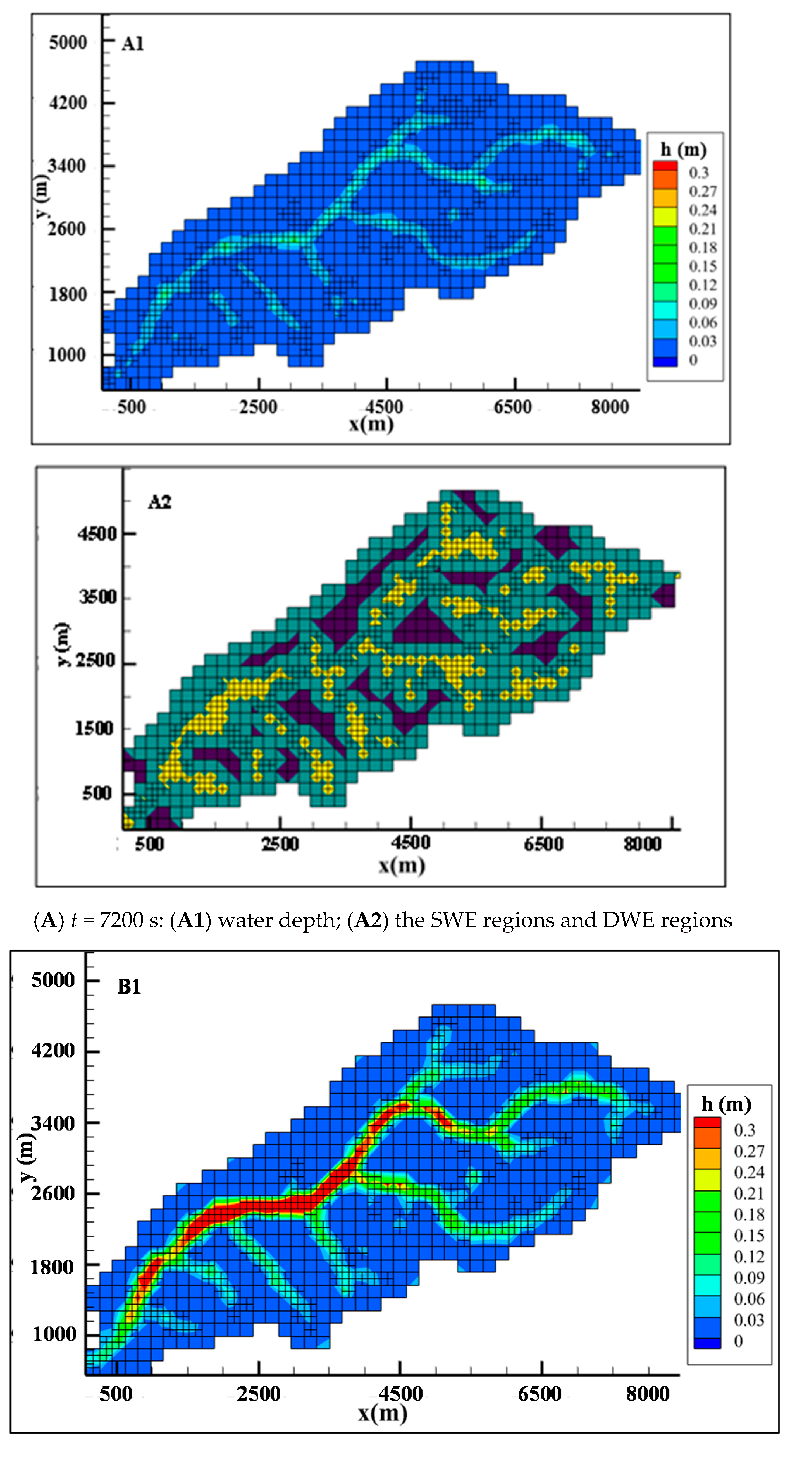
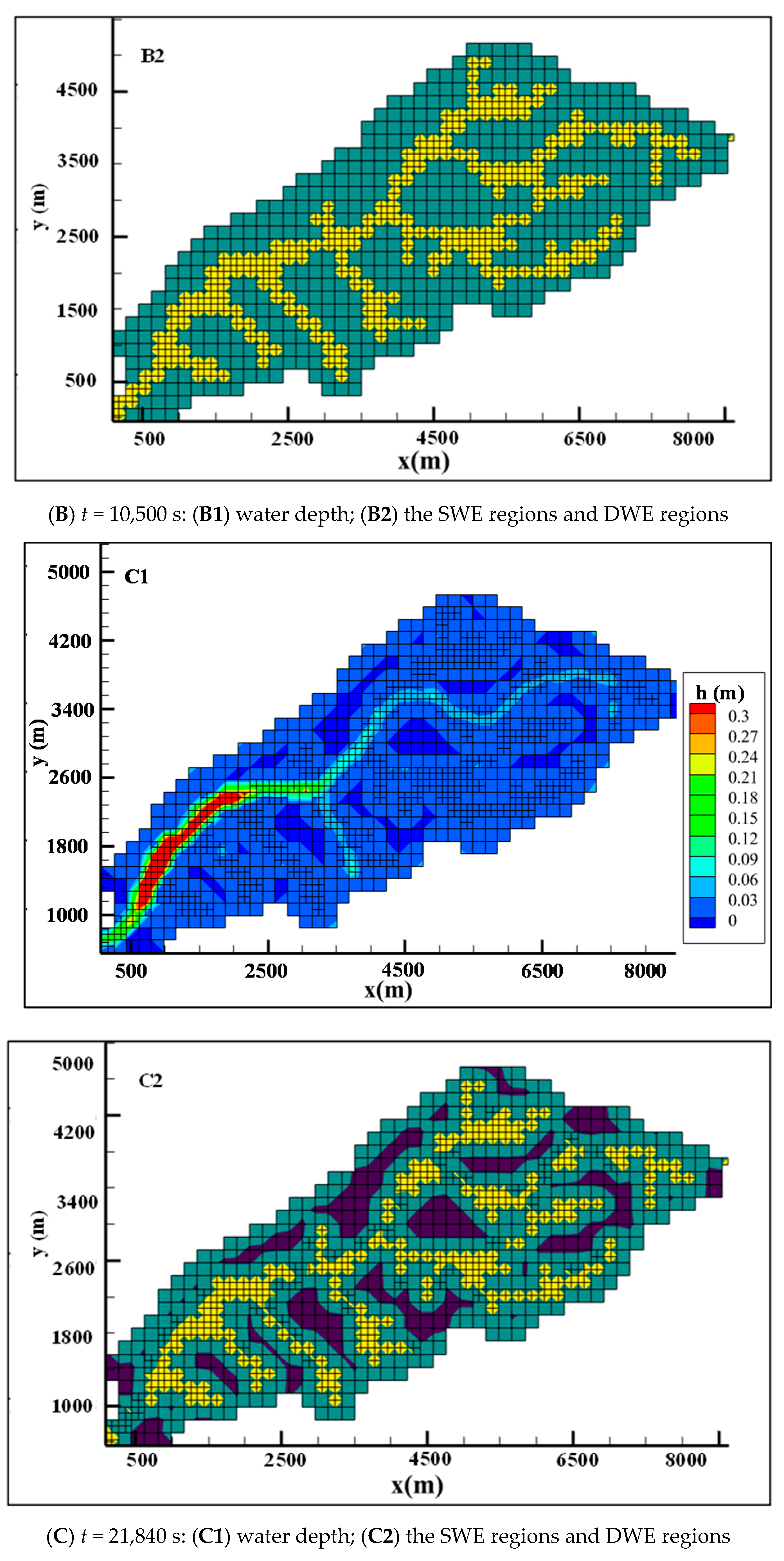
2.3. Coupling Strategies
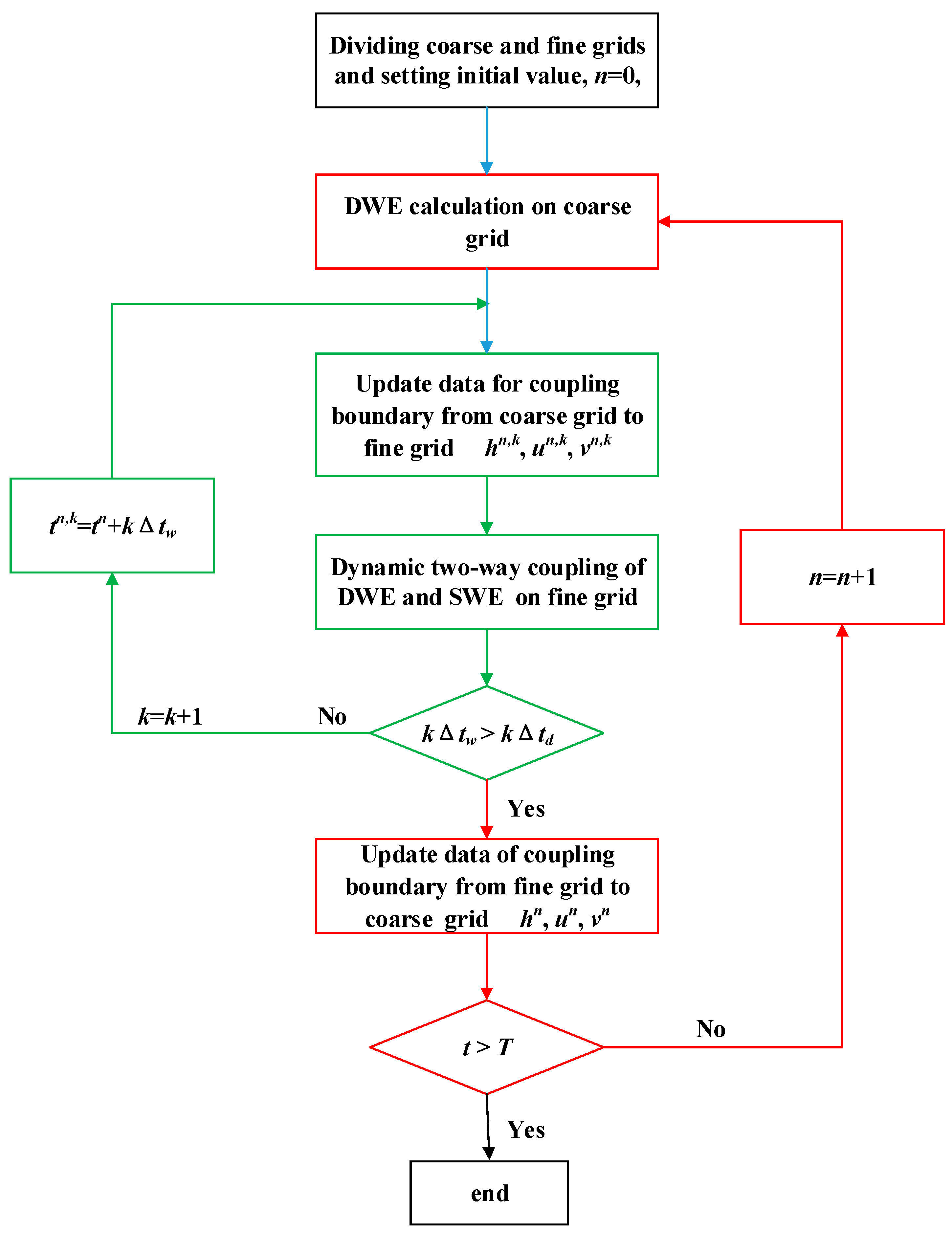
2.3.1. Multigrid and Variable Interpolation
- Step 1: The DWEs were used to simulate rainfall runoff on the coarse grid to obtain the water depth and flow velocity , .
- Step 2: The information, such as water depth and velocity, was updated from the coarse grid to fine grid. The water depth and flow velocity in shared nodes could be transmitted directly between different meshes, and linear interpolation was used to calculate the water depth and velocity in unshared nodes. Therefore, the water depth and velocity , on the coupling boundary between the coarse gird and fine grid were determined to drive the simulation on the fine grid.
- Step 3: The dynamic two-way coupling of the DWEs and SWEs was developed on the fine grid to obtain the water depth and velocity , .
- Steps 2 and 3 were repeated k times to obtain the data for the calculation of the DWEs at the next time on the coarse grid.
- Step 4: The water depth and velocity , were updated from the fine grid to coarse grid to drive the calculation of the DWEs on the coarse grid at n + 1 time.
- Steps 1–4 can be repeated many times and were not completed until time T.
2.3.2. Explicit Scheme and Numerical Stability
3. Applications
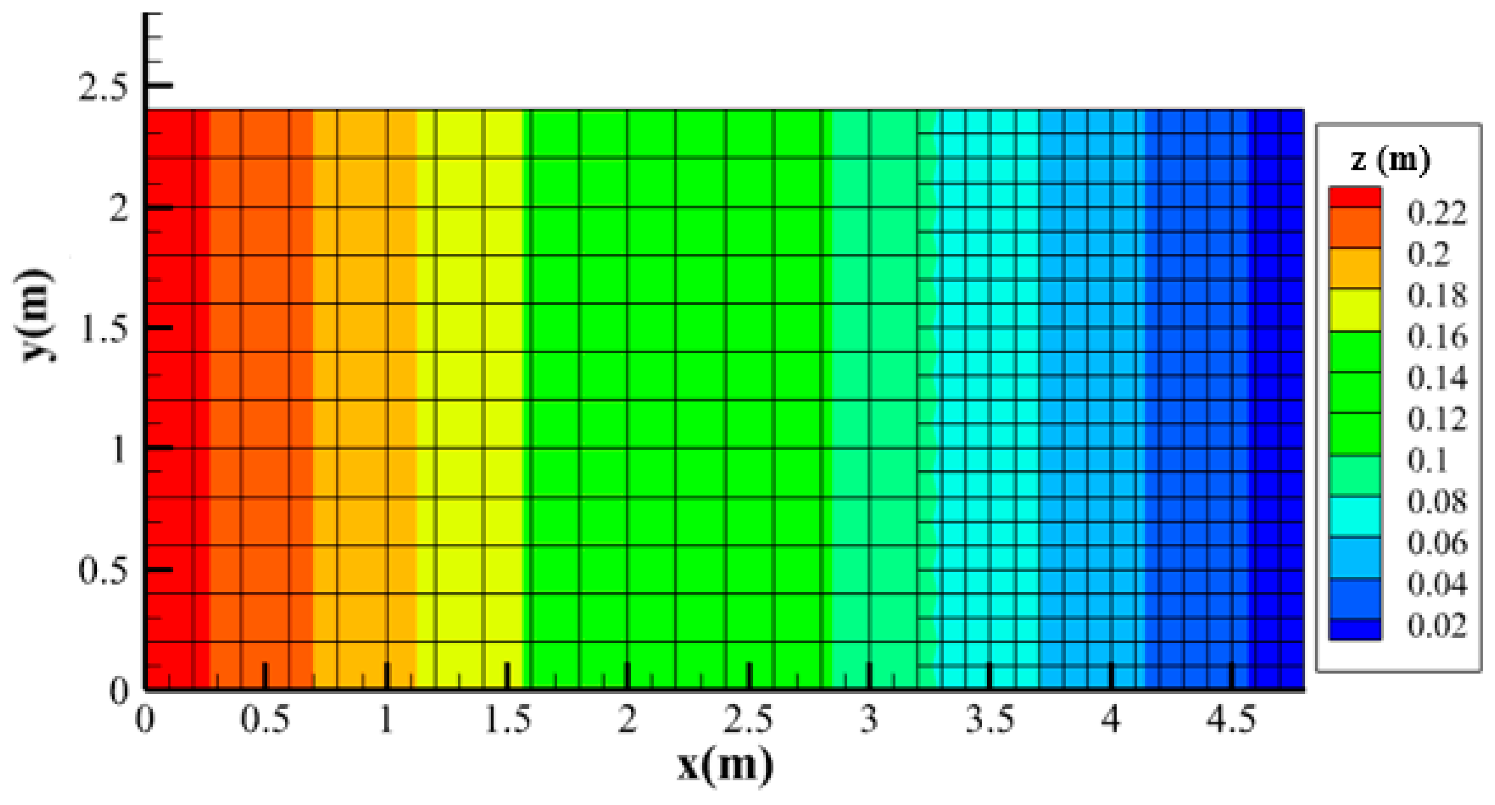
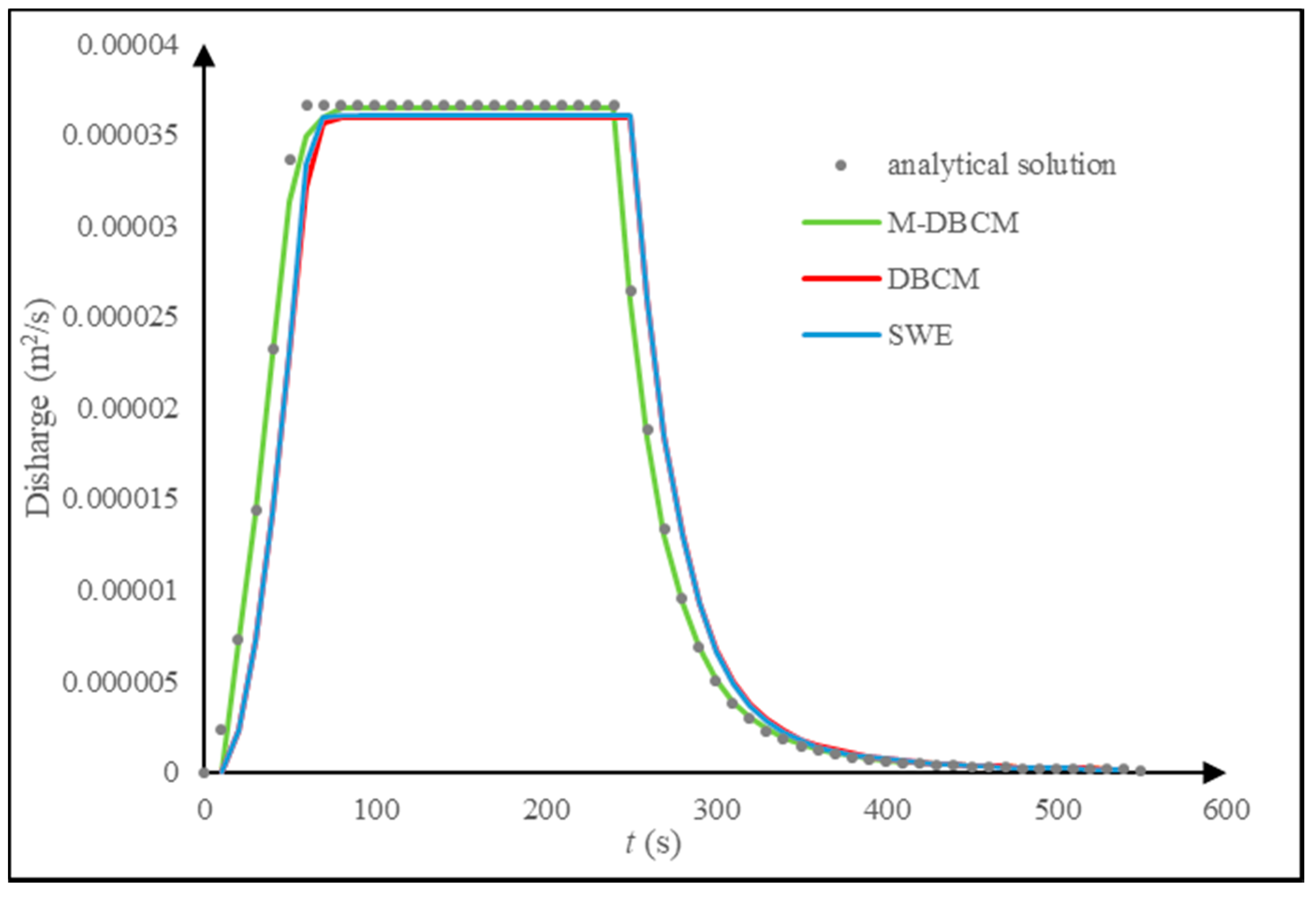
3.1. Rainfall Runoff over a Mild-Slope Plane
3.2. Rainfall Runoff over a Steep-Sloped Plane
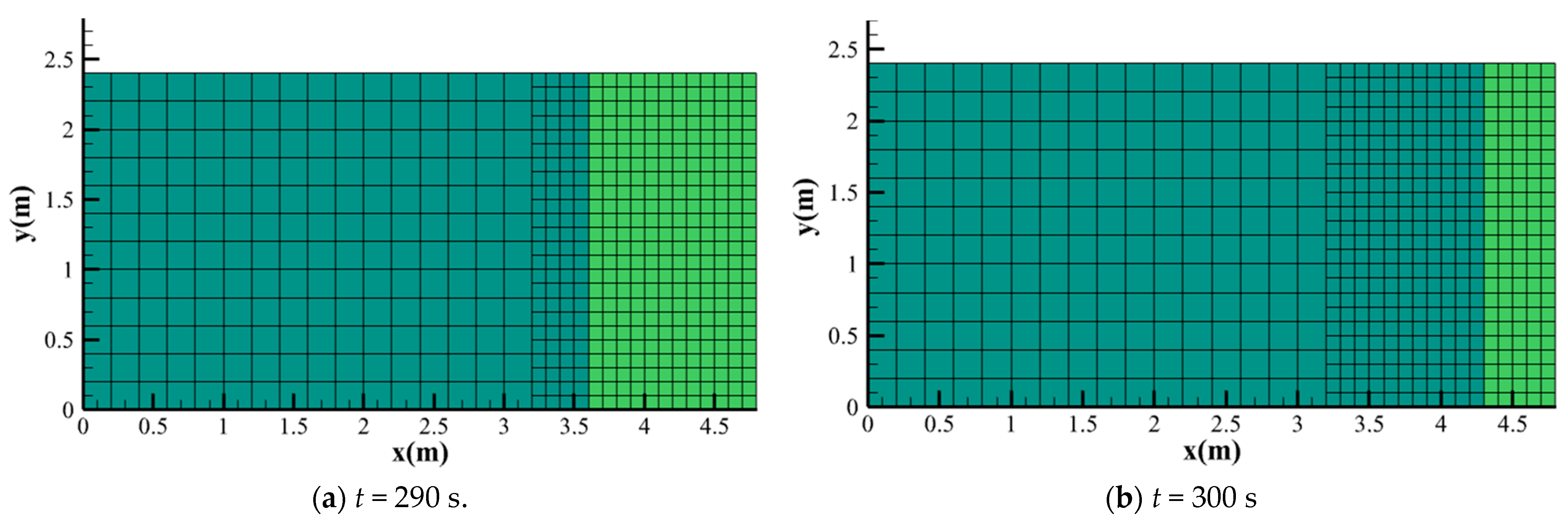
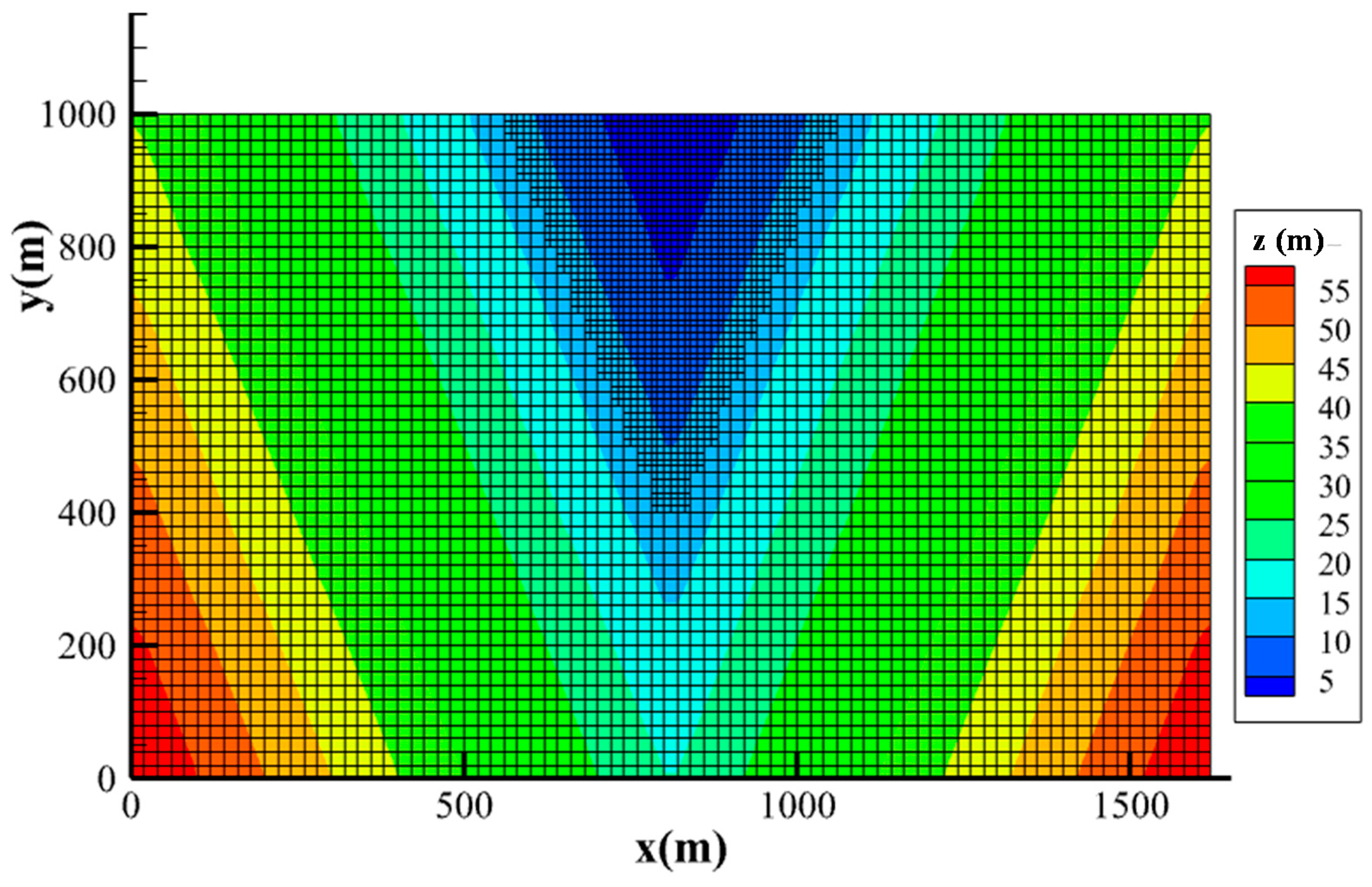
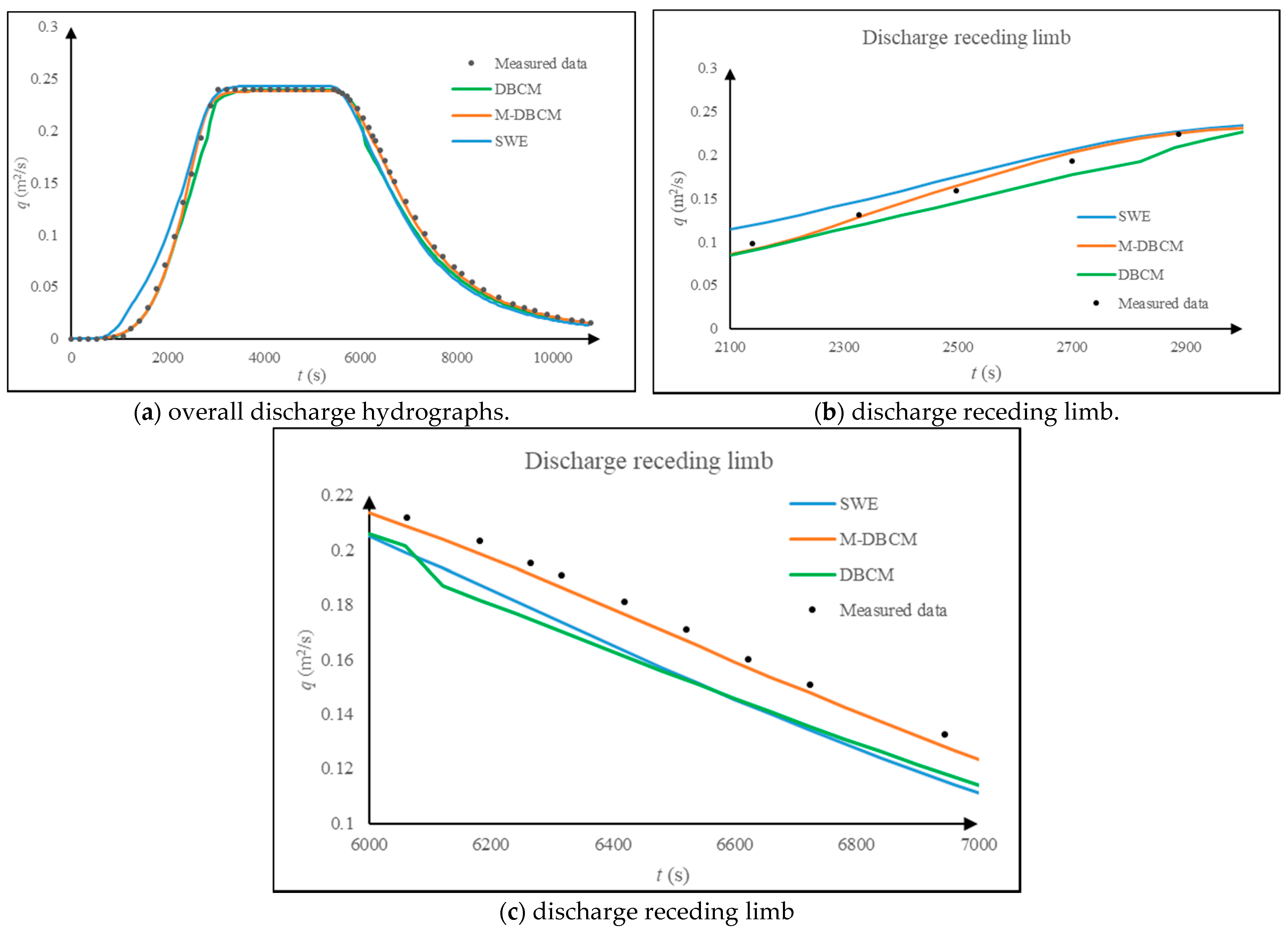
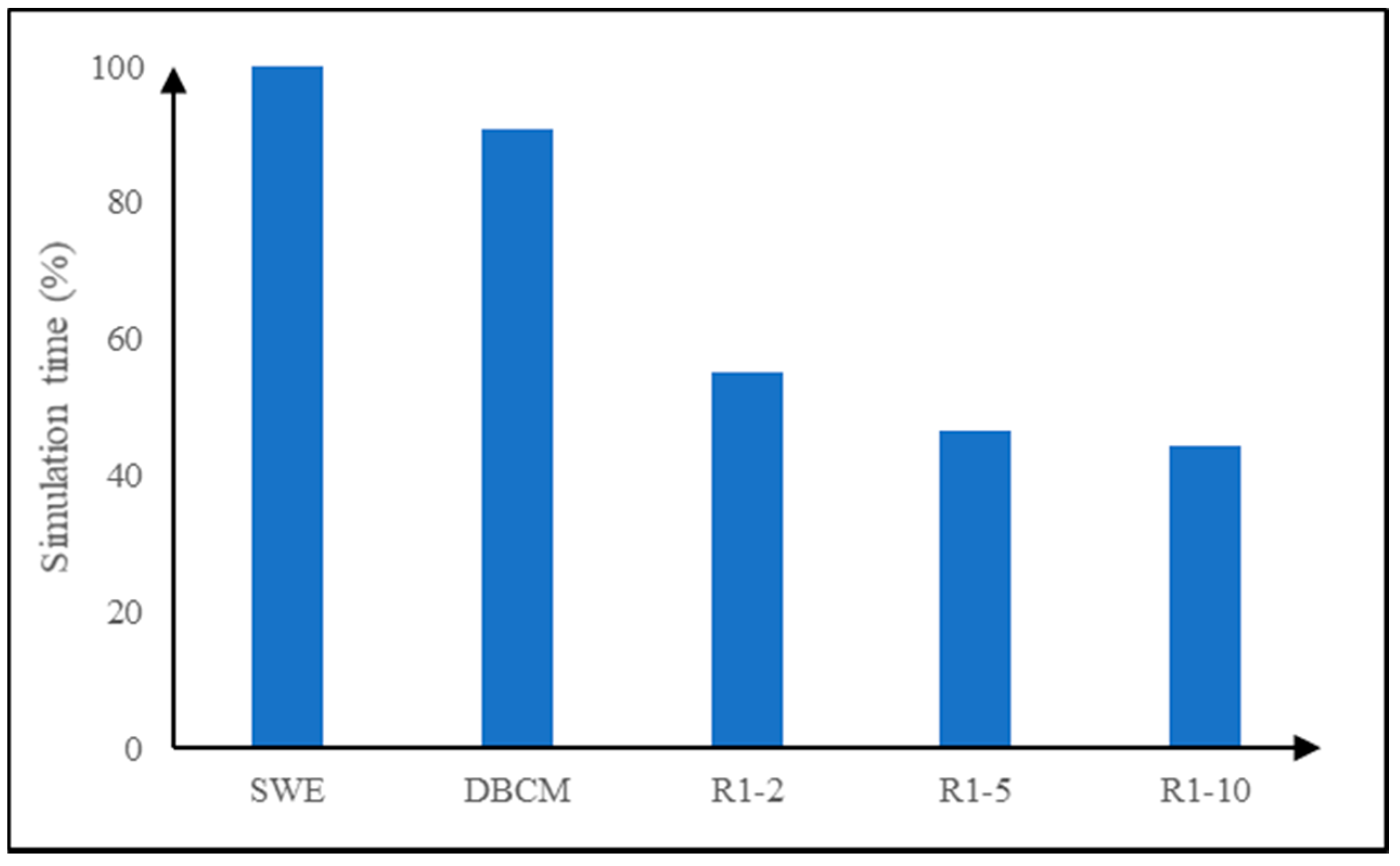
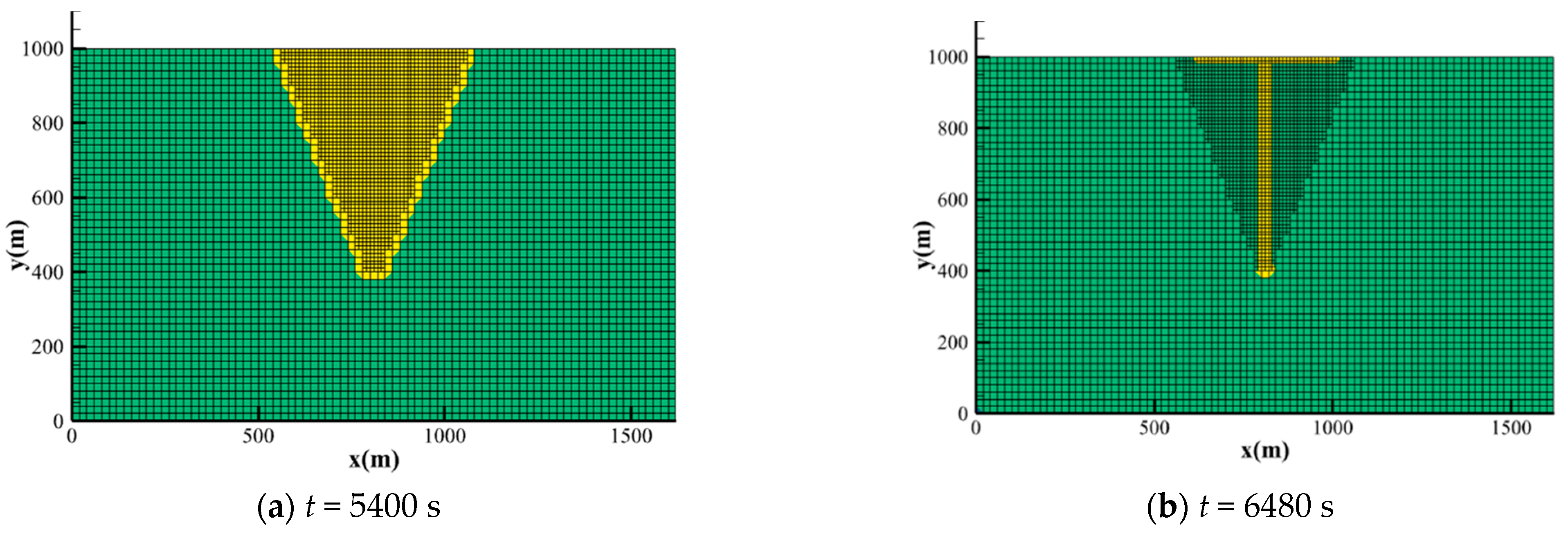
3.3. Rainfall Runoff over a V-Shaped Watershed
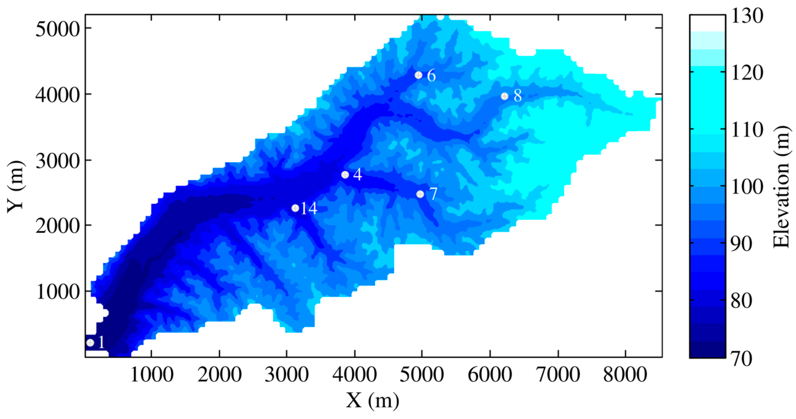
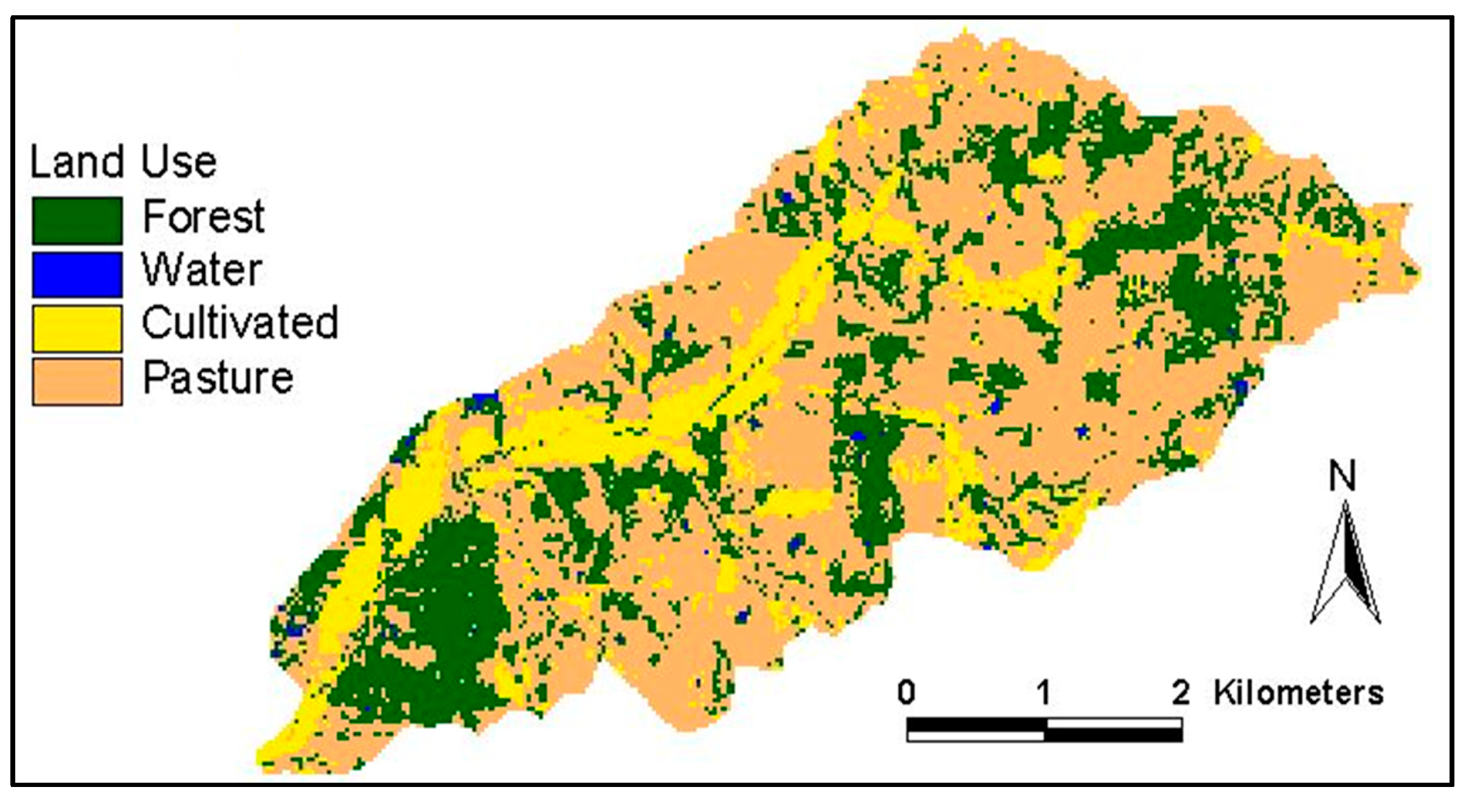
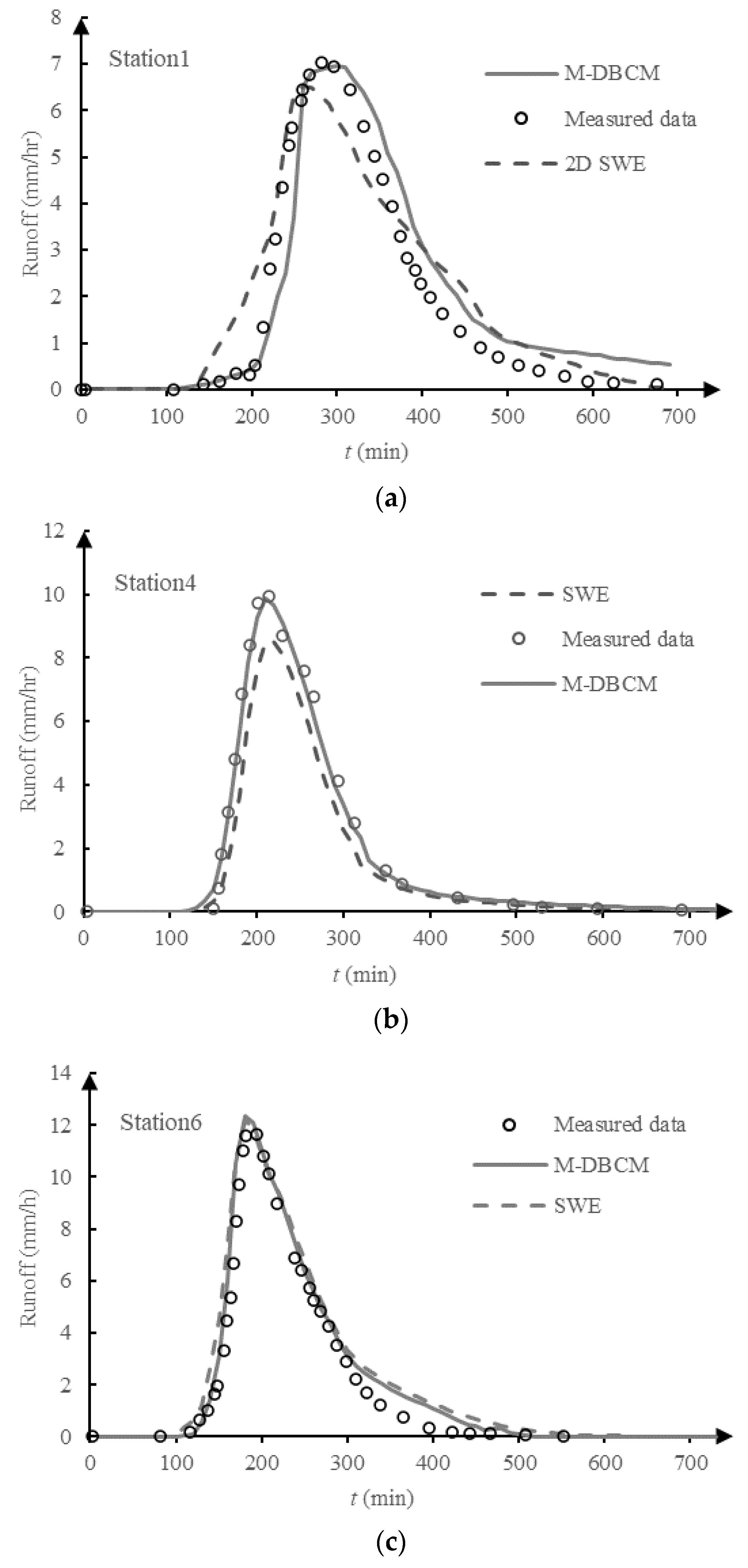
3.4. M-DBCM Implemented for a Natural Watershed
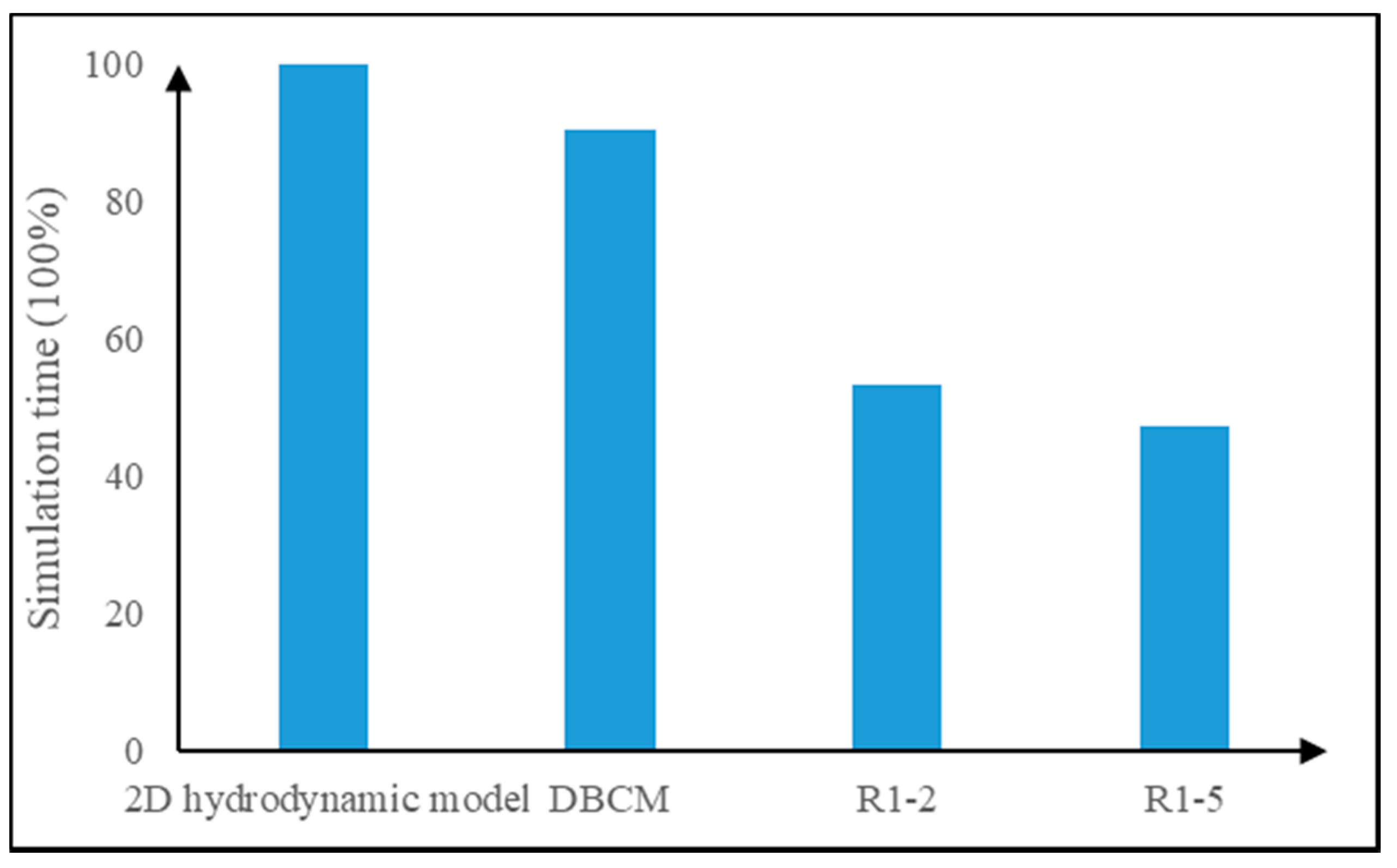
4. Discussion
5. Conclusions
Author Contributions
Funding
Institutional Review Board Statement
Informed Consent Statement
Data Availability Statement
Acknowledgments
Conflicts of Interest
References
- Tomasz, D.; Ewelina, S.; Joanna, W.D. Long-term impact of sediment deposition and erosion on water surface profiles in the Ner River. Water 2017, 9, 168–182. [Google Scholar]
- Hua, J.; Rui, L.; Yu, W.; Prasad, T. Flood-runoff in semi-arid and sub-humid regions, a case study: A simulation of Jianghe watershed in northern china. Water 2015, 7, 5155–5172. [Google Scholar]
- Leandro, J.; Chen, A.S.; Schumann, A. A 2D parallel diffusive wave model for floodplain inundation with variable time step (P-DWave). J. Hydrol. 2014, 517, 250–259. [Google Scholar] [CrossRef]
- Eum, H.-I.; Dibike, Y.; Prowse, T. Climate-induced alteration of hydrologic indicators in the athabasca river basin, alberta, canada. J. Hydrol. 2016, 544, 327–342. [Google Scholar] [CrossRef]
- Yang, W.; Long, D.; Bai, P. Impacts of future land cover and climate changes on runoff in the mostly afforested river basin in north china. J. Hydrol. 2019, 570, 201–219. [Google Scholar] [CrossRef]
- Yu, C.; Duan, J. Two-dimensional hydrodynamic model for surface-flow routing. J. Hydraul. Eng. 2014, 140, 04014045. [Google Scholar] [CrossRef]
- Mishra, B.K.; Emam, A.R.; Masago, Y.; Kumar, P.; Regmi, R.K.; Fukushi, K. Assessment of future flood inundations under climate and land use change scenarios in the ciliwung river basin, jakarta. J. Flood Risk Manag. 2018, 11, S1105–S1115. [Google Scholar] [CrossRef]
- Liu, Z.J.; Hashim, N.B.; Kingery, W.L.; Huddleston, D.H.; Xia, M. Hydrodynamic modeling of St. Louis Bay estuary and watershed using EFDC and HSPF. J. Coast. Res. 2008, 52, 107–116. [Google Scholar] [CrossRef]
- Li, W.; Lin, K.; Zhao, T.; Lan, T.; Chen, X.; Du, H.; Chen, H. Risk assessment and sensitivity analysis of flash floods in ungauged basins using coupled hydrologic and hydrodynamic models. J. Hydrol. 2019, 572, 108–120. [Google Scholar] [CrossRef]
- Dargahi, B.; Setegn, S.G. Combined 3D hydrodynamic and watershed modeling of Lake Tana, Ethiopia. J. Hydrol. 2011, 398, 44–64. [Google Scholar] [CrossRef]
- Bravo, J.M.; Allasia, D.; Paz, A.R.; Collischonn, W.; Tucci, C.E.M. Coupled Hydrologic-Hydraulic Modeling of the Upper Paraguay River Basin. J. Hydrol. Eng. 2012, 17, 635–646. [Google Scholar] [CrossRef]
- Laganier, O.; Ayral, P.A.; Salze, D.; Sauvagnargues, S. A coupling of hydrologic and hydraulic models appropriate for the fast floods of the gardon river basin (France). Nat. Hazards Earth Syst. Sci. 2014, 14, 2899–2920. [Google Scholar] [CrossRef] [Green Version]
- Hdeib, R.; Abdallah, C.; Colin, F.; Brocca, L.; Moussa, R. Constraining coupled hydrological-hydraulic flood model by past storm events and post-event measurements in data-sparse regions. J. Hydrol. 2018, 540, 160–176. [Google Scholar] [CrossRef]
- Choi, C.C.; Mantilla, R. Development and analysis of GIS tools for the automatic implementation of 1D hydraulic models coupled with distributed hydrological models. J. Hydrol. Eng. 2015, 20, 06015005. [Google Scholar] [CrossRef]
- Gomes, M.M.D.; Verçosa, L.F.D.; Cirilo, J.A. Hydrologic models coupled with 2D hydrodynamic model for high-resolution urban flood simulation. Nat. Hazards 2021, 108, 3121–3157. [Google Scholar] [CrossRef]
- Bhola, P.K.; Leandro, J.; Disse, M. Framework for offline flood inundation forecasts for two-dimensional hydrodynamic models. Geosciences 2018, 8, 346. [Google Scholar] [CrossRef] [Green Version]
- Liu, Z.; Zhang, H.; Liang, Q. A coupled hydrological and hydrodynamic model for flood simulation. Hydrol. Res. 2019, 50, 580–606. [Google Scholar] [CrossRef]
- Thompson, J.R.; Sørenson, H.R.; Gavin, H.; Refsgaard, A. Application of the coupled MIKE SHE/MIKE 11 modelling system to a lowland wet grassland in southeast England. J. Hydrol. 2004, 590, 151–179. [Google Scholar] [CrossRef]
- Chalkidis, I.; Seferlis, M.; Sakellariou-Makrantonaki, M. Evaluation of the environmental impact of an irrigation network in a ramsar area of the greek part of the strymonas river basin using a coupled Mike SHE/Mike 11 modelling system. Glob. Nest J. 2016, 18, 56–66. [Google Scholar]
- Laganier, O.; Ayral, P.A.; Salze, D.; Sauvagnargues, S. A coupling of hydrologic and hydraulic models appropriate for the fast floods of the Gardon river basin (France): Results and comparisons with others modelling options. Nat. Hazards Earth Syst. Sci. 2013, 1, 4635–4680. [Google Scholar] [CrossRef] [Green Version]
- Chen, W.; Huang, G.; Han, Z. Urban stormwater inundation simulation based on SWMM and diffusive overland-flow model. Water Sci. Technol. 2017, 76, 3392–3403. [Google Scholar] [CrossRef]
- Chen, W.; Huang, G.; Han, Z.; Wang, W. Urban inundation response to rainstorm patterns with a coupled hydrodynamic model: A case study in Haidian Island, China. J. Hydrol. 2018, 564, 1022–1035. [Google Scholar] [CrossRef]
- Seyoum, S.D.; Vojinovic, Z.; Price, R.K.; Weesakul, S. Coupled 1D and noninertia 2D flood inundation model for simulation of urban flooding. J. Hydraul. Eng. 2012, 138, 23–34. [Google Scholar] [CrossRef]
- Wu, J.; Yang, R.; Song, J. Effectiveness of low-impact development for urban inundation risk mitigation under different scenarios: A case study in Shenzhen, China. Nat. Hazards Earth Syst. Sci. 2018, 18, 2525–2536. [Google Scholar] [CrossRef] [Green Version]
- Brewer, S.K.; Worthington, T.A.; Mollenhauer, R.; Stewart, D.R.; Mcmanamay, R.A.; Guertault, L.; Moore, D. Synthesizing models useful for ecohydrology and ecohydraulic approaches: An emphasis on integrating models to address complex research questions. Ecohydrology 2018, 11, e1966. [Google Scholar] [CrossRef]
- Hou, J.; Liang, Q.; Simons, F.; Hinkelmann, R. A 2D well balanced shallow flow model for unstructured grids with novel slope source term treatment. Adv. Water Resour. 2013, 52, 107–131. [Google Scholar] [CrossRef]
- Yu, C.; Duan, J.G. Simulation of surface runoff using hydrodynamic model. J. Hydrol. Eng. 2017, 22, 04017006. [Google Scholar] [CrossRef]
- Kim, J.; Warnock, A.; Ivanov, V.Y.; Katopodes, N.D. Coupled modeling of hydrologic and hydrodynamic processes including overland and channel flow. Adv. Water Resour. 2012, 37, 104–126. [Google Scholar] [CrossRef]
- Jiang, C.; Zhou, Q.; Yu, W.; Yang, C.; Lin, B. A dynamic bidirectional coupled surface flow model for flood inundation simulation. Nat. Hazards Earth Syst. Sci. 2021, 21, 497–515. [Google Scholar] [CrossRef]
- Liang, Q. Flood simulation using a well-balanced shallow flow model. J. Hydraul. Eng. 2010, 136, 669–675. [Google Scholar] [CrossRef]
- Leer, B.V. Towards the ultimate conservative difference scheme V: A second order sequel to Godunov′s method. J. Comput. Phys. 1979, 32, 101–136. [Google Scholar] [CrossRef]
- Delis, A.; Nikolos, I. A novel multidimensional solution reconstruction and edge-based limiting procedure for unstructured cell-centered finite volumes with application to shallow water dynamics. Int. J. Numer. Methods Fluids 2013, 71, 584–633. [Google Scholar] [CrossRef]
- Panday, S.; Huyakorn, P.S. A fully coupled physically-based spatially-distributed model for evaluating surface/subsurface flow. Adv. Water Resour. 2004, 27, 361–382. [Google Scholar] [CrossRef]
- Lai, Y.G. Watershed runoff and erosion modeling with a hybrid mesh model. J. Hydrol. Eng. 2009, 14, 15–26. [Google Scholar] [CrossRef]
- Sánchez, R.R. GIS-Based Upland Erosion Modeling, Geovisualization and Grid Size Effects on Erosion Simulations with CASC2D-SED. Ph.D. Thesis, Colorado State University, Fort Collins, CO, USA, June 2002. [Google Scholar]
- Blackmarr, W. Documentation of Hydrologic, Geomorphic, and Sediment Transport Measurements on the Goodwin Creek Experimental Watershed, Northern Mississippi, for the Period 1982—1993; Technical Report for United States Department of Agriculture: Oxford, MS, USA, October 1995. [Google Scholar]


| Land Use | Forest | Water | Cultivated Land | Pasture |
|---|---|---|---|---|
| Manning’s roughness coefficient | 0.05 | 0.01 | 0.03 | 0.04 |
| Soil Type | Calloway | Fallaya | Grenada | Loring | Collins | Memphis | Cullied Land |
|---|---|---|---|---|---|---|---|
| Infiltration coefficients | 3.36 | 3.072 | 3.552 | 3.648 | 3.456 | 4.32 | 3.84 |
| Name | M-DBCM | SWE | CASC2D | Yu and Duan |
|---|---|---|---|---|
| Station 1 | 0.93 | 0.97 | 0.62 | 0.96 |
| Station 4 | 0.56 | 0.42 | 0.84 | 0.73 |
| Station 6 | 0.37 | 0.30 | 1.03 | 1.06 |
| Station 7 | 1.05 | 1.53 | 1.42 | 1.18 |
| Station 8 | 0.89 | 0.97 | 1.88 | 1.04 |
| Station 14 | 1.23 | 1.31 | 1.53 | 1.07 |
Publisher’s Note: MDPI stays neutral with regard to jurisdictional claims in published maps and institutional affiliations. |
© 2021 by the authors. Licensee MDPI, Basel, Switzerland. This article is an open access article distributed under the terms and conditions of the Creative Commons Attribution (CC BY) license (https://creativecommons.org/licenses/by/4.0/).
Share and Cite
Shen, Y.; Jiang, C.; Zhou, Q.; Zhu, D.; Zhang, D. A Multigrid Dynamic Bidirectional Coupled Surface Flow Routing Model for Flood Simulation. Water 2021, 13, 3454. https://doi.org/10.3390/w13233454
Shen Y, Jiang C, Zhou Q, Zhu D, Zhang D. A Multigrid Dynamic Bidirectional Coupled Surface Flow Routing Model for Flood Simulation. Water. 2021; 13(23):3454. https://doi.org/10.3390/w13233454
Chicago/Turabian StyleShen, Yanxia, Chunbo Jiang, Qi Zhou, Dejun Zhu, and Di Zhang. 2021. "A Multigrid Dynamic Bidirectional Coupled Surface Flow Routing Model for Flood Simulation" Water 13, no. 23: 3454. https://doi.org/10.3390/w13233454