Article

A Polynomial Method Approximating S-Curve with Limited Availability of Reliable Rainfall Data

by
Kee-Won Seong
1 and
Jang Hyun Sung
2,*
1
Department of Civil and Environmental Engineering, Konkuk University, 120 Neungdong-ro, Gwangjin-gu, Seoul 05029, Korea
2
Han River Flood Control Office, Ministry of Environment, 328 Dongjak-daero, Seocho-gu, Seoul 06501, Korea
*
Author to whom correspondence should be addressed.
Water 2021, 13(23), 3447; https://doi.org/10.3390/w13233447
Submission received: 7 October 2021 / Revised: 18 November 2021 / Accepted: 1 December 2021 / Published: 4 December 2021
(This article belongs to the Section Hydrology)

Abstract

:
A methodology named the step response separation (SRS) method for deriving S-curves solely from the data for basin runoff and the associated instantaneous unit hydrograph (IUH) is presented. The SRS method extends the root selection (RS) method to generate a clearly separated S-curve from runoff incorporated in mathematical procedure utilizing the step response function. Significant improvements in performance are observed in separating the S-curve with rainfall. A procedure to evaluate the hydrologic stability provides ways to minimize the oscillation of the S-curve associated with the determination of infiltration and baseflow. The applicability of the SRS method to runoff reproduction is examined by comparison with observed basin runoff based on the RS method. The SRS method applied to storm events for the Nenagh basin resulted in acceptable S-curves and showed its general applicability to optimization for rainfall-runoff modeling.

1. Introduction

This paper is the sequel of a previously suggested methodology for smoothing the oscillatory S-curve [1], in which a model was presented for determining the oscillation-reduced S-curve and associated instantaneous unit hydrograph (IUH) model using the Savitzky-Golay smoothing and differentiation filter.
The concept of the S-curve has been widely applied in rainfall–runoff analysis since its introduction in the unit hydrograph (UH) method [2,3]. The S-curve represents a direct runoff due to the effective rainfall applied over an infinite time, and its intensity is one-unit depth per unit of time. The role of the S-curve is to alter a UH of arbitrary duration into a UH of desired duration. The conventional method to generate an S-curve requires surface runoff data and corresponding effective rainfall. However, estimating accurately the effective rainfall for S-curve generation is difficult mainly because of problems related to the estimation of a real rainfall and to the determination of the reduction in total rainfall due to infiltration, which is affected by the uncertain soil moisture condition of basins and groundwater behavior [4,5]. Mathematically, these difficulties result in a hydrologically unstable system. Following, a problem arises in determining the S-curve of a linear rainfall-runoff system, since an oscillatory function is likely to be obtained. This problem can be circumvented by developing a method deriving an S-curve without using rainfall data.
The main objectives of this study are to estimate an S-curve without observed rainfall data and to investigate the hydrologic stability of rainfall-runoff data by using the derived S-curve. The approach adopted in this study relies on the root selection (RS) method [6]. This study names the suggested procedure as the step response separation (SRS) method. The RS method only requires runoff data from a single storm of the basin of interest to give a UH estimate [3]. In the RS method, the UH is determined based on the shape traced by the complex roots of the runoff polynomial on an Argand diagram, which yields some considerable applications. For example, the method was adopted in developing a design hydrograph in an arid basin [7], in identifying the quick and the slow components of runoff [4], and in synthesizing the Clark IUH [8]. However, very little research has been conducted on the RS method despite its advantages, mainly because of practical reasons since very high-order polynomials reflecting direct runoffs should be manipulated to derive UH ordinates [9]. Another reason is that the method of using an Argand diagram is subjective and cumbersome. Therefore, even when there is direct runoff data, synthetic UHs are often used in practice. However, in this process, important information about watersheds and rainfall-runoff may be lost. This important information includes the runoff characteristics and hydrological stability of the basin. Therefore, deriving UH through polynomial analysis is hydrologically meaningful.
In the present study, this paper develops the procedure for estimating an S-curve solely from basin runoff data by improving the defects of the existing method and examines the hydrologic stability of the resulting rainfall-runoff system. To that goal, this study uses cumulative runoff in the RS method. The applicability of the proposed methodology is evaluated using rainfall-runoff data for the Nenagh River at Clarianna, Ireland [10,11]. The performance of the derived S-curve and corresponding IUH is evaluated by the standard errors and Nash-Sutcliffe criterion. The proposed method is found to be more objective and distinct to generate hydrologic responses and be capable of checking the hydrologic stability of rainfall-runoff system.

2. The Proposed Method

2.1. Procedure of the Proposed Method

The impulse response function of a linear system indicates the system response to an instantaneous impulse of unit volume of input applied at time t = 0 . In hydrology, it is assumed that basins behave as linear system, and the impulse response function represents an IUH for the system-theoretical modeling of rainfall-runoff processes. Denoting the direct runoff by q ( t ) , the effective rainfall by x ( t ) , and the IUH by h ( t ) for stationary and casual systems, q ( t ) can be decomposed into IUH through the convolution integral:
q ( t ) = h ( t ) x ( t ) .
The unit step response function defines the response to a constant unit input for an infinite time. In hydrology, the unit step response function corresponds to the S-curve caused by a continuous effective rainfall of unit intensity. Thus, the S-curve can be obtained by substituting x ( t ) = μ ( t ) in Equation (1), which leads to:
s ( t ) = h ( t ) μ ( t )
where s ( t ) is an S-curve, and μ ( t ) is the unit step function defined as follows:
μ ( t ) = {   0 ,   t 0 1 ,   t > 0 .
In Equation (2), s ( t ) is the response to effective rainfall applied over an infinite time, and its intensity is one-unit depth per unit of time (e.g., 1 cm/h), which is equivalent to the unit step response defined as the output of a system due to the unit step function μ ( t ) .
This study suggests a convolution approach determining s ( t ) without using rainfall data. For this purpose, μ ( t ) is applied in Equation (1), which leads to
r ( t ) = q ( t ) μ ( t ) = [   h ( t ) x ( t )   ] μ ( t )
where r ( t ) denotes a cumulative function of the runoff (CFR). Using the properties of convolution (commutative law or associative law), Equation (4) is rearranged as:
r ( t ) = [ h ( t ) μ ( t ) ] x ( t ) = s ( t ) x ( t ) .
Thus, the S-curve s ( t ) can be determined by solving an inverse problem if r ( t ) is given.
When the effective rainfall x ( t ) is given as a hyetograph, the corresponding CFR can be represented as the discrete convolution of the rainfall hyetograph and S-curve. In the transformation technique for discrete time function, the Z-transform [12] is preferably used. Based on the Z-transformation theory, Equation (5) can be expressed in term of polynomials in z 1 ,
R ( z 1 ) = S ( z 1 )   X ( z 1 )
where R ( z 1 ) , S ( z 1 ) , and X ( z 1 ) are the Z-transforms of r ( t ) , s ( t ) , and x ( t ) , respectively.
When CFR data { r ( i T ) ,   i = 0 P } are collected repeatedly at fixed time interval T, R ( z 1 ) in Equation (6) can be formulated as:
R ( z 1 ) = i = 0 P r ( i T ) z i
where r ( i T ) z 1 represents the Z-transform of r ( i T ) calculated at t = i T . Equation (7) is a P-order polynomial in z 1 , which implies the existence of P roots. These roots consist of pairs of conjugate complex numbers so that they can be represented on a plane called the Argand diagram [12]. As with the existing RS method, the method of this study also ensures that the roots of Equation (7) depict a circular pattern on the Argand diagram with some points showing abnormal feature. The roots of the S-curve polynomial S ( z 1 ) , or the step response function, are selected based on the circle pattern, while the roots of the rainfall polynomial X ( z 1 ) are regarded as remaining roots. Using similar notation, S ( z 1 ) and X ( z 1 ) can be represented by the polynomials shown in Equations (8) and (9):
S ( z 1 ) = i = 0 N s ( i T ) z i
where N is the number of roots of the S-curve polynomial,
X ( z 1 ) = i = 0 M x ( i T ) z i
where M is the number of remaining roots. According to the linear convolution theory, the following relationship between the polynomials is satisfied:
P = M + N .
This study names the above-mentioned procedure as the SRS method.

2.2. Derivation of CFR Polynomial

To obtain the CFR polynomial R ( z 1 ) of Equation (7), the runoff polynomial Q ( z 1 ) , that is the Z-transform of q ( t ) , is also calculated according to Equation (4). When runoff data { q ( i T ) ,   i = 0 P } are collected repeatedly at fixed time interval T, Q ( z 1 ) can be formulated as:
Q ( z 1 ) = i = 0 P q ( i T ) z i
where q ( i T ) z 1 represents the Z-transform of q ( i T ) sampled at t = i T . The Z-transform of the unit step function μ ( t ) is defined as follows [13]:
Z ( μ ( t ) ) = U ( z 1 ) = 1 1 z 1 .
Thus, Equation (4) with respect to CFR becomes:
R ( z 1 ) = ( 1 1 z 1 )   Q ( z 1 ) = S ^ ( z 1 )   X ( z 1 )
where S ^ ( z 1 ) is an estimate of S ( z 1 ) . However, when using Equation (13), one may face the problem of factoring the polynomial. As already mentioned, S ( z 1 ) indicates the S-curve hydrograph, which implies that S ^ ( z 1 ) should be a real number coefficient polynomial in z 1 . To satisfy this condition, ( 1 z 1 ) should be a factor of the polynomial Q ( z 1 ) . However, in general, it is not the case, because the polynomial division of Equation (13) yields a remainder. So, this research uses a power expansion technique to approximate the rational function R ( z 1 ) . In fact, this expansion technique is mathematically plain because the divisor ( 1 z 1 ) constructs R ( z 1 ) by adding together the coefficients of Q ( z 1 ) lagged by one time step. Hence, the following equation for CFR can be formulated:
R ( z 1 ) = i = 1 P q ( i T ) z 1 1 z 1 = i = 1 P q ( i T ) ( j = i z j ) .
Therefore, Equation (14) can replace Equation (7). Solving for R ( z 1 ) = 0 , Equation (14) yields P roots. These P roots are drawn on the Argand diagram, and the pattern of these roots is investigated.

2.3. Inverse Transformation of S-Curve into Time Domain

As previously explained, similar to the RS method, the method of this study determines the S-curve polynomial S ( z 1 ) by selecting the complex roots based on the a priori expectation that the roots will draw a circle in the Argand diagram. The P roots obtained by solving Equation (14) are drawn on the Argand diagram. Among them, N roots pertain to the S-curves polynomial S ^ ( z 1 ) and M roots pertain to X ( z 1 ) . Hence, the S-curve can be written in the form of the polynomial:
S ( z 1 ) = s 1 z 1 +     + s N 1 z ( N 1 ) + s N z N
where the coefficients s 1 ,   s 2 ,     , and s N represent the ordinates of the S-curve. Note that these coefficients are not the exact values but the relative magnitude of each coordinate of the S-curve. Therefore, these values should be adjusted using the equilibrium of the S-curve. Based on S-curve theory, the coefficient s N of the highest term of Equation (15) should attain the equilibrium discharge q e q occurring at the base time of UH, and the value is determined from:
q e q = 0.2778 A d T [ m 3 s ]
where A is the watershed area (km2); d is the unit rainfall depth (1 cm); and, T is the sampling interval. Adjusted with q e q by a linear programming technique, the ordinates of the S-curve can be defined as follows:
s T = [ s T [ 1 ] , s T [ 2 ] , , s T [ N ] ] Τ
where s T [ 1 ] , s T [ 2 ] , , and s T [ N ] are the ordinates of the S-curve, s ( t ) . At t i = i T , s ( t ) can be represented by the ordinate of s T [ i ] . The S-curve s T can be transformed into UH of desired duration or into IUH h T = [ h 1 , h 2 , , h N ] Τ by a numerical differentiation method, for example, the digital filtering technique [1].

2.4. Model Performance Indices

Two different criteria are considered for evaluating the model performance of the SRS method. To do this, this study uses the derived IUHs for all storms by means of numerical differentiation of S-curves and their reproduced runoff.
As a model performance criterion, the standard errors (STDER) [14] are evaluated. STDER is defined by the following equation:
S T D E R = n = 1 N ( h n h r e f , n ) 2 w n N
where h n is the IUH ordinate at the nth time interval; h r e f , n is the ordinate of the referenced IUH at the same time; and w n is the weight given by:
w i = h r e f , i + h a v g 2 h a v g
where h a v g is the average value of the referenced IUH ordinates. A low value of STDER implies a good model, and the zero value of STDER means that the computed IUH perfectly matches with the referenced IUH. In addition, the performance of the SRS method is evaluated by the Nash–Sutcliffe criterion based on the reproduced runoff [15] given in Equation (20).
E = ( 1 j = 1 J ( q j q ^ j ) 2 j = 1 J ( q j q ¯ ) 2 ) × 100
where E is the Nash-Sutcliffe model efficiency coefficient: J is the number of observations; q j is the observed runoff at time j; q ^ j is the predicted runoff at time j determined from the proposed IUH; and q ¯ is the mean of the observed runoff. The closer E is to 100, the better the performance of the model [16]. The peak relative error, QB, is the difference in magnitude between the observed and estimated peaks and is used for model performance analysis [17].
Q B = q p q ^ p q p
where q p is the peak value of observed runoff; and q ^ p is the peak of estimated runoff. The closer QB is to 0, the better the performance of the model.

3. Results

The proposed methodology using CFR and the Argand diagram is applied to the estimation of the S-curve S ^ ( z 1 ) . The considered basin is the Nenagh River at Clarianna, Ireland, with an area of 295 km2 [6]. The catchment of Clarianna has four rain gauges reading daily records and one recording continuously. The present study refers to the data for five of 22 storms on the Nenagh River basin, which were examined by using the least squares analysis [10]. The considered five storm events present strong difficulty in identifying the roots of CFR and are referred to as events 5, 13, 14, 15, and 20. Note that storm event 13 will be used for identifying the sensitivity of the proposed method. For the selected events, the peaks of the direct runoffs recorded a range from 13.19 to 23.52 m3s−1 when the measurements are made at 3 h ( = T ) interval. The equilibrium discharge q e q is 273 m3s−1. The major features of the selected storm events are listed in Table 1.
The proposed method determines the S-curve S ( z 1 ) by selecting the complex roots based on the a priori expectation that the roots will describe a circle in the Argand diagram for the roots of the CFR polynomial. The Argand diagrams of storm events 5, 14, 15, and 20 are plotted in Figure 1.
The root separation procedure by the SRS method developed by modifying the existing RS method [6] is as follows: (1) select the S-curve roots based on the circle pattern; (2) construct the S-curve using the so-separated roots; and (3) combine the remaining roots to form an estimate of effective rainfall. The complex roots for the direct runoff polynomial for each event plotted in Figure 1 are relevant to the S-curve S ^ ( z 1 ) and rainfall X ( z 1 ) . In Figure 1, the roots of S ^ ( z 1 ) represented by dots are spread at a practically equal angle from each other and describe almost perfect circles with a slightly increasing radius from left to right. Approximating the polynomial for S ( z 1 ) is achieved by combining the roots on these circles. To check the validity of the approximation, S ^ ( z 1 ) is illustrated in Figure 2.
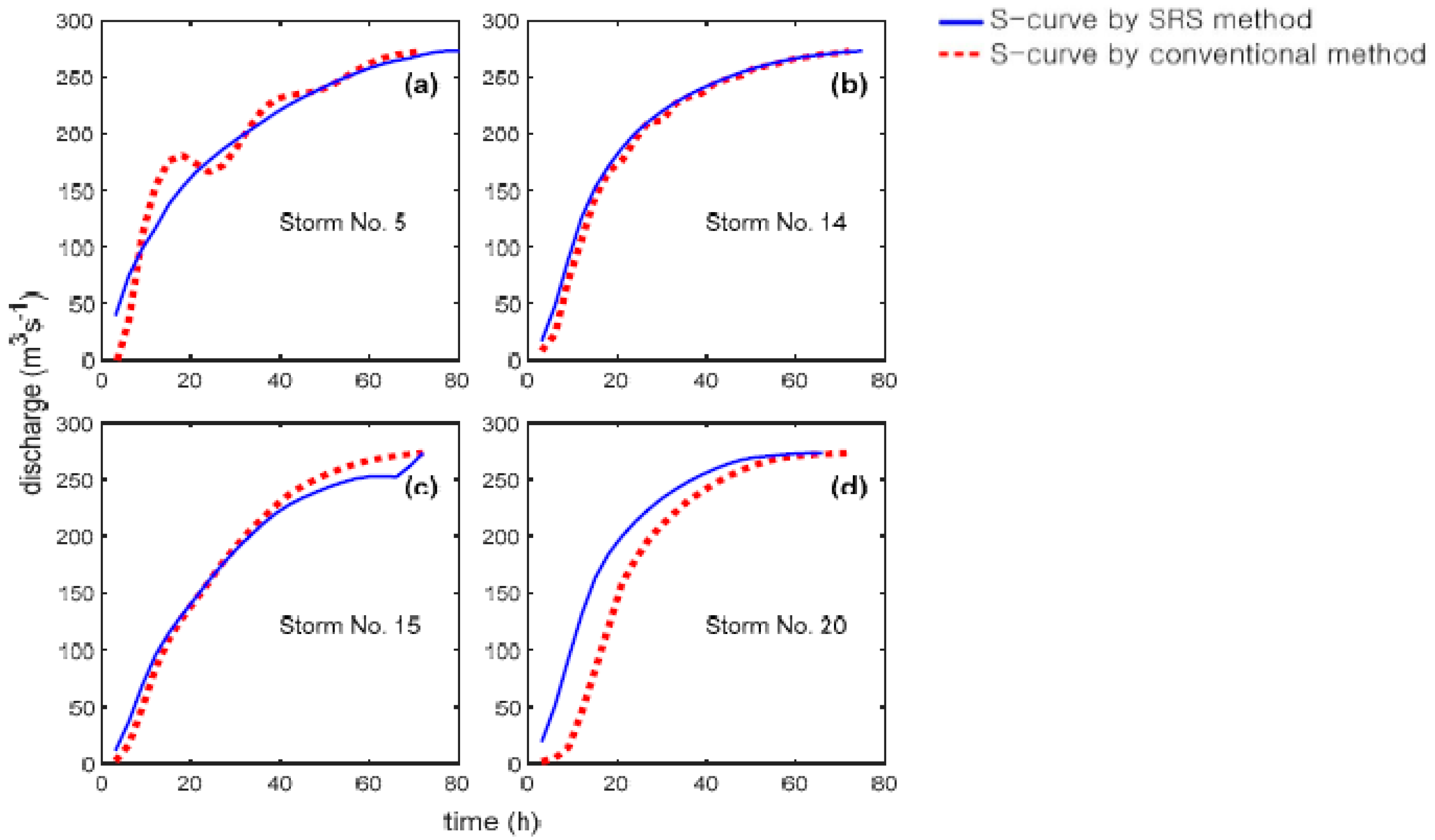
In Figure 2, the estimated S-curves for the four storms were derived by the SRS method and are compared with those obtained by the conventional method in which the 3 h S-curves are computed by successively adding the coordinates of 3 h UHs lagged by the duration (=3 h) until 24 time steps. The 3 h UH of each storm is calculated by means of the least square method. From the figure, it is seen that the SRS method generates smooth S-curves when using the roots of S ^ ( z 1 ) represented in the Argand diagram in Figure 1. Moreover, the coordinates of S-curves using the SRS method agree well with those of the conventional method in all storms except for storm event 20. From the comparison of the coefficients of the S ^ ( z 1 ) polynomial with the other S-curves, this study can infer that a nonlinear dynamic system of rainfall–runoff structure to obtain accurate surface runoff coordinates and relevant rainfall values gave rise to this inconsistent behavior.
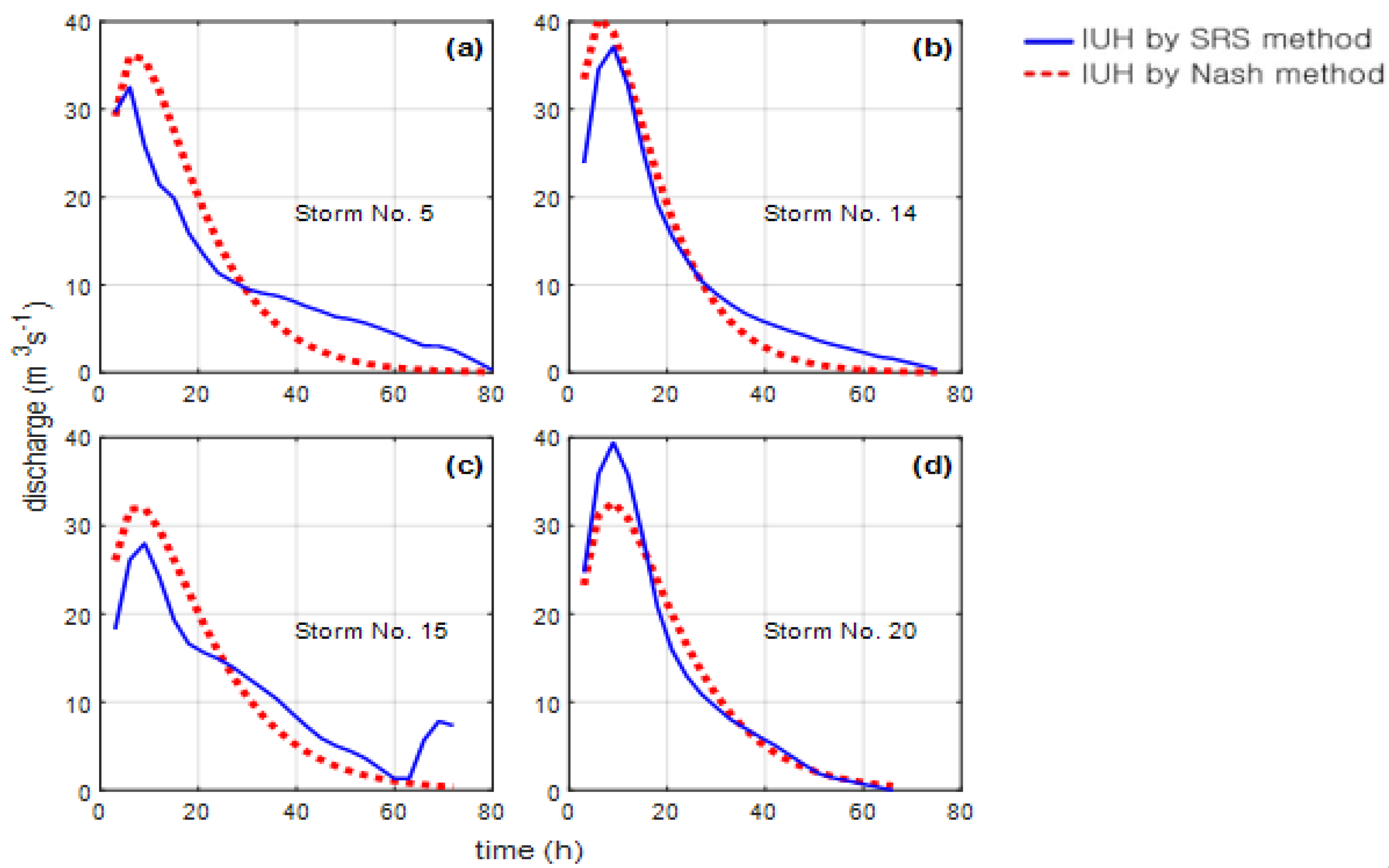
Since numerical comparison is difficult, Figure 3 compares the IUH ordinates for the four selected storms [1,11].
In theory, the ordinate of an IUH at time t is the slope of the S-curve of intensity 1 cm/h at the corresponding time. If the time interval of ordinates of the S-curve is infinitesimal, the slope is equivalent to the differentiation. In this study, the differentiation of S ^ ( z 1 ) is performed by the digital filtering method as well as the method of a prior research [1], which uses the Savitzky-Golay smoothing and differentiation filter. These IUHs based on the SRS method were compared with Nash IUHs reported in the literature [11]. The Nash IUH is represented in Equation (22).
h ( t ) = 1 K Γ ( n ) ( t K ) n 1 e t K
where h ( t ) is the IUH ordinates at time t, n, and K are parameters that define the shape and scale of the Nash IUH. The Nash IUH requires a complete set of rainfall–runoff data to obtain the model parameters.
In Figure 3, the values of the time-to-peak of IUH based on the SRS method appear to be very similar (within single time step of calculation) to those of the Nash IUHs in all selected cases. The rising and falling limbs of the proposed IUH are underestimated near the peak of the Nash IUH for each storm event except storm event 20. To check the performance index of STDER, the Nash IUH is adopted as the reference IUH. The STDER of each storm is listed in Table 2 along with the adopted parameter values to set up the Nash IUH [11].
Table 2 indicates that when the SRS is applied to each storm, the estimated IUHs are generally in good agreement. Interestingly, storm event 20 shows the smallest STDER even if it provided rather poor accuracy in estimating the peak value.
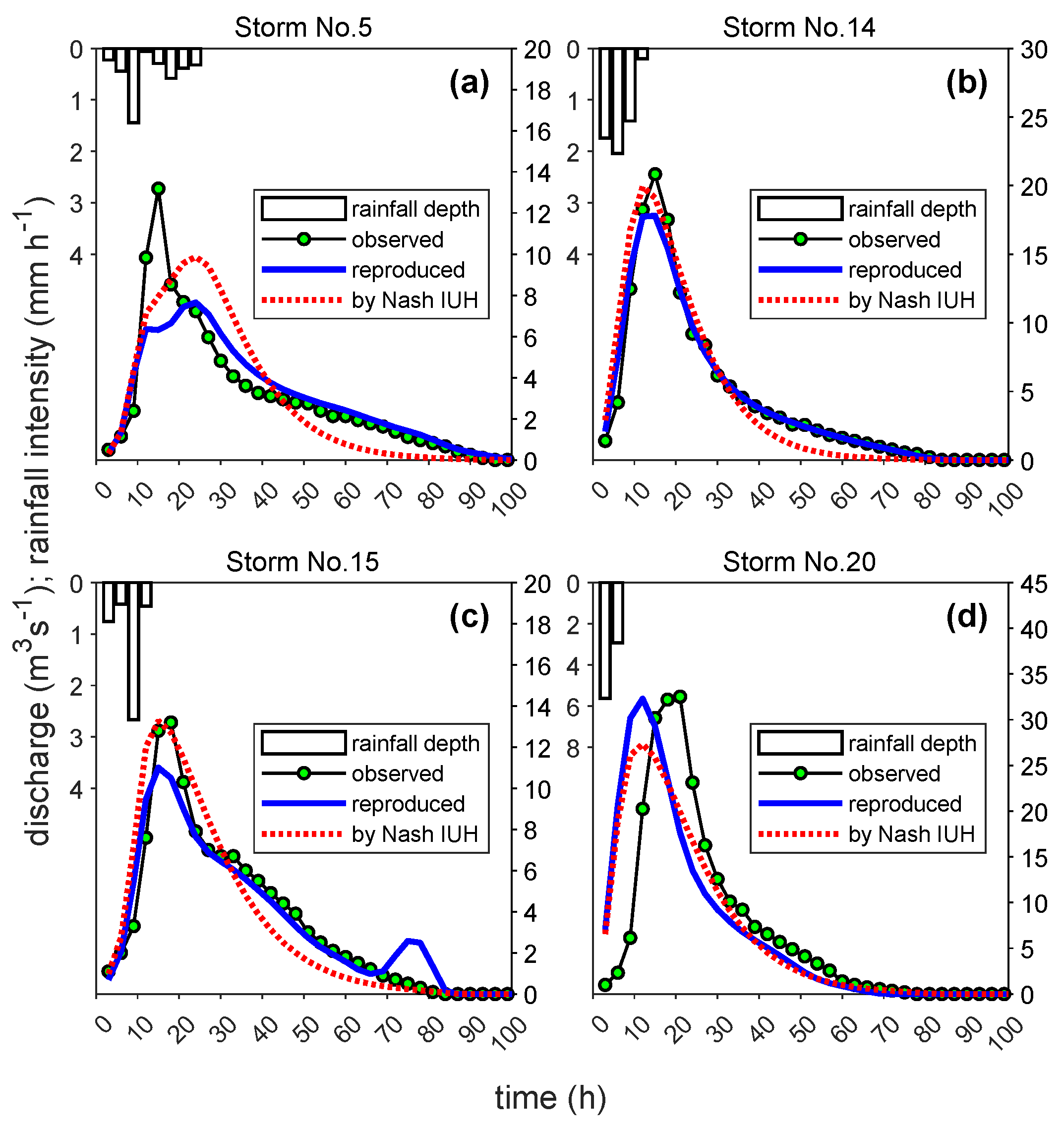
A plot showing the comparison between the observed and reproduced discharges for the four storms is presented in Figure 4.
When the SRS method is applied to measured rainfall-runoff data, the estimated UHs should be consistent with the UHs resulting from the conventional method to provide reproduced flows close to the measured runoff. An overview of runoff reproduction by SRS is presented to appreciate the advantage of the SRS method. For given storm events, the calculated results listed in Table 2 are compared through the Nash-Sutcliffe model efficiency coefficient formulated in Equation (20) and the peak relative error formulated in Equation (21). It can be clearly observed from Figure 4 as well as Table 1 that the UH based on the SRS method reproduced runoff responses very close to the observed runoff hydrograph, while the reproduced runoff responses are not consistent with the observed ones for storm events 5 and 20 by showing E = 77.6% and 40.2%, respectively. The reproduced runoff generally underestimates within a narrow range, which is between 0.007 and 0.420. However, the simulated runoff using the Nash model provided in prior research [11] shows virtually consistent results with the runoff responses using the SRS method. The reproduced runoffs for four storms were computed for the Nash model, and the results were compared with those of the SRS method in Figure 4 and listed in Table 2. The figure shows that the reproduced ordinates by the SRS method and Nash model agree well with each other. Interestingly, although it is not a remarkable difference in values, the SRS method shows a better or comparable E value than the Nash model, even though the SRS method is a restricted method not using rainfall information. However, the SRS method is far less sensitive to fit the peak ordinate of measured runoff than the Nash model when comparing QBs in Table 2. As long as accurately measured effective rainfall and direct runoff are used, the reproduced runoff will be consistent with the result of existing UH model, as seen in the case of storm event 14. The discrepancy of storm event 15 is due to the oscillation of the S-curve. This will be discussed in detail in the discussion section. The problem of event 20 can be resolved if a delay is given to S-curve. In Figure 1, the point z−1 = 0 represents unit delay, and this delay is equally applied to each event. Therefore, this discrepancy problem of storm event 20 appears to be caused by the nonlinearity of this event. Thus, the inconsistency problem of storm events 5 and 20 is not inherent to the proposed method itself, but it is associated with the fundamental problem related to the nonlinearity of the system, the base-flow separation, and infiltration for these storms. It is an important aspect of the SRS method which can give information on the usefulness level of the rainfall-runoff data we are dealing with.

4. Discussion

4.1. Comparison of Argand Diagrams

The conventional RS method [6] determines the roots of the UH polynomial H ( z 1 ) , in which H ( z 1 ) is the Z-transform of h ( t ) in Equation (11). In the present method, the selection of the UH roots is performed based on the a priori expectation that the roots will draw a skewed circle in the Argand diagram. The Argand diagrams of storm events 5, 14, 15, and 20 are plotted in Figure 5.
All the storm events in Figure 5 show a number of roots of the polynomial H ( z 1 ) lying outside the expected ideal skewed circle. The skewed circles are not easily identifiable for storm events 15 and 20 in Figure 5c,d, respectively. Furthermore, the abnormal roots, representing the roots of effective rainfall polynomial X ( z 1 ) can be over-counted according to the researcher’s subjective decision. These over-counted roots sometimes produce a higher degree polynomial X ( z 1 ) than the actual one, and they may lead to unrealistic effective rainfall distribution. Furthermore, the relevant UH polynomial is never stable unless smoothing methods are additionally introduced into the RS procedure. In contrast, the proposed method differs from the conventional method in that SRS makes it possible to separate clearly X ( z 1 ) from runoff, as shown in Figure 1. In fact, the SRS method automatically separates X ( z 1 ) from R ( z 1 ) prior to the analysis. Naturally, the coordinates of roots for X ( z 1 ) obtained by SRS are completely included in the roots of the RS method. This explains that SRS does not affect X ( z 1 ) of the RS method. Therefore, it is reasonable to suppose that SRS is more objective by reducing some ambiguity in separating transfer functions from runoff data.
Unusual rainfall pattern, errors in the baseflow separation method, and measurement error may result in a pattern of chaotically scattered roots. As a result, the S-curve oscillates rather than approaching an equilibrium value and can produce largely erroneous ordinates at the tail. As mentioned earlier, the circle pattern of roots is not more easily identifiable for storm event 15, as seen in Figure 5c. This leads to the oscillations of the S-curve. In this study, an attempt was made to stabilize the oscillations occurring at the ends of the S-curve using a simple linear programming method, but it did not give better results than those shown in Figure 2c. Therefore, the S-curve needs to be smoothened graphically before taking derivatives to give better results than the IUH and runoff predictions shown in Figure 3c and Figure 4c, respectively.

4.2. Examples for Different River Basins

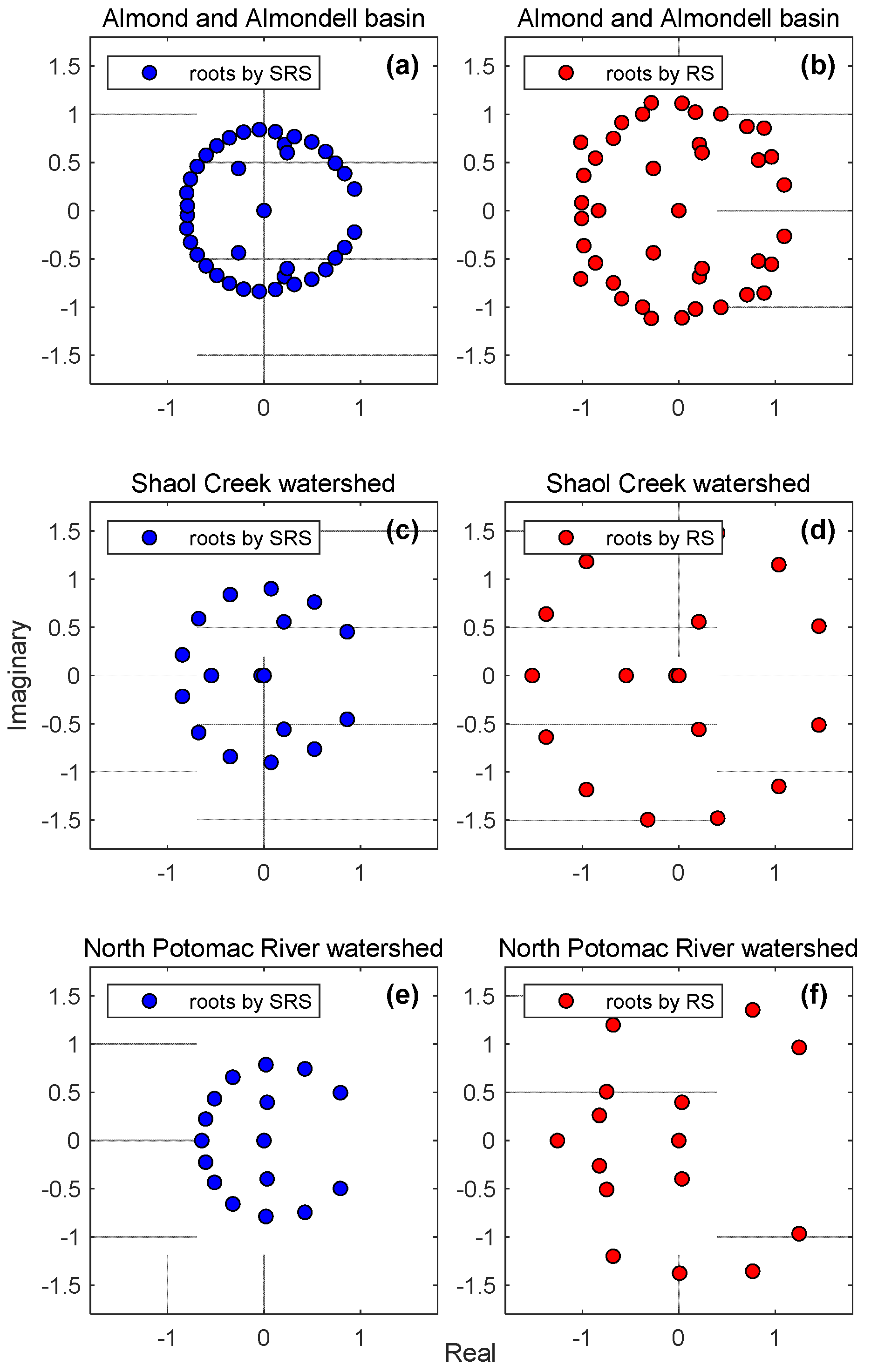
To evaluate the generality of the SRS method, additional analyses for the storms of other basins were carried out. For this, Argand diagrams for direct runoff of the three different river basins using the SRS method were compared to the results obtained by the RS method. The basins considered here are dealt in the previous study [1] by the authors, and they show a wide range of watershed areas. The first result is from the storm event occurring in the Almond and Almondell catchment (229 km2), U.K. [18]; the second result is obtained using a storm event in the Shaol Creek watershed (11.25 km2), USA [5]; the third result is obtained based on the runoff data of the North Potomac River watershed (2266 km2), USA [19]. The complex roots for each basin resulting from both SRS and RS methods are plotted on Argand diagrams in Figure 6.
From Figure 6, it appears clearly that the SRS method leads to an apparently better separation of hydrologic response than the RS method in each considered basin, as observed previously in the Nenagh basin. As a result, the roots corresponding to the S-curve and rainfall can be readily identified in each basin when using SRS. Another advantage is that the specific hydrologic response feature of each basin can be readily distinguished from each other when the SRS method is used. The left panels of Figure 6 show that the position of the circular pattern of roots differs slightly in each case. This implies that there exists a specific root pattern of hydrologic response in each basin. This can be identified in the Nenagh basin cases by showing the roots pattern of S-curves to be virtually identical to each other, as illustrated in Figure 1. In fact, a similar result has already been revealed in a previous study [6] using RS. However, SRS provides better results than using the RS method.

4.3. Consideration of Stability Using Argand Diagram

In the frequency domain, the system response functions, such as S-curve or UH, are given by the quotient obtained when dividing the input (rainfall) by the output (CFR or runoff). Therefore, the coefficients of these functions are positive and real. The system response (S-curve) can be given by rearranging Equation (6), which leads to
S ( z 1 ) = R ( z 1 )   X ( z 1 ) = r 1 z 1 +     + r P 1 z ( P 1 ) + r P z P x 1 z 1 +     + x M 1 z ( M 1 ) + x M z M .
For a stable hydrological system, the zero-crossings of the polynomial denominator must be equal to those of the polynomial numerator; otherwise, the system cannot be stable because of the occurrence of oscillations in the system responses. The zero-crossings of the numerator and denominator polynomials in Equation (23) are conjugate complex numbers. In the SRS or RS method, the polynomial denominator of Equation (23) is a mathematical rainfall polynomial X m a t h ( z 1 ) of which the zero-crossings are those of the polynomial numerator. In a previous study [20], this X m a t h ( z 1 ) was used as a replacement of the observed rainfall polynomial X o b s ( z 1 ) to get complete stability of the system. However, it is hardly hydrologically justifiable unless the roots of X m a t h ( z 1 ) are close to those of X o b s ( z 1 ) . However, instead of using this replacement method, using the least square method with an average rainfall of X m a t h ( z 1 ) and ( z 1 ) seems to be more rational if hydrologic restrictions such as infiltration assumptions or continuity condition are a priori considered. In this case, stability can be achieved by using S-curve smoothing [1,20].
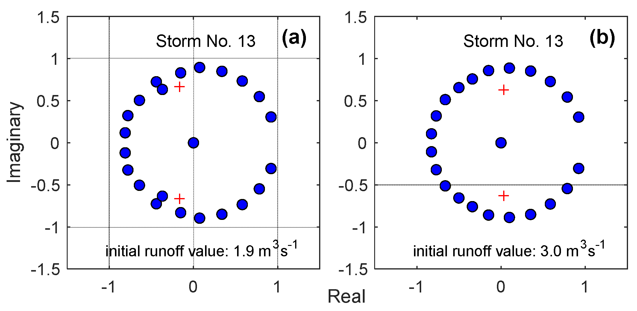
In order to investigate the hydrologic restrictions, the effect of a small difference in the runoff value on the hydrologic stability is examined. To do this, this study selected an event where the real part of the rainfall roots is negative. For example, for storm event 13 in Table 1, increasing the initial non-zero runoff value (=ordinate at t = 3   h ) by 1.1 m3s−1 from 1.9 to 3.0 m3s−1 produces the circle pattern of the runoff polynomial shown in Figure 7. The increased runoff value is at most 4% of the peak flow rate (25.32 m3s−1), but it can be seen from Figure 7 that a hydrologically sensitive change occurs.
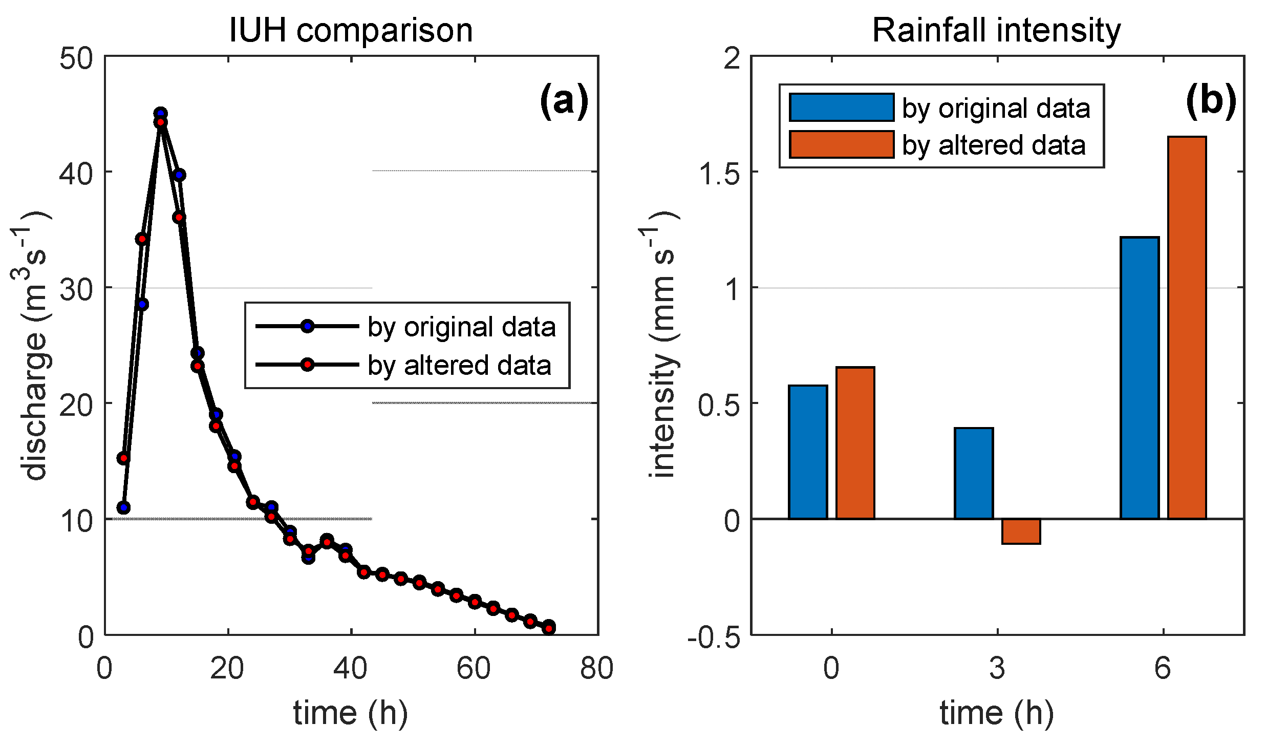
By performing this alteration, the root patterns of the S-curve polynomial H ( z 1 ) become closer to a smoother circle for the initial runoff of 3.0 m3s−1, as shown in Figure 7a,b. Even so, this small variation of initial runoff value does not affect significantly the root pattern of S ( z 1 ) . This is thought to be because a large number of S-curve ordinates share the alteration of runoff. Accordingly, both IUHs are readily identical, as shown in Figure 8a.
However, the result for rainfall polynomial X ( z 1 ) is quite different from that of the S-curve. The coefficient of the first-order term in polynomial X ( z 1 ) changed from 0.3322 to −0.0640. As a result, the rainfall intensity after altering runoff has a negative value, as can be seen in Figure 8b. This change in sign is due to the shift of the positions of the roots of X ( z 1 ) on the positive real axis resulting from the alteration of the initial runoff value. This may violate the hydrologic stability condition. However, if this negative value is considered to have occurred due to a very high rate of surface evaporation in the middle of a complex rainfall event, the hydrologic stability conditions can be satisfied [21]. However, relating directly a high rate of evaporation occurring during a storm to the alteration of initial runoff seems quite delicate. Rather, this case seems to be more related to the method of calculating the direct runoff from a measured runoff. Such a negative coefficient in polynomial X ( z 1 ) can happen because a small amount of variation for runoff is acceptable when considering the common base flow separation process. Thus, it is recommended to derive the response functions with caution by referring to the SRS method proposed in this study.

5. Conclusions

This paper suggested a reliable method that can be used to estimate the S-curve in an objective manner from storms with unreliable rainfall data. This method depends only on the separation of an S-curve from the runoff data of a given basin similar to the root selection method. As an analysis input, cumulative runoff is used to promote less subjectivity in separating the roots of the S-curve and rainfall from the input approximated by power series expansion. This method was designed to outperform the root selection method, so that it was possible to extract the S-curve clearly by avoiding the unclear roots, and to solve the hydrologic stability problem. The applicability of the proposed approach was demonstrated for the Nenagh River basin. Based on the results, the following conclusions can be drawn:
(1)
The proposed method provided a clear and effective tool identifying the S-curve solely from the effective runoff of given storm data.
(2)
The roots of the S-curve polynomial described a clearer circular pattern that allowed root separation for the polynomial without any additional efforts.
(3)
The proposed method did not affect the root pattern of rainfall provided by the root selection method
(4)
The estimates of IUHs were in general agreement with those of previous studies.
(5)
The ordinates of the reproduced direct runoff were in good agreement with those of previous studies.
(6)
Hydrologic stability evaluation could be performed by comparing the roots of observed rainfall and abnormal roots on the Argand diagram.
(7)
The sensitivity of roots for rainfall was relatively larger than that of the S-curve polynomial with respect to a small variation of initial runoff ordinate.

Author Contributions

Conceptualization, K.-W.S.; methodology, K.-W.S.; writing—original draft preparation, K.-W.S. and J.H.S.; writing—review and editing, J.H.S.; project administration, K.-W.S. All authors have read and agreed to the published version of the manuscript.

Funding

This Research was fully funded by a Konkuk University Research Committee grant.

Institutional Review Board Statement

Not applicable.

Informed Consent Statement

Not applicable.

Conflicts of Interest

The authors declare no conflict of interest.

References

  1. Seong, K.-W.; Sung, J. Derivation of S-Curve from Oscillatory Hydrograph Using Digital Filter. Water 2021, 13, 1456. [Google Scholar] [CrossRef]
  2. Patil, P.R.; Mishra, S.K. Analytical Approach for Derivation of Oscillation-Free Altered Duration Unit Hydrographs. J. Hydrol. Eng. 2016, 21, 06016010. [Google Scholar] [CrossRef]
  3. Hunt, B. The meaning of oscillations in unit hydrograph S-curves. Hydrol. Sci. J. 1985, 30, 331–342. [Google Scholar] [CrossRef] [Green Version]
  4. Parmentier, B.; Dooge, J.; Bruen, M. Root selection methods in flood analysis. Hydrol. Earth Syst. Sci. 2003, 7, 151–161. [Google Scholar] [CrossRef] [Green Version]
  5. Prasad, T.D.; Gupta, R.; Prakash, S. Determination of Optimal Loss Rate Parameters and Unit Hydrograph. J. Hydrol. Eng. 1999, 4, 83–87. [Google Scholar] [CrossRef]
  6. Turner, J.; Dooge, J.; Bree, T. Deriving the unit hydrograph by root selection. J. Hydrol. 1989, 110, 137–152. [Google Scholar] [CrossRef]
  7. Al-Dabbagh, A.R. Mathematical Model To Simulate The Surface Runoff For Ubaiyidh Valley In The Western Desert. Eng. J. Univ. Quatar 1998, 11, 153–167. [Google Scholar]
  8. Seong, K.-W.; Lee, Y.-H. A practical estimation of Clark IUH parameters using root selection and linear programming. Hydrol. Process. 2011, 25, 3676–3687. [Google Scholar] [CrossRef]
  9. Rai, R.K.; Jain, M.K.; Mishra, S.K.; Ojha, C.S.P.; Singh, V.P. Another Look at Z-transform Technique for Deriving Unit Impulse Response Function. Water Resour. Manag. 2007, 21, 1829–1848. [Google Scholar] [CrossRef]
  10. Bree, T. The stability of parameter estimation in the general linear model. J. Hydrol. 1978, 37, 47–66. [Google Scholar] [CrossRef]
  11. Mohan, S.; Vijayalakshmi, D.P. Estimation of Nash’s IUH parameters using stochastic search algorithms. Hydrol. Process. 2008, 22, 3507–3522. [Google Scholar] [CrossRef]
  12. James, G.; Burley, D.; Clements, D.; Dyke, P.; Searl, J. Modern Engineering Mathematics; Pearson Education: Essex, UK, 2008. [Google Scholar]
  13. Sharma, T. Response functions applied to a drainage system. J. Hydrol. 1980, 45, 279–287. [Google Scholar] [CrossRef]
  14. Bhunya, P.K.; Ghosh, N.C.; Mishra, S.K.; Ojha, C.S.; Berndtsson, R. Hybrid Model for Derivation of Synthetic Unit Hydrograph. J. Hydrol. Eng. 2005, 10, 458–467. [Google Scholar] [CrossRef]
  15. Nash, J.; Sutcliffe, J. River flow forecasting through conceptual models part I—A discussion of principles. J. Hydrol. 1970, 10, 282–290. [Google Scholar] [CrossRef]
  16. Reddy, J.M.; Babu, A.S.; Mallikarjuna, C. Rainfall—Runoff Modeling: Comparison and Combination of Simple Time-Series, Linear Autoregressive and Artificial Neural Network Models. WSEAS Trans. Fluid Mech. 2008, 3, 126–136. [Google Scholar]
  17. Cleveland, T.G.; He, X.; Asquith, W.H.; Fang, X.; Thompson, D.B. Instantaneous Unit Hydrograph Evaluation for Rainfall-Runoff Modeling of Small Watersheds in North and South Central Texas. J. Irrig. Drain. Eng. 2006, 132, 479–485. [Google Scholar] [CrossRef]
  18. Zhao, B.; Tung, Y.-K.; Yang, J.-C. Estimation of Unit Hydrograph by Ridge Least-Squares Method. J. Irrig. Drain. Eng. 1995, 121, 253–259. [Google Scholar] [CrossRef] [Green Version]
  19. Bhattacharjya, R.K. Optimal design of unit hydrographs using probability distribution and genetic algorithms. Sadhana 2004, 29, 499–508. [Google Scholar] [CrossRef]
  20. Lattermann, A. System-Theoretical Modelling in Surface Water Hydrology; Springer Series in Physical Environment; Springer: Berlin/Heidelberg, Germany, 1991; Volume 6, ISBN 978-3-642-83821-7. [Google Scholar]
  21. Turner, J.E.; Dooge, J.C.I.; Bree, T. Comment on Single Storm Runoff Analysis Using Z-Transform. J. Hydrol. Eng. 2001, 6, 173–174. [Google Scholar] [CrossRef]
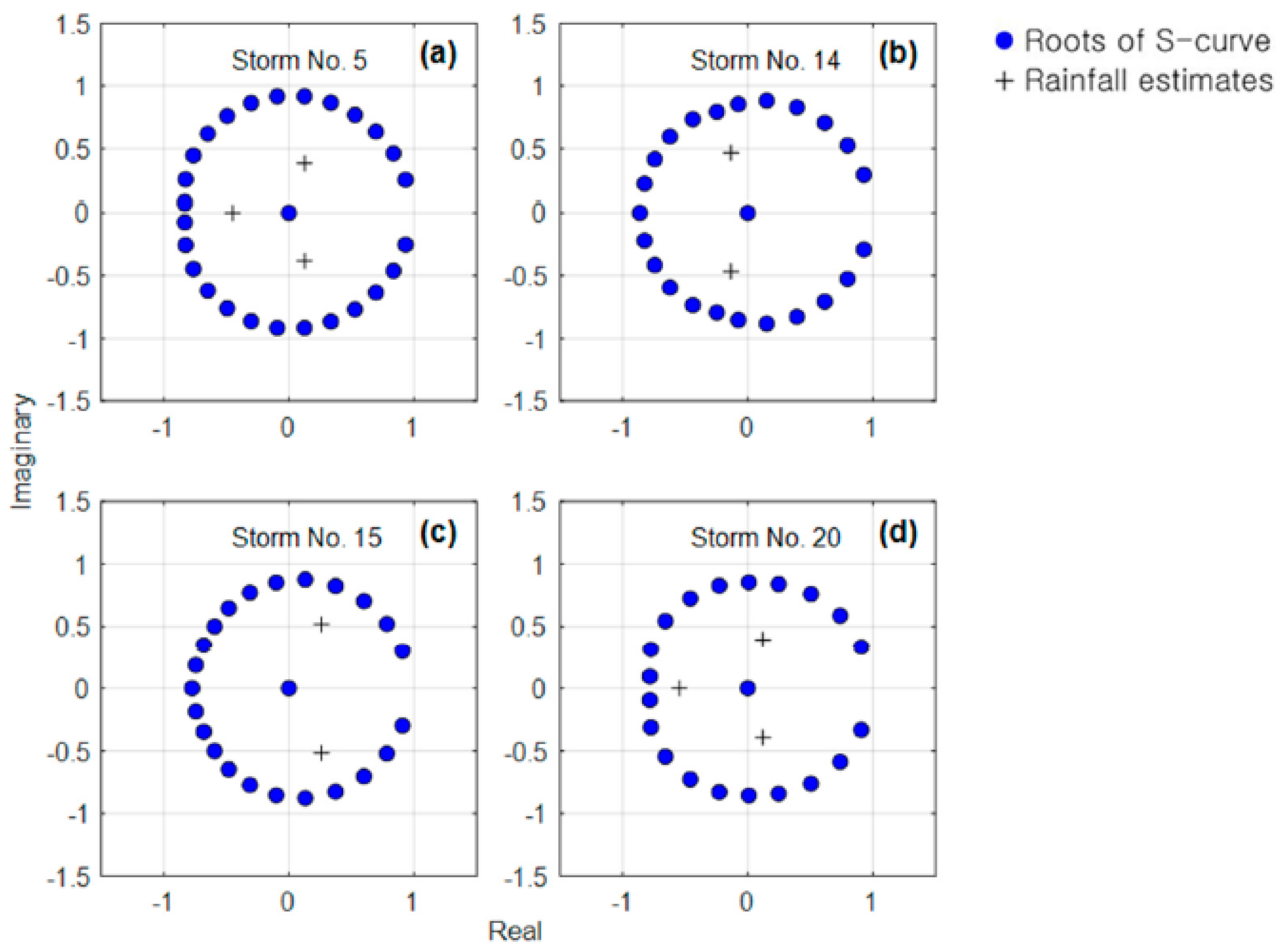
Figure 1. Argand diagrams obtained by the proposed method for selected storms of Nenagh basin: (a) for Storm No. 5; (b) for Storm No. 14; (c) for Storm No. 15; (d) for Storm No. 20.
Water 13 03447 g001
Figure 2. Comparison between S-curves for each storm derived by the SRS method and those based on UH obtained by the least square method using rainfall data: (a) for Storm No. 5; (b) for Storm No. 14; (c) for Storm No. 15; (d) for Storm No. 20.
Water 13 03447 g002
Figure 3. Comparison between IUHs for each storm derived by a digital filtering method using the S-curve from the SRS method and Nash IUHs whose parameters are referenced from prior research: (a) for Storm No. 5; (b) for Storm No. 14; (c) for Storm No. 15; (d) for Storm No. 20.
Water 13 03447 g003
Figure 4. Comparison of reproduced runoff with that observed for each storm: (a) for Storm No. 5; (b) for Storm No. 14; (c) for Storm No. 15; (d) for Storm No. 20.
Water 13 03447 g004
Figure 5. Argand diagrams obtained by the conventional RS method for selected storms of Nenagh basin: (a) for Storm No. 5; (b) for Storm No. 14; (c) for Storm No. 15; (d) for Storm No. 20.
Water 13 03447 g005
Figure 6. Comparison between Argand diagrams of the storms for different three basins obtained by the SRS method (left panel of each row) and the RS method (right panel of each row): (a,b) for Almond and Almondell basin; (c,d) for Shaol Creek watershed; (e,f) for North Potomac River watershed.
Water 13 03447 g006
Figure 7. Comparison between Argand diagrams for Storm No. 13 of Nenagh basin obtained by altering initial runoff value: (a) for initial runoff of 1.9 m3s−1 (original), (b) for initial runoff of 3.0 m3s−1 (altered).
Water 13 03447 g007
Figure 8. Comparison between IUHs and hyetographs for Storm No. 13 of Nenagh basin obtained by altering initial runoff value: (a) for initial runoff of 1.9 m3s−1 (original), (b) for initial runoff of 3.0 m3s−1 (altered).
Water 13 03447 g008
Table 1. Characteristic of selected storm events in the Nenagh basin.
Event NumberTime to Peak (h)Peak Flow Rate (m3s−1)Base Time (h)
51513.1993
131525.3278
141520.8481
151813.2081
202123.5275
Average16.8019.2181.6
Sources: Bree (1978) [10]; Mohan and Vijayalakshmi (2008) [11].
Table 2. Nash IUH parameters, STDER, and QB for the selected storm events of Nenagh basin.
Event NumbernKSTDER
(%)
EQB
Nash Model
(%)
SRS Method
(%)
Nash ModelSRS Method
51.7793.0505.6767.177.60.2520.420
141.8082.07053.7991.097.10.0440.145
151.6923.6054.6283.390.8−0.0060.167
201.8673.2593.2360.540.20.1590.007
Publisher’s Note: MDPI stays neutral with regard to jurisdictional claims in published maps and institutional affiliations.