Article

Comparison of Machine Learning Algorithms for Discharge Prediction of Multipurpose Dam

1
Department of Earth and Environment, Boston University, Boston, MA 02215, USA
2
Department of Regional Infrastructure Engineering, Kangwon National University, Chuncheon-si 24341, Korea
3
Korea Water Environment Research Institute, Chuncheon-si 24408, Korea
*
Author to whom correspondence should be addressed.
Water 2021, 13(23), 3369; https://doi.org/10.3390/w13233369
Submission received: 17 October 2021 / Revised: 17 November 2021 / Accepted: 25 November 2021 / Published: 29 November 2021
(This article belongs to the Section Hydrology)

Abstract

:
For effective water management in the downstream area of a dam, it is necessary to estimate the amount of discharge from the dam to quantify the flow downstream of the dam. In this study, a machine learning model was constructed to predict the amount of discharge from Soyang River Dam using precipitation and dam inflow/discharge data from 1980 to 2020. Decision tree, multilayer perceptron, random forest, gradient boosting, RNN-LSTM, and CNN-LSTM were used as algorithms. The RNN-LSTM model achieved a Nash–Sutcliffe efficiency (NSE) of 0.796, root-mean-squared error (RMSE) of 48.996 m3/s, mean absolute error (MAE) of 10.024 m3/s, R of 0.898, and R2 of 0.807, showing the best results in dam discharge prediction. The prediction of dam discharge using machine learning algorithms showed that it is possible to predict the amount of discharge, addressing limitations of physical models, such as the difficulty in applying human activity schedules and the need for various input data.

1. Introduction

Water management is one of the most important preparations for a rapidly changing climate. As climate change progresses, there will be greater variability of floods and droughts, occurring more frequently and longer; thus, water resource management will become more important [1]. Dams are built for various purposes such as a stable supply of water resources and flood control [2,3,4]. Since the amount of discharge from dams for various purposes greatly affects the water quality and ecosystem, as well as the water quantity of downstream rivers, research on the amount of discharge from the dam is very important for water management [5,6]. Furthermore, discharging the appropriate amount at the right time is required for preventing droughts and floods. Especially in Korea, where rainfall is concentrated in the summer, a water resource and ecosystem management plan in the downstream water system should be systematically established in advance by predicting the amount of discharge from the upstream multipurpose dam. For this purpose, there is a need for a method that can efficiently predict the amount of discharge from multipurpose dams mediated by artificial effects.
Research on the estimation of the inflow and discharge of dams has been being conducted using various methods involving physical hydrological models such as SWAT, HEC-HMS, and HSPF. The Shetran model for the discharge of the Yangze River at the Three Gorges Dam allowed predicting the future discharge using future climate data [7]. The effect of discharge from the Geumgangsan Dam on the downstream river was analyzed using the SWAT model [8].
For the discharge estimation, since the discharge of multipurpose dams is controlled by human manipulation, reflecting various influencing factors such as precipitation, dam level, and downstream river regimes, it is difficult to collect data on a fixed dam operation schedule. In addition, uncertainties in the calibration parameters of physical hydrologic models can affect the estimate of discharge.
The research method using machine learning has the advantage of being easy to run because it requires less diverse data than a physical model. Therefore, several researchers have researched water resources by applying machine learning due to the convenience of machine learning models, which do not require the professional knowledge of hydrological phenomena and complete input data for each step of physical models. The inflow of a dam was simulated using six machine learning algorithms, and the algorithms were combined for inflow estimation [9]. Furthermore, the forecasting models for the daily water level of the Klang Gate Dam were constructed using a timeseries regression model and support vector machine [10]. Real-time flood discharges upstream and downstream of a multipurpose dam were also forecasted using gray models [11]. Machine learning has presented the advantages of accessibility, as well as higher model accuracy, in several studies [12,13].
With machine learning, it is expected to be able to easily simulate the amount of discharge from a multipurpose dam. However, there has not been a comparative analysis of the performance of various machine learning models to predict the amount of discharge from multipurpose dams.
Therefore, in this study, the discharge of the Soyang River Dam was predicted using various machine learning algorithms. The aim of this study was to explore the optimum algorithm for the prediction of discharge of the Soyang River Dam for an efficient water management and agricultural water management plan in the downstream area of the dam.

2. Materials and Methods

2.1. Study Area

The Soyang River Dam is located upstream of the Bukhan River, which is one of the main tributaries of the Han River Basin in South Korea (Figure 1). The area of the watershed of the Soyang River Dam is 2637 km2, consisting of forest area (89.5%), agricultural land (5.7%), water (2.4%), and other land uses (2.4%). The annual precipitation at the Chuncheon weather station was 1327 mm on average, varying between 677.0 mm and 2069 mm from 1980 to 2020. The annual precipitation at the Inje weather station was 1778.5 mm on average, varying between 666.9 mm and 1185.6 mm from 1980 to 2020 [14].
The Soyang River Dam is a multipurpose dam with a total storage capacity of 2900 million tons, an effective storage capacity of 1900 million tons, and an annual water supply of 1213 million tons [15]. The Soyang River Dam discharges to control the water level, supply water downstream, and generate electricity. As unexpected climate events occur more frequently, daily planning for discharge through systematic management can prevent disasters caused by floods and droughts.

2.2. Data Descriptions

In this study, the precipitation data observed from 1980 to 2020 at the Chuncheon weather station and Inje weather station, as well as the inflow and discharge of the Soyang River Dam, were used to develop the machine learning models.
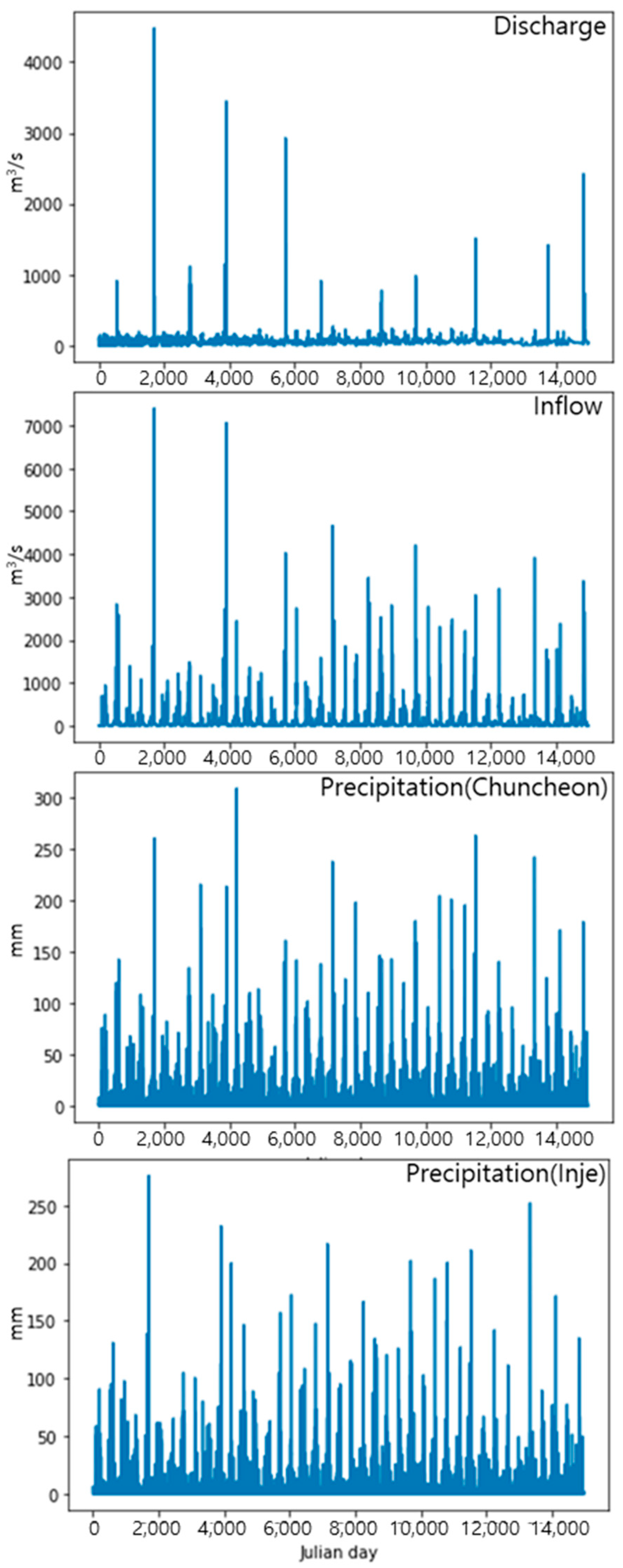
The precipitation data were obtained from the Korea Meteorological Administration database for the Chuncheon weather station and Inje weather station [14]. The Chuncheon weather station is located near the outlet of the Soyang River Dam, and the Inje weather station is located in the Soyang River Dam basin. The discharge and the inflow data of the Soyang River Dam were obtained from the Korea Water Resources Corporation (K-water) [15]. Figure 2 shows the data used for the discharge prediction with temporal variation in the dam discharge (m3/s), dam inflow (m3/s), and precipitation (mm). The other weather data such as temperature, humidity, wind speed, and solar radiation were not chosen as features for discharge prediction, since the data showed a poor correlation with the discharge of the Soyang River Dam.
For the discharge prediction model construction, precipitation data of the day (forecasted), precipitation data of 1 day ago, precipitation data of 2 days ago, the inflow of 1 day ago, the inflow of 2 days ago, the discharge of 1 day ago, and the discharge of 2 days ago from 1 January 1980 to 31 December 2020 were used (Table 1). A widely used method for calculating effective rainfall is the NRCS method using 5 day antecedent rainfall; however, it is applicable for watersheds in the United States. A study found that the preceding 2 day rainfall gave the most suitable results in Korean watersheds [16]; thus, preceding 2 day rainfall was used in this study. According to a study conducted in an alpine headwater catchment, soil moisture affects runoff [17]. Therefore, the historical precipitation data were used to simply reflect the soil moisture of the day.
In this study, the scaling method and standardization methods included shape scaling, normalization, and standardization using the ‘StandardScaler’ function from ‘sklearn.preprocessing’ library for a preprocessing step for data preprocessing. Data preprocessing needs to be performed for effective machine learning to improve the quality of data and to generate comprehensible information.

2.3. Machine Learning Algorithms

In this study, six machine learning models were created to estimate the discharge amount of the Soyang River Dam.
Machine learning algorithms learn and improve model performance via training using data. Machine learning is categorized as supervised learning, unsupervised learning, or reinforcement learning [18], and the algorithms for this study were supervised learning methods that used labeled data. Information about each model is given in Table 2.

2.3.1. Decision Tree

A decision tree is an algorithm for classification and regression, and it makes decisions by continuously asking yes or no questions [19]. In the decision tree, the hyperparameter stops the tree before it is completely constructed as the pre-pruning parameter. For the decision tree model, ‘max_depth’, ‘max_leaf_nodes’, or ‘min_samples_leaf’ parameters are designated for preventing overfitting. The decision tree in the scikit-learn is intended to provide adequate prefabrication through ‘min_samples_leaf’. Other variables are shown in Table 3: entropy for criterion, 1 for min_samples_leaf, 0 for min_impurity_decrease, best for splitter, 2 for min_samples_split, and 0 for random_state.

2.3.2. Multilayer Perceptron

Multilayer perceptron (MLP) is a feed-forward neural network. MLP consists of an input layer, a hidden layer, and an output layer. The input data is entered into the input layer and weighted according to the set hidden layer structure; then, the result is printed by the output layer [20]. MLPs with hidden layers produce more accurate predictions than other machine learning techniques [21]. Table 3 provides details on the hyperparameter settings of the MLPRegressor function. The most important hyperparameter is the hidden layer configuration, with 50 nodes in each of the three layers. The critical hyperparameters in the MLP regressor were as follows: 50 nodes for each of the three layers for hidden_layer_sizes, adam for solver, 0.001 for learning_rate_init, 200 for max_iter, 0.9 for momentum, 0.9 for beta_1, 1 × 10⁻⁸ for epsilon, and relu for activation.

2.3.3. Random Forest

Random forest is a classification technique that combines a bagging algorithm, an ensemble learning method, and a classification and registration tree (CART) algorithm [22]. The performance of RF is strong in prediction including many variables of low importance [23]. Furthermore, RF is an algorithm that provides good results with the default settings [24]. Among the hyperparameters set in the ‘RandomForestRegressor’ function used in this study, the sensitive hyperparameter was the basic parameter. Since the random forest model is an ensemble model of decision trees, the default parameter was the tree number ‘n-estimator’ and the value was set to 50. The other variables were 2 for min_samples_split, 0 for min_weight_fraction_leaf, 0 for min_impurity decrease, 0 for verbose, mse for criterion, 1 for min_samples_leaf, auto for max_features, and true for bootstrap (Table 3).

2.3.4. Gradient Boosting

Gradient boosting is an ensemble model that learns a boosting algorithm using ensemble learning in a decision tree. In gradient boosting, the gradient exposes the weaknesses of the models trained so far, while other models focus on improving performance. For better prediction, the parameters that minimize the loss function that quantifies the error of the prediction model should be found. The advantage of gradient boosting is that other different loss functions can be used as much as possible. Furthermore, the properties of the loss function are automatically reflected in learning with gradients [25]. The hyperparameters of the GradientBoostingRegressor function are shown in Table 3: 1 s for loss, 100 for n_estimators, friedman_mse for criterion, 1 for min_samples_leaf, 10 for max_depth, 0.9 for alpha, auto for presort, 1 × 10⁻⁴ for tol, 0.1 for learning_rate, 1.0 for subsample, 2 for min_samples_split, and 0.1 for validation_fraction.

2.3.5. LSTM

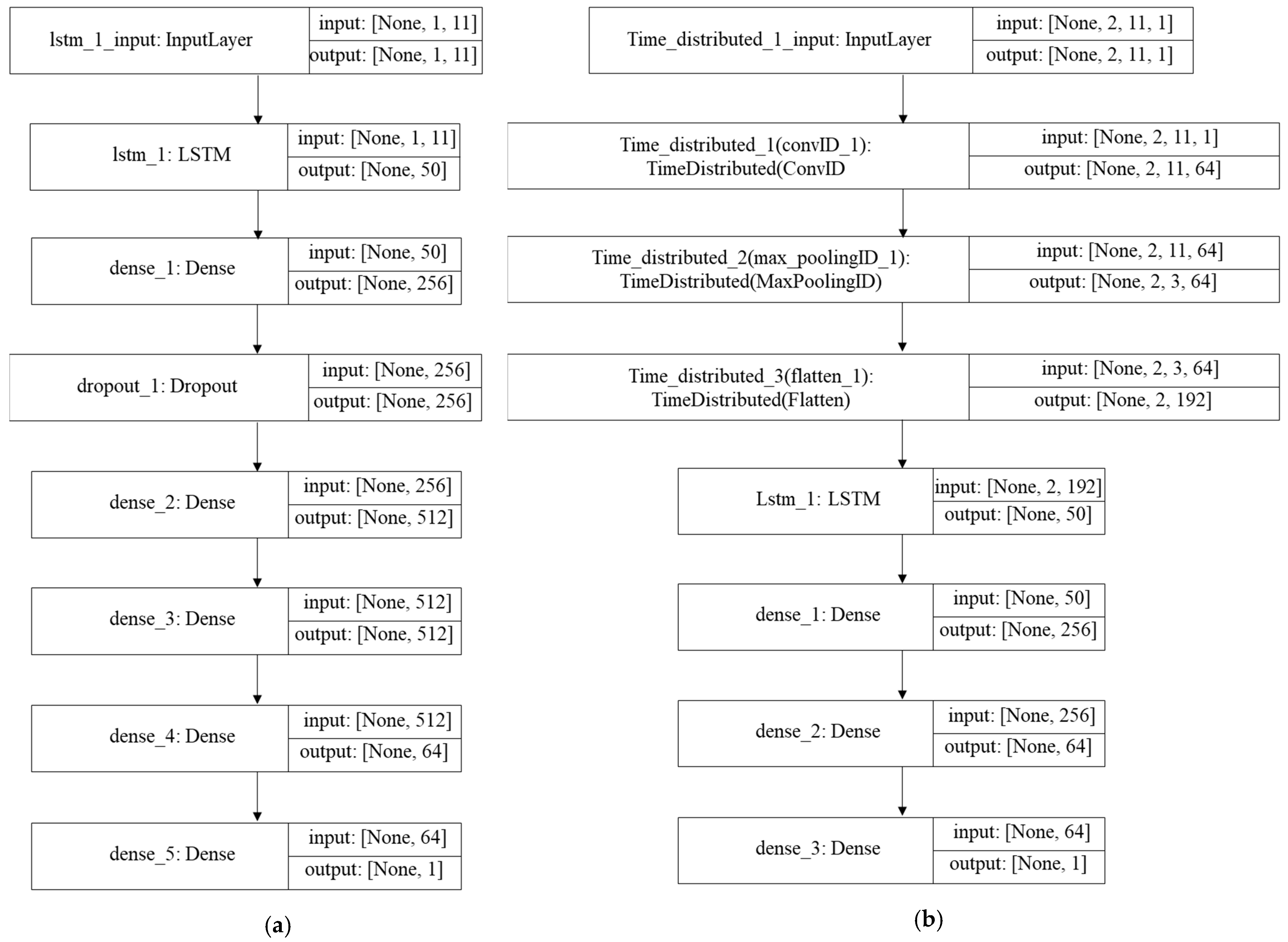
LSTM is an RNN, a kind of deep learning algorithm that repeatedly learns timeseries data [26]. The RNN is a structure where the output data of the previous RNN affect the output data of the current RNN in the data learning process. This allows a link between current and past learning, which is useful for continuous and iterative learning; however, using too much historical data degrades the predictivity of the model. LSTM is a type of RNN-based deep learning algorithm that makes it easy to predict timeseries data by considering the sequencing or temporal aspects of learning and avoiding the chronic weight loss problem of RNNs [27]. In this study, RNN-LSTM incorporated LSTM, dense, and dropout layers to prevent overfitting (Figure 3).

2.3.6. CNN-LSTM

CNN-LSTM is an example of LSTM transformation [28]. As the performance of deep learning has been verified throughout data science and technology, a deep learning technique was designed for solving numerical prediction problems. In this study, the information on the layers added to the sequential functions of RNN-LSTM and CNN-LSTM was composed of seven layers, as shown in Figure 3. RNN-LSTM incorporated LSTM, dense, and dropout layers to prevent overfitting. In the case of CNN-LSTM, CNN, which mainly uses two-dimensional data, can be used for one-dimensional timeseries data to extract data characteristics and analyze data prediction. Additionally, ‘Conv1D’ and ‘MaxPooling1D’ were used to construct the layers for CNN-LSTM.
Figure 4 presents a schematic of this study method.

2.4. Model Training Test

In this study, the discharge of the Soyang River Dam was predicted using weather data and inflow data from the period 1980 to 2020. The model training period was from 1980 to 2015, and the test period was from 2016 to 2020.
To evaluate the performance of each machine learning model, the Nash–Sutcliffe efficiency (NSE), root-mean-squared error (RMSE), mean absolute error (MAE), correlation coefficient (R), and determination coefficient (R2) were used. A significant number of studies have indicated the appropriateness of these measures to assess the accuracy of hydrological models [8,29,30,31]. NSE, RMSE, MAE, R, and R2 for evaluation of the model accuracy were calculated using Equations (1)–(5).
N S E = 1   ( O t   M t ) 2   ( O t   O t ¯ ) 2 ,
R M S E =   ( O t   M t ) 2 n ,
M A E   =   1 n   | M t O t | ,
R   =     ( O t   O t ¯ ) ( M t M t ¯ )   ( O t   O t ¯ ) 2   ( M t   M t ¯ ) 2 ,
R 2   = [   ( O t   O t ¯ ) ( M t M t ¯ ) ] 2   ( O t   O t ¯ ) 2   ( M t   M t ¯ ) 2   ,
where O t is the actual value of t, O t ¯ is the mean of the actual value, M t is the estimated value of t, M t ¯ is the mean of the estimated value, and n is the total number of times.
RMSE is the standard deviation of the residuals, and MAE is the mean of the absolute values of the errors. Therefore, closer verification values to zero denote greater similarity of observed and model values.
R, the correlation coefficient, represents the magnitude of the correlation; R-values are 1, if the observed and simulated values are the same, 0 if they are completely different, and −1 if they are completely the same in the opposite direction. R2 compares the propensity of the observed to the simulated value.

3. Results and Discussion

3.1. Heatmap Analysis

In this study, heatmap analysis was used to evaluate the correlation of the data used (Figure 5). The evaluation showed a correlation coefficient of 0.76 as the highest correlation between the discharge of the day and the discharge of 2 days ago, followed by the discharge of 1 day ago, inflow of 1 day ago, discharge of 1 day ago, inflow of 2 days ago, precipitation of 1 day ago, precipitation of 2 days ago, and precipitation. The results of the heatmap analysis indicated that the discharge and the inflow of the previous days had an impact on the discharge of the multipurpose dam.

3.2. Simulation Results Using Machine Learning Algorithms

Table 4 shows the accuracy (NSE, RMSE, MAE, R, and R2) of the machine learning models by comparing the simulated discharge to the observed discharge. The result from the LSTM model showed the highest accuracy in every measurement for model evaluation with an NSE of 0.796, RMSE of 48.996 m3/s, MAE of 10.024 m3/s, R of 0.898, and R2 of 0.807. Recently, several studies reported the good applicability of LSTM for timeseries streamflow prediction [32,33,34]. The results of this study also showed that the performance of LSTM is good for timeseries hydrologic modeling with good performance in discharge estimation.
The second-best model was RF, with NSE of 678, RMSE of 61.578 m3/s, MAE of 13.058 m3/s, R of 0.840, and R2 of 0.706.
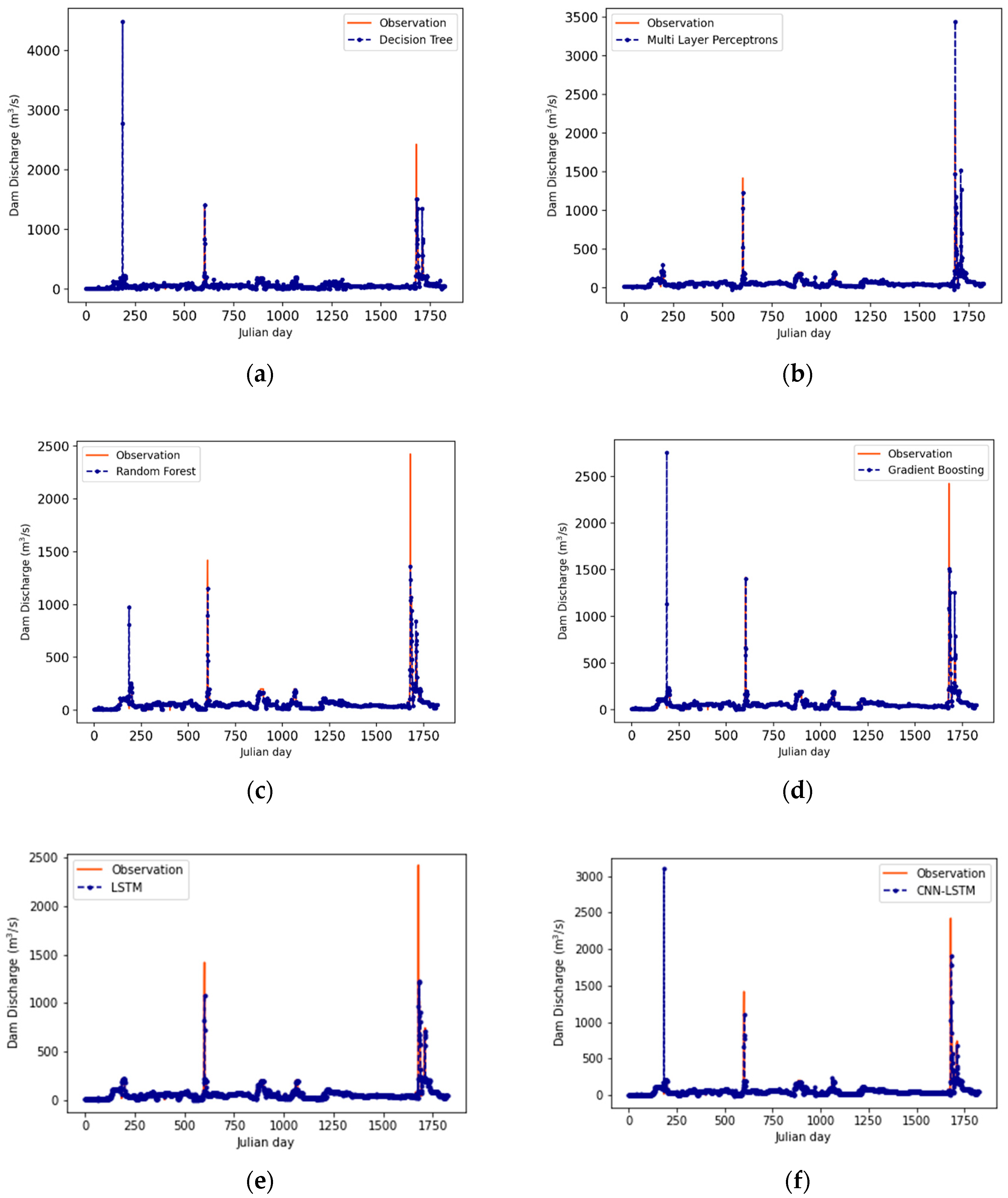
Figure 6 shows that the results from MLP and LSTM predicted the outflow of 6 July 2016, which seemed to be the first peak discharge, whereas the other models overestimated the discharge of 6 July 2016. Unlike the inflow or outflow of a dam that directly discharges the inflow, a multipurpose dam controls the discharge to manage flooding in the downstream area. In the case of general rainfall events, there was a tendency of proportionality to the amount of discharge. However, on 5 July 2016, the amount of precipitation was large, whereas the amount of discharge was small for flood prevention in the downstream areas. MLP and LSTM succeeded in predicting dam discharge control for flood prevention, but the other models failed. The reason for the other peaks shown in Figure 6 is that, on days when there was actually substantial rainfall, a positive rainfall event that would not require dam conditioning for flooding was discharged in proportion to the rainfall. Due to the irregularity of the discharge of the multipurpose dam, most algorithms excluding MLP and LSTM failed to predict the small amount of discharge in high-rainfall events.

4. Conclusions

In this study, machine learning algorithm models to predict the discharge amount of the Soyang River Dam were built, and their performance was evaluated. Machine learning techniques were used to compensate for the shortcomings of hydrologic models, such as data collection of dam operation schedules with human decisions and parameter uncertainty due to human activities.
The results of this study showed that the discharge amount of the Soyang River Dam was effectively simulated using machine learning algorithms. According to the model predictions, LSTM was evaluated to predict the discharge with the best accuracy among the six algorithms used with an NSE of 0.796, RMSE of 48.996 m3/s, MAE of 10.024 m3/s, R of 0.898, and R2 of 0.807, highlighting its success in predicting the irregular pattern of multipurpose dams for functions such as flood control. This result also falls within the range of very good in the hydrological model research accuracy standard [30]. This represents that machine learning models represent a good substitute that can compensate for the limitations of physical hydrologic models in predicting the inflow and discharge of dams. Therefore, it will be possible to prepare plans for droughts and floods by establishing a water supply plan in the downstream area of the dam. Furthermore, unlike existing physical models, only weather data and flow data are required; thus, the applicability of the model will be superior in areas where data acquisition is limited. Therefore, by analyzing the correlation of data and applying an algorithm, it will be possible to promote effective water resource management through flow analysis in the downstream areas of dams in other watersheds. Future research should focus on water resource management in preparation for climate change by constructing a database of flows from worldwide dams using various methods including machine learning models.

Author Contributions

Conceptualization, K.J.L., J.H., J.K. and K.K.; methodology, J.H. and J.H.B.; formal analysis, J.H. and S.L.; data curation, J.H., J.H.B. and D.Y.; writing—original draft preparation, J.H.; writing—review and editing, S.L. and G.L.; supervision, K.J.L. All authors have read and agreed to the published version of the manuscript.

Funding

This research was supported by the Korea Environment Industry and Technology Institute (KEITI) through the Aquatic Ecosystem Conservation Research Program, funded by the Korea Ministry of Environment (MOE), grant number 2020003030004.

Conflicts of Interest

The authors declare no conflict of interest.

References

  1. Hanak, E.; Lund, J.R. Adapting California’s water management to climate change. Clim. Chang. 2012, 111, 17–44. [Google Scholar] [CrossRef]
  2. Hirsch, P.E.; Schillinger, S.; Weigt, H.; Burkhardt-Holm, P. A hydro-economic model for water level fluctuations: Combining limnology with economics for sustainable development of hydropower. PLoS ONE 2014, 9, e114889. [Google Scholar]
  3. Ho, M.; Lall, U.; Allaire, M.; Devineni, N.; Kwon, H.H.; Pal, I.; Raff, D.; Wegner, D. The future role of dams in the U nited S tates of A merica. Water Resour. Res. 2017, 53, 982–998. [Google Scholar] [CrossRef]
  4. Patel, D.P.; Srivastava, P.K. Flood hazards mitigation analysis using remote sensing and GIS: Correspondence with town planning scheme. Water Resour. Manag. 2013, 27, 2353–2368. [Google Scholar] [CrossRef]
  5. Yaghmaei, H.; Sadeghi, S.H.; Moradi, H.; Gholamalifard, M. Effect of Dam operation on monthly and annual trends of flow discharge in the Qom Rood Watershed, Iran. J. Hydrol. 2018, 557, 254–264. [Google Scholar] [CrossRef]
  6. Zhong, Y.; Guo, S.; Liu, Z.; Wang, Y.; Yin, J. Quantifying differences between reservoir inflows and dam site floods using frequency and risk analysis methods. Stoch. Environ. Res. Risk Assess. 2018, 32, 419–433. [Google Scholar] [CrossRef]
  7. Birkinshaw, S.J.; Guerreiro, S.B.; Nicholson, A.; Liang, Q.; Quinn, P.; Zhang, L.; He, B.; Yin, J.; Fowler, H.J. Climate change impacts on Yangtze River discharge at the Three Gorges Dam. Hydrol. Earth Syst. Sci. 2017, 21, 1911–1927. [Google Scholar] [CrossRef] [Green Version]
  8. Lee, G.; Lee, H.W.; Lee, Y.S.; Choi, J.H.; Yang, J.E.; Lim, K.J.; Kim, J. The effect of reduced flow on downstream water systems due to the kumgangsan dam under dry conditions. Water 2019, 11, 739. [Google Scholar] [CrossRef] [Green Version]
  9. Hong, J.; Lee, S.; Bae, J.H.; Lee, J.; Park, W.J.; Lee, D.; Kim, J.; Lim, K.J. Development and evaluation of the combined machine learning models for the prediction of dam inflow. Water 2020, 12, 2927. [Google Scholar] [CrossRef]
  10. Khai, W.J.; Alraih, M.; Ahmed, A.N.; Fai, C.M.; El-Shafie, A. Daily forecasting of dam water levels using machine learning. Int. J. Civ. Eng. Technol. (IJCIET) 2019, 10, 314–323. [Google Scholar]
  11. Kang, M.-G.; Cai, X.; Koh, D.-K. Real-time forecasting of flood discharges upstream and downstream of a multipurpose dam using grey models. J. Korea Water Resour. Assoc. 2009, 42, 61–73. [Google Scholar] [CrossRef] [Green Version]
  12. Hu, X.; Han, Y.; Yu, B.; Geng, Z.; Fan, J. Novel leakage detection and water loss management of urban water supply network using multiscale neural networks. J. Clean. Prod. 2021, 278, 123611. [Google Scholar] [CrossRef]
  13. Hu, X.; Han, Y.; Geng, Z. Novel Trajectory Representation Learning Method and Its Application to Trajectory-User Linking. IEEE Trans. Instrum. Meas. 2021, 70, 1–9. [Google Scholar] [CrossRef]
  14. Korea Meteorological Administration (KMA). Available online: http://kma.go.kr/kma/ (accessed on 1 May 2021).
  15. MyWater by K-water. Available online: https://www.water.or.kr/ (accessed on 1 May 2021).
  16. Lee, M.W.; Yi, C.S.; Kim, H.S.; Shim, M.P. Determination of Suitable Antecedent Precipitation Day for the Application of NRCS Method in the Korean Basin. J. Wetl. Res. 2005, 7, 41–48. [Google Scholar]
  17. Penna, D.; Tromp-van Meerveld, H.; Gobbi, A.; Borga, M.; Dalla Fontana, G. The influence of soil moisture on threshold runoff generation processes in an alpine headwater catchment. Hydrol. Earth Syst. Sci. 2011, 15, 689–702. [Google Scholar] [CrossRef] [Green Version]
  18. Alpaydin, E. Introduction to Machine Learning; MIT Press: Cambridge, MA, USA, 2020. [Google Scholar]
  19. Breiman, L.; Friedman, J.H.; Olshen, R.A.; Stone, C.J. Classification and Regression Trees; Routledge: Oxfordshire, UK, 2017. [Google Scholar]
  20. Moon, J.; Park, S.; Hwang, E. A multilayer perceptron-based electric load forecasting scheme via effective recovering missing data. KIPS Trans. Softw. Data Eng. 2019, 8, 67–78. [Google Scholar]
  21. Panchal, G.; Ganatra, A.; Kosta, Y.; Panchal, D. Behaviour analysis of multilayer perceptrons with multiple hidden neurons and hidden layers. Int. J. Comput. Theory Eng. 2011, 3, 332–337. [Google Scholar] [CrossRef] [Green Version]
  22. Breiman, L. Random forests. Mach. Learn. 2001, 45, 5–32. [Google Scholar] [CrossRef] [Green Version]
  23. Fox, E.W.; Hill, R.A.; Leibowitz, S.G.; Olsen, A.R.; Thornbrugh, D.J.; Weber, M.H. Assessing the accuracy and stability of variable selection methods for random forest modeling in ecology. Environ. Monit. Assess. 2017, 189, 1–20. [Google Scholar] [CrossRef]
  24. Fernández-Delgado, M.; Cernadas, E.; Barro, S.; Amorim, D. Do we need hundreds of classifiers to solve real world classification problems? J. Mach. Learn. Res. 2014, 15, 3133–3181. [Google Scholar]
  25. Natekin, A.; Knoll, A. Gradient boosting machines, a tutorial. Front. Neurorobot. 2013, 7, 21. [Google Scholar] [CrossRef] [PubMed] [Green Version]
  26. Hochreiter, S.; Schmidhuber, J. Long short-term memory. Neural Comput. 1997, 9, 1735–1780. [Google Scholar] [CrossRef] [PubMed]
  27. Chen, Z.; Liu, Y.; Liu, S. Mechanical state prediction based on LSTM neural netwok. In Proceedings of the 2017 36th Chinese Control Conference (CCC), Dalian, China, 26–28 July 2017; pp. 3876–3881. [Google Scholar]
  28. Fukuoka, R.; Suzuki, H.; Kitajima, T.; Kuwahara, A.; Yasuno, T. Wind speed prediction model using LSTM and 1D-CNN. J. Signal Process. 2018, 22, 207–210. [Google Scholar] [CrossRef] [Green Version]
  29. Abbaspour, K.C.; Yang, J.; Maximov, I.; Siber, R.; Bogner, K.; Mieleitner, J.; Zobrist, J.; Srinivasan, R. Modelling hydrology and water quality in the pre-alpine/alpine Thur watershed using SWAT. J. Hydrol. 2007, 333, 413–430. [Google Scholar] [CrossRef]
  30. Bhatta, B.; Shrestha, S.; Shrestha, P.K.; Talchabhadel, R. Evaluation and application of a SWAT model to assess the climate change impact on the hydrology of the Himalayan River Basin. Catena 2019, 181, 104082. [Google Scholar] [CrossRef]
  31. Moriasi, D.N.; Gitau, M.W.; Pai, N.; Daggupati, P. Hydrologic and water quality models: Performance measures and evaluation criteria. Trans. ASABE 2015, 58, 1763–1785. [Google Scholar]
  32. Dong, L.; Fang, D.; Wang, X.; Wei, W.; Damaševičius, R.; Scherer, R.; Woźniak, M. Prediction of Streamflow Based on Dynamic Sliding Window LSTM. Water 2020, 12, 3032. [Google Scholar] [CrossRef]
  33. Fu, M.; Fan, T.; Ding, Z.A.; Salih, S.Q.; Al-Ansari, N.; Yaseen, Z.M. Deep learning data-intelligence model based on adjusted forecasting window scale: Application in daily streamflow simulation. IEEE Access 2020, 8, 32632–32651. [Google Scholar] [CrossRef]
  34. Ni, L.; Wang, D.; Singh, V.P.; Wu, J.; Wang, Y.; Tao, Y.; Zhang, J. Streamflow and rainfall forecasting by two long short-term memory-based models. J. Hydrol. 2020, 583, 124296. [Google Scholar] [CrossRef]
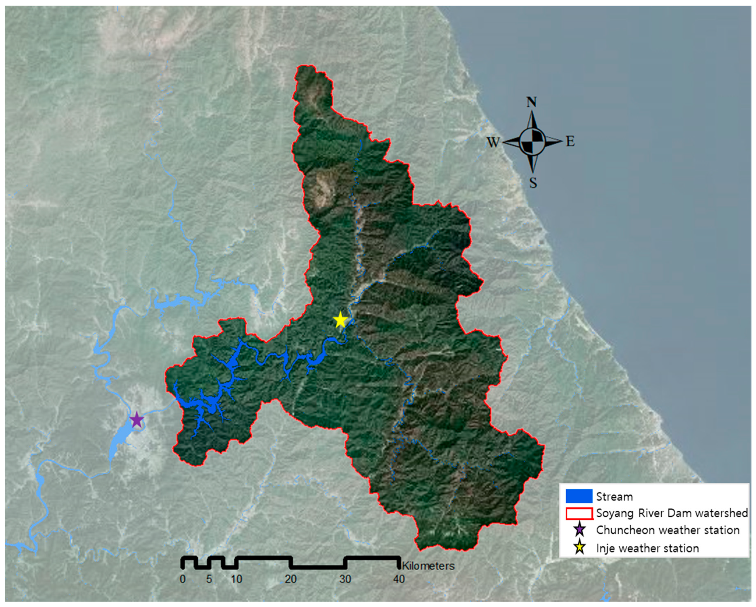
Figure 1. The study area of the Soyang River Dam.
Water 13 03369 g001
Figure 2. Timeseries variation of discharge and inflow of the Soyang River Dam and precipitation data from the Chuncheon weather station and Inje weather station.
Water 13 03369 g002
Figure 3. Illustration of the proposed (a) RNN-LSTM and (d) CNN-LSTM networks for dam discharge prediction.
Water 13 03369 g003
Figure 4. A schematic of the study methodology. Note: The ‘inflow’, ‘discharge’, ‘precip(CC)’, ‘precip(IJ)’, ‘(d−2)’, ‘(d−1)’, and ‘d’ are dam inflow, dam discharge, precipitation at Chuncheon weather station, precipitation at Inje weather station, 2 days ago, 1 day ago, and the day, respectively.
Water 13 03369 g004
Figure 5. Heatmap analysis.
Water 13 03369 g005
Figure 6. The comparisons of forecasting results using machine learning: (a) decision tree, (b) multilayer perceptron, (c) random forest, (d) gradient boosting, (e) LSTM, and (f) CNN-LSTM.
Water 13 03369 g006
Table 1. The input data for machine learning models.
Input VariableOutput Variable
Precipitation and dam data of 2 days agoinflow(d−2), discharge(d−2), precip(CC)(d−2), precip(IJ)(d − 2)Discharge of the day(d)
Precipitation and dam data of 1 day agoinflow(d−1), discharge(d−1), precip(CC)(d−1), precip(IJ)(d−1)
Precipitation and dam data of the day
(forecasted)
Precip(CC)(d), precip(IJ)(d)
Note: The ‘inflow’, ‘discharge’, ‘precip(CC)’, ‘precip(IJ)’, ‘(d−2)’, ‘(d−1)’, and ‘d’ are dam inflow, dam discharge, precipitation at Chuncheon weather station, precipitation at Inje weather station, 2 days ago, 1 day ago, and the day, respectively.
Table 2. The description of machine learning models.
Machine Learning ModelsModuleFunctionNotation
Decision treesklearn.treeDecisionTreeRegressorDT
Multilayer perceptronsklearn.neural_networkMLPRegressorMLP
Random forestsklearn.ensembleRandomForestRegressorRF
Gradient boostingsklearn.ensembleGradientBoostingRegressorGB
RNN-LSTMkeras.models.SequentialLSTM, Dense, DropoutLSTM
CNN-LSTMkeras.models.SequentialLSTM, Dense, Dropout, Conv1D, MaxPooling1DCNN-LSTM
Decision tree, multilayer perceptron, random forest, and gradient boosting used regression functions in the scikit-learn library of Python, whereas RNN-LSTM and CNN-LSTM used sequential functions of Keras modules in the TensorFlow library. ‘Notation’ denotes the abbreviations cited in the figures.
Table 3. The critical hyperparameters in nonlinear regression machine learning algorithms.
Decision Tree RegressorMLP Regressor
HyperparameterValueHyperparameterValue
Criterion
min_samples_leaf
min_impurity_decrease
Splitter
min_samples_split
random_state
Entropy
1
0
best
2
0
hidden_layer_sizes
solver
learning_rate_init
max_iter
momentum
beta_1
epsilon
activation
(50, 50, 50)
adam
0.001
200
0.9
0.9
1× 10⁻⁸
relu
Random Forest RegressorGradient Boosting Regressor
HyperparameterValueHyperparameterValue
n_estimators
min_samples_split
min_weight_fraction_leaf
min_impurity_decrease
verbose
criterion
min_samples_leaf
max_features
bootstrap
52
2
0
0
0
mse
1
Auto
True
Loss
n_estimators
criterion
min_samples_leaf
max_depth
alpha
presort
tol
learning_rate
subsample
min_samples_split
validation_fraction
ls
100
friedman_mse
1
10
0.9
Auto
1 × 10⁻⁴
0.1
1.0
2
0.1
Table 4. Prediction accuracy results of six machine learning models.
MethodNSERMSE
(m3/s)
MAE
(m3/s)
RR2
Decision Tree−0.609137.57818.1030.5300.281
MLP0.48078.20214.2480.7840.614
Random Forest0.76552.55811.0960.8750.765
Gradient Boosting0.31789.60113.0050.7000.490
LSTM0.79648.99610.0240.8980.807
CNN-LSTM0.22195.73013.3720.6550.428
Publisher’s Note: MDPI stays neutral with regard to jurisdictional claims in published maps and institutional affiliations.