Deep Learning in Water Resources Management: Τhe Case Study of Kastoria Lake in Greece

Abstract

The effects of climate change on water resources management have drawn worldwide attention. Water quality predictions that are both reliable and precise are critical for an effective water resources management. Although nonlinear biological and chemical processes occurring in a lake make prediction complex, advanced techniques are needed to develop reliable models and effective management systems. Artificial intelligence (AI) is one of the most recent methods for modeling complex structures. The applications of machine learning (ML), as a part of AI, in hydrology and water resources management have been increasing in recent years. In this paper, the ability of deep neural networks (DNNs) to predict the quality parameter of dissolved oxygen (DO), in Lake Kastoria, Greece, is tested. The available dataset from 11 November 2015, to 15 March 2018, on an hourly basis, from four telemetric stations located in the study area consists of (1) Chl-a (μg/L), (2) pH, (3) temperature—Tw (°C), (4) conductivity (μS/cm), (5) turbidity (NTU), (6) ammonia (NH₄, mg/L), (7) nitrate nitrogen (N–NO₃, mg/L), and (8) dissolved oxygen (DO) (mg/L). Feed-forward deep neural networks (FF-DNNs) of DO, with different structures, are tested for all stations. All the well-trained DNNs give satisfactory results. The optimal selected FF-DNNs of DO for each station with a high efficiency (NSE > 0.89 for optimal selected structures/station) constitute a good choice for modeling dissolved oxygen. Moreover, they provide information in real time and comprise a powerful decision support system (DSS) for preventing accidental and emergency conditions that may arise from both natural and anthropogenic hazards.

1. Introduction

The physical, chemical, and biological responses of lakes to the climate give a variety of priceless information [1]. Lakes are affected directly by changes in climate: (a) due to changes in mixing regime, including lake stratification, oxygen saturation by increase in temperature, and the frequency of extreme wind events; (b) by changes in trophic structure determined by temperature; and (c) by complex interactions between temperature, nutrients, and physical forces [2]. In recent years, waterbodies have undergone extensive change as a result of widespread qualitative and quantitative degradation.

Dissolved oxygen is a very important water quality parameter, and its variation can be wide-ranging over a period of 24 hours [3]. When high concentrations of DO are observed, they mainly occur: (a) at shallow eutrophic lake systems; (b) at late spring–early summer; (c) in the morning and at noon, when high concentrations of DO are observed due to the photosynthetic productivity of algae and/or cyanobacteria, which are also associated with correspondingly high concentrations of Chl-a; and (d) when they are associated with low values of water temperature, which favors high values of DO of saturation, except in cases that the lake has an ice cap, which favors DO consumption and the inability to replenish.

A typical example is the lake of Kastoria, where measured values of DO, higher than those of oxygen saturation (DOs), have been recorded during the spring, mainly in May and June. Therefore, due to the intense activity of the photosynthesis from phytoplankton, from all primary producers of the system, high DO values are observed, which are also associated with correspondingly high concentrations of Chl-a. This phenomenon is reverses in the autumn, when respiration favors photosynthesis and DO depletion occurs, causing stress to the biota [4].

Moreover, when low concentrations of DO are observed, they mainly occur (a) in the evening and night, when no photosynthetic activities take place and the DO is consumed for the respiration of micro-organisms and the degradation of non-preservatives; and (b) at water depths near the bed, where DO values are expected to be very low and may approach hypoxic conditions (1–2 mg/L) or even anoxic conditions (~0 mg/L). Anoxia may also enhance phosphorus release from the sediment into the water column, resulting in increased eutrophic conditions.

Apart from the above reasons, low DO values may occur due to the sediment’s oxygen demand at the bed of a lake, known as sediment oxygen demand (SOD). These low DO values can harm aquatic life, leading to stress, and affect water quality. For this reason, it is necessary to have intensive measurements with many repetitions on a daily basis, so that one can monitor the evolution and the duration of such a phenomenon. During summer, before the advanced phase of eutrophication, where the consumption of DO, due to the respiration activities of benthic biota and invertebrates, is higher than the production of DO, due to photosynthetic activities, concentrations of DO values vary widely [5].

Artificial neural networks (ANNs) are divided into traditional ANNs and deep ANNs and are typically used for both regression and classification problems. ANNs are usually organized into layers, where the learning procedure takes place. The layers consist of a number of units or nodes that are interconnected in such way that one unit is linked to many other units of the same or another layer. The units influence other units by stimulating or inhibiting their activation. To achieve this, the unit receives the weighted sum of all inputs through the links leading to it and produces a single output through the transition function if the sum exceeds a threshold value. The inputs are presented to the network via the input layer that communicates with one or more hidden layers. The hidden layers are associated with the output layer, from where the prediction is given. Deep ANNs are most widely referred to as deep learning (DL) or deep neural networks (DNNs) [6,7].

The concern of scientists, in the applications of artificial neural networks (ANN) in hydrology and water resources management, has been increasing in recent years. The application of artificial neural networks (traditional or deep) has been introduced in the field of hydrological studies and water balance parameters, linear and nonlinear, such as precipitation, evaporation, runoff, and various water quality parameters and it has been concluded that the results produced are quite satisfactory in that concerns the field of forecasting [8,9,10,11,12]. In a developing world, where water is extensively polluted, many models have been applied to predict water quality parameters with the help of machine learning. Artificial machine learning (ANNs), which mimic human brains, are able to map the nonlinear relationships among variables that are characteristic of ecosystems [13]. That is the reason why artificial neural network techniques have been applied in many case studies [14,15] to predict water quality parameters such as dissolved oxygen [16,17,18,19,20]. Nowadays, specifically deep neural networks, as an upgraded and complex version of deep neural networks, have dramatically improved the state-of-the-art in many scientific fields such as environmental studies.

French et al. [21] were first applied a feed-forward ANN to make predictions of abundance of species of phytoplankton in Saidenbach Reservoir in Germany. Cho et al. [22] and Karul et al. [23] used a feed-forward neural network with the help of Levenberg–Marquardt algorithm in order to predict the eutrophication process.

Lek and Guean [24] introduced two kinds of ANNs (back-propagation and Kohonen self-organizing network) in ecology. Yabunaka et al. [25] also applied a back-propagation artificial neural network model to predict algal bloom by simulating the future growth of five phytoplankton species and the Chlorophyll-a (Chl-a) concentrations. In addition, a feed-forward back-propagation artificial neural network model, including one hidden layer, was built by Lu et al. [26] to predict the total phosphorus (TP) concentration in the Lake Champlain.

Zhang et al. [11] applied a multilayer neural network to approach complex regression functions and predict the trends in dissolved oxygen. The aforementioned model gave accurate and better results in predicting the trend of DO than the typical ANN model, support vector regression (SVR) and linear regression model (LRM). Moreover, Kuo et al. [20] gave useful information for effective water quality management by predicting concentrations of water quality and eutrophication problems in the Te-Chi Reservoir in Taiwan by developing a DO back-propagation neural network model. The correlation coefficient between predicted values and measured data was well above 0.7.

In this paper, the ability of deep neural networks to predict the quality parameter of dissolved oxygen, in Lake Kastoria in Greece, is tested. Increases in water temperature lead to reduced oxygen solubility, thus reducing DO concentrations that will have an impact on the duration and intensity of algal blooms [27]. Moreover, the variation of parameters such as DO can be wide-ranging over a period of 24 hours. That is why it is so crucial to have continuous and uninterrupted measurements of the DO concentrations of a lake. The objectives of this paper are (a) to provide a useful supportive tool for water quality management of lakes and (b) to provide real-time prediction of DO in accidental and emergency situations.

The importance of this work lies in the fact that there is no other published work using the same platforms, tools, and methodology of deep learning, as in the present paper, to investigate the predictive capacity of water quality parameters of lakes in real time. Moreover, the fact that Lake Kastoria is monitored by our telemetric stations, offering continuous and uninterrupted data sets (a few hundred thousand), supports the use of deep neural networks, which need large amount of data to complete their learning process, and enhances the originality of the present study.

2. Materials and Methods

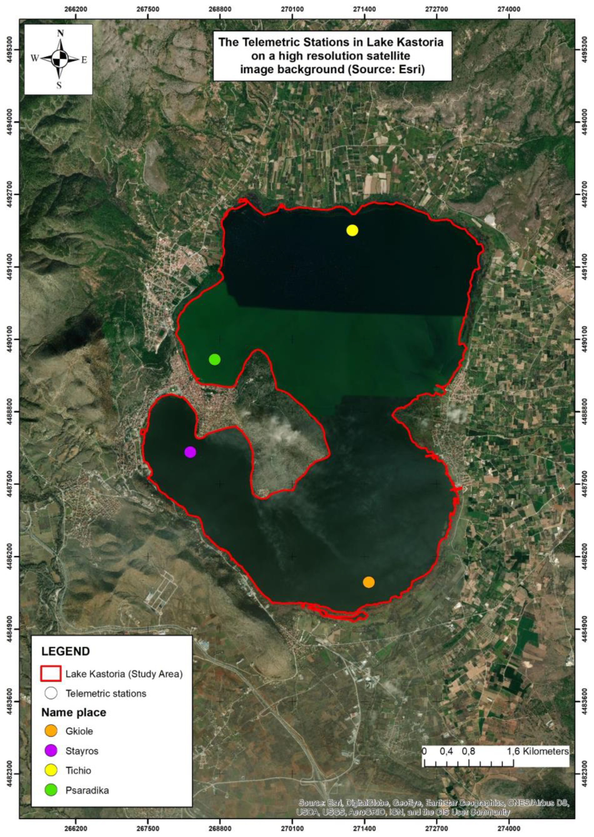
2.1. Study Area

The study area (Figure 1) comprises the catchment area of Lake Kastoria, which is located in the region of Western Macedonia in Greece, protected by directives, regulations, and international conventions. Lake Kastoria is a shallow polymictic lake with intense agricultural activities in its catchment area, which load both point and nonpoint source pollutants. To record water quality characteristics (on the lake’s surface), on an hourly basis, four telemetric stations were installed at specific locations in Lake Kastoria, namely, Gkiole, Stavros, Psaradika, and Toichio.

The aforementioned telemetric stations assist the main monitoring station of Lake Kastoria (according to Directive 2000/60, Law 3199/2003 and JM 140384/2011), both spatially (more stations in different locations) and chronologically (continuous monitoring). After all, without the present monitoring system of Lake Kastoria, it would be impossible to apply deep neural network techniques.

The criteria of the choice of the monitoring stations in the present positions were: (a) the environmental pressures occurring from the land uses of the catchment area; (b) the hydromorphological characteristics of the lake; (c) the presence of corrosion, transport, and deposition phenomena; (d) the inflows and outflows; and (f) issues related to the accessibility and the costs of stations’ installation and maintenance.

2.2. Programming Language

The Python programming language is used for the purpose of the study. Its main feature is its flexibility, as the same piece of code can be used with little or no change over a wide range of devices with different architectural and computing capabilities [28]. Another advantage is the use and interconnection of many libraries, which makes it an ideal programming language for developing ML models that use many different libraries and platforms. One of its applications is to develop DNNs.

2.3. Tools and Platforms

To develop DNNs—based on machine learning methods—the Python programming language, the Spyder scientific environment, the Tensorflow open-source machine learning platform, and Nvidia’s Compute Unified Device Architecture (CUDA) parallel platform (graphics card) are used. All of the above have been integrated into Anaconda, an open-source programming language. The CUDA platform is a parallel computing platform developed by Nvidia that enables users to exploit the computing power of graphics card kernels for training and testing machine learning models. This results in the verification and creation of many models very fast. The main reason for using Anaconda and CUDA is that the model can be created in a variety of virtual environments and with the possibility of using parallel programming through the computing power of the graphics card. The above procedure gives the user the advantage of using large databases, such as in the present study, and complex learning algorithms, without having to install and reinstall various versions of libraries, offering training, verification, and testing of the model in a very short time [29].

2.4. Graphical User Interface

The Spyder scientific environment, written in Python, is used as it offers a unique combination of the advanced editing, analysis, debugging, and profiling functionality with an integrated deployment tool with interactive execution, data exploration, and visualization capabilities of a scientific package. Spyder is also an open-source code-processing environment, but only for the Python programming language. The Spyder environment enables the user to execute code line by line while displaying the results for each execution step. This allows the user to see if each step of the code is able to print individual diagrams or sections of code without having to re-execute the entire code again [30].

2.5. Libraries

Various libraries (Pathlib, Matplotlib, Pandas, Seaborn) have been used for Python programming. The libraries needed are not loaded in default. For that reason, a good practice to begin the code is by importing all the libraries needed. The most important of all libraries is the open-source Tensorflow machine learning library. The Tensorflow platform is an end-to-end open-source platform for developing machine learning models, developed by Google. It consists of a comprehensive, flexible ecosystem set of tools and libraries that allow users to easily use and develop ML models [31]. This library provides state-of-the-art machine learning methods, allowing the users to create their own machine learning models in a user-friendly, multipack, and add-on environment. In the present study, the Tensorflow GPU library is used, which enables the user with the CUDA tool to train and test the models they have developed through the computing power of the graphics card kernels.

2.6. Input and Output Data

The predictive ability of networks is based on their training, which in turn depends on the amount of information available on the network. For the purpose of this study, time series of quality parameters from 11 November 2015 to 15 March of 2018 were used on an hourly basis from four telemetric stations located in the study area, namely, Gkiole, Toichio, Psaradika, and Stavros (

Table 1. Number of data/parameter.

Station	Number of Data/Parameter
Gkiole	16,922
Toichio	19,763
Psaradika	16,574
Stavros	19,154

). More specifically, the available data consist of (1) Chl-a (µg/L), (2) pH, (3) Tw (°C), (4) ECw (μS/cm), (5) turbidity (NTU), (6) ammonia nitrogen (N–NH₄, ppm) (not available (NA) data for Stavros station), (7) nitrate nitrogen (N–NO₃, mg/L), and (8) dissolved oxygen (mg/L). Indicatively, the descriptive statistics of the available data are given for Toichio station (

Table 2. Descriptive statistics of the water quality data for Toichio Station.

Variables	Unit	Mean	Std Dev	Min	25%	50%	75%	Max
Chlorophyll-a	μg/L	11.74	11.48	0.30	5.40	8.40	14.10	453.30
Conductivity	μS/cm	316.18	25.26	239.00	307.00	318.00	331.00	369.00
pH	-	8.41	0.35	5.40	8.10	8.40	8.60	9.80
Turbidity	NTU	20.87	52.28	0.10	0.00	1.80	49.00	3000.00
Temperature	oC	14.33	7.83	0.80	6.80	13.80	21.80	30.40
NH4	mg/L	0.56	1.14	0.10	0.00	0.10	0.60	19.70
NO3	mg/L	1.30	0.74	0.01	0.83	1.24	1.70	3.72
DO	mg/L	8.10	2.60	0.01	6.34	8.29	9.73	18.27

).

An important step in DL is the selection of appropriate input variables. Based on the literature, neural network studies reported that most important water quality parameters, for the modeling of dissolved oxygen, are pH and water temperature [15,19]. In addition to those two inputs, the importance of NO₃–N and NH₄–N as input variables for DO models has been proposed [19,20]. Moreover, turbidity [13], Chl-a [20], and ECw [17,19] have been reported as input variables for DO modeling. Here, based on the literature [15,17,19,20], all the available parameters are taken into account as input parameters for each investigated model. Subsequently, based on the literature and taking into account the resulting tables, concerning the impact of each input parameter to the output parameter (DO), DNNs consisting of four input parameters, namely, (1) nitrate nitrogen (N–NO₃, mg/L), (2) pH, (3) Tw (°C), and (4) ECw (μS/cm), are also tested.

2.7. Number of Hidden Layers

The generalization capability of a neural network is linked to its hidden layer. Too many hidden layers in a network increase computational burden and cause over-fitting, which results in poor prediction. Several studies [32,33] show that one or two hidden layers mostly produce better performance. It should be reminded that if an ANN has more than three layers, including input and output layers, it is called a deep neural network [34]. As the scope of this paper is to apply a deep neural network for modeling and prediction of quality parameter, two hidden layers are used for different structures.

2.8. Number of Nodes in the Hidden Layer

Deciding the appropriate number of nodes is crucial for effective learning and performance of the network. Nevertheless, there is no systematic approach to determine the optimal number of nodes to utilize for a problem [32,33]. Here, a preliminary investigation of deep neural networks for simulation and real-time prediction is used as default 64 neurons per hidden layer. The predictive ability of a deep neural network, consisting of 32 nodes per hidden layer, is also tested.

2.9. Training Epochs

In order to train a neural network, many epochs (cycles of training process) are needed. Some studies [32,33] have indicated that convergence could be achieved by training 85 to 5000 epochs. Here, 1000 epochs were able to achieve the convergence.

2.10. Activation Function

Activation functions are an essential part of neural networks as they provide nonlinearity. The absence of nonlinearity turns the neural network to a simple logistic regression model. Here, the rectified linear unit (ReLU) is used, which is defined as (Equation (1)):

f(x) = max (0, x)

(1)

where x is the input to the neuron.

An advantage of ReLU is that it is a highly simplified and easy-to-calculate function. It is also very quick to use and train compared with other activation functions. Moreover, in ML, updating a parameter is proportional to the partial derivative of the error function with respect to these parameters. If the gradient becomes too small, the updates will not work and the network may stop the training procedure. ReLU does not saturate in the positive direction, while other activation functions such as sigmoid and hyperbolic tangent saturate in both directions. Therefore, it has fewer vanishing gradients, resulting in better training. The limitation of ReLU is that its mean output is not zero [35].

2.11. Learning Rate

The learning rate is a hyper-parameter that controls how much to change the model in response to the estimated error each time the model weights are updated. If the learning rate is too large, the network fails to converge with allowable error over training set. Choosing a too small learning rate results in slow training process. Most of the neural networks utilize a value from 0.01 to 0.3 of the learning rate. In the present paper, taking advantage of the computing power of the graphic card, a learning rate of 0.001 is used.

2.12. Optimization Algorithm

With a strong ability to find the most optimistic result, RMSprop is used. RMSprop is one of the most popular optimization algorithms used in DL, as it is a fast and good optimizer [30]. It uses a moving average of squared gradients to normalize the gradient itself. It has an effect of balancing the step size; it decreases the step for a large gradient to avoid exploding and increases the step for a small gradient to avoid vanishing. RMSprop avoids the decay of the learning rate to zero.

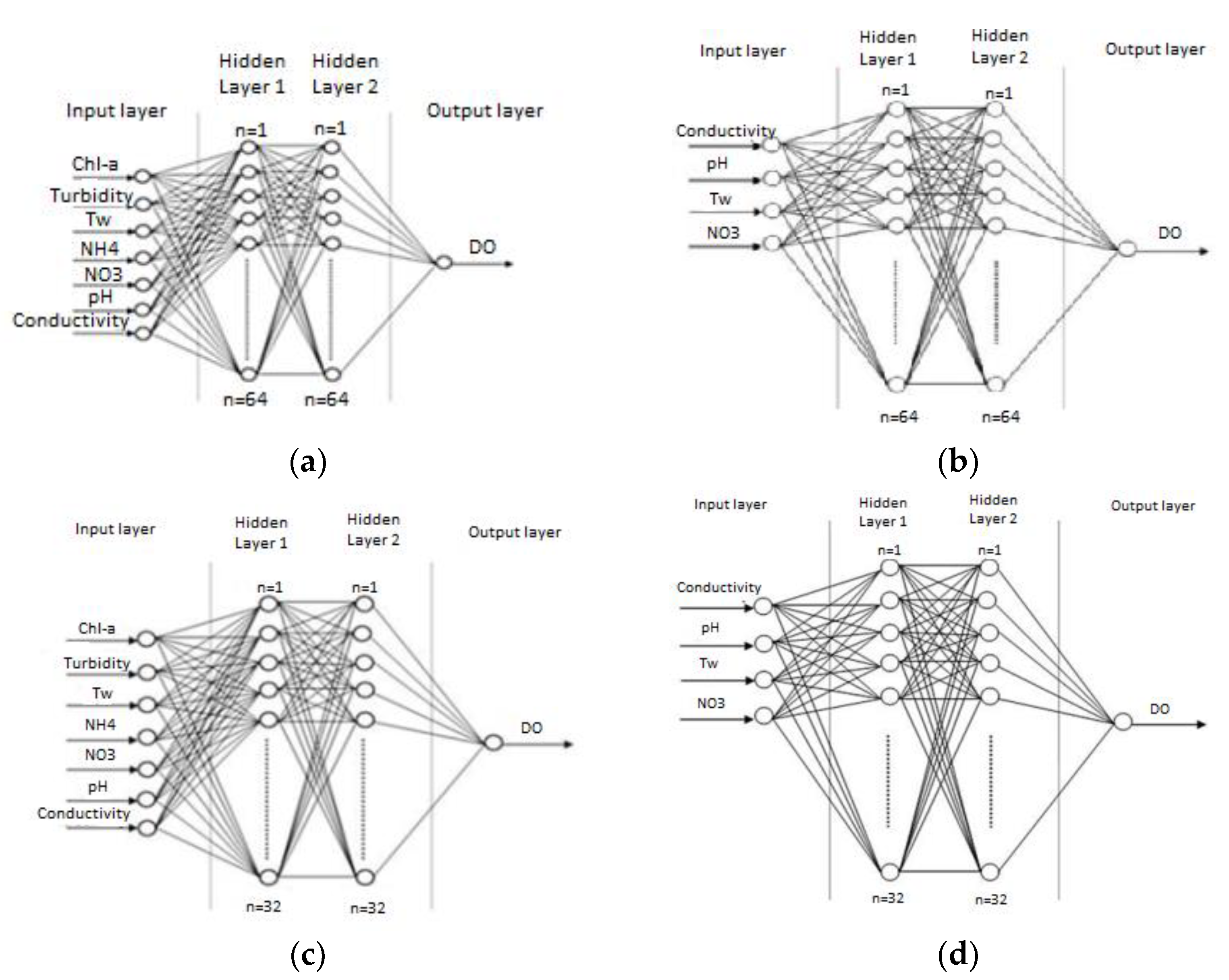
2.13. The Structures

Deep learning-based technique is used in order to develop the DO model, which is applied to the data of the four stations separately. To achieve the goal, a DNN was built for each case consisting of:

• an input layer of quality parameters, depending on the investigated structure;
• two densely connected hidden layers, consisting of 64 or 32 units/nodes each, depending on the investigated structure; and
• an output layer of DO quality parameter.

The examined deep neural networks structures are listed below:

The DO model with structures:

• 7-64-64-1 for Gkiole, Psaradika, and Toichio stations (Figure 2a) and 6-64-64-1 for Stavros station, where NH₄ parameter is not available;
• 4-64-64-1 for all stations (Figure 2b);
• 7-32-32-1 for Gkiole, Psaradika, and Toichio stations (Figure 2c) and 6-32-32-1 for Stavros station where NH₄ parameter is not available; and
• 4-32-32-1 for all stations (Figure 2d).

Here, a DNN with structure, for example, 7-64-64-1, indicates a model comprising 7 inputs, 64 nodes per hidden layer, and 1 output node. In terms of how the nodes are connected to each other, a feed-forward neural network is used for each case, as there is no feedback from the outputs toward the inputs.

2.14. Preparation of the Dataset

In this context, there were three phases—training, testing, and validation—for each station. In total, 80% of the data was used for the training process and 20% for testing, and 80% of the training data was re-divided into 60% for the training process and the remaining 20% for validation.

2.15. Statistical Descriptors

The following statistical measures were used to evaluate the predictive ability of the neural network models: (a) the mean absolute error (MAE), (b) the mean square error (MSE), and (c) the Nash–Sutcliffe model efficiency coefficient (NSE).

3. Results

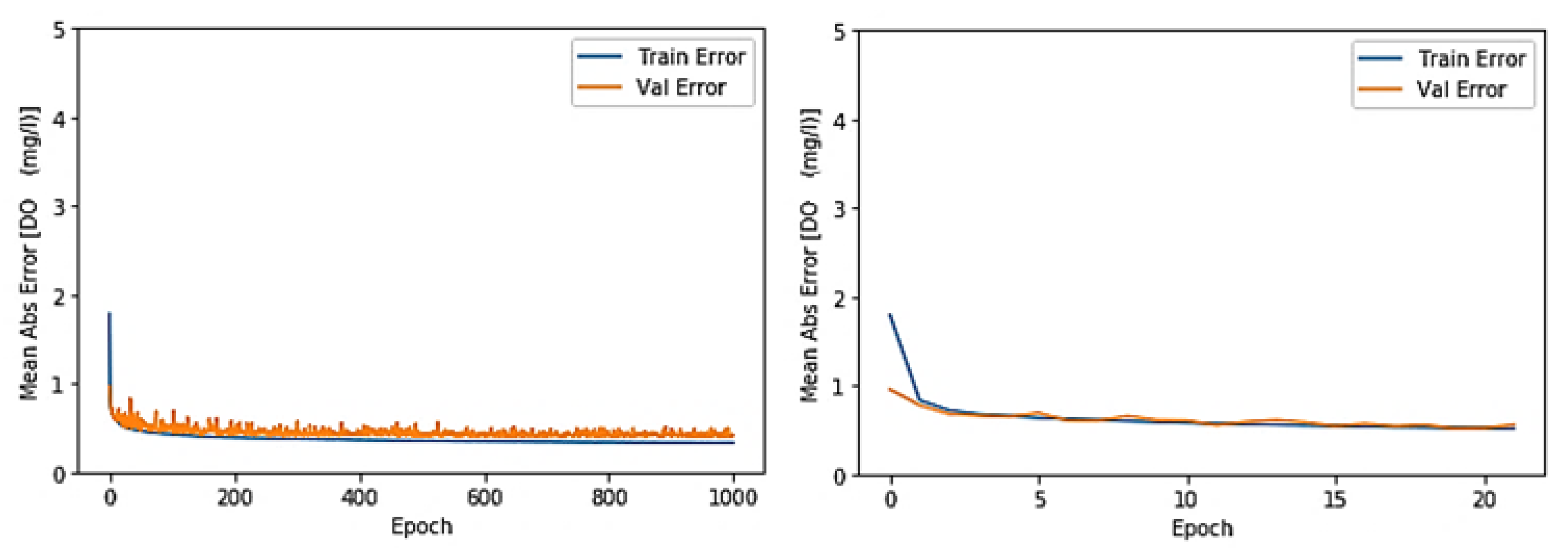
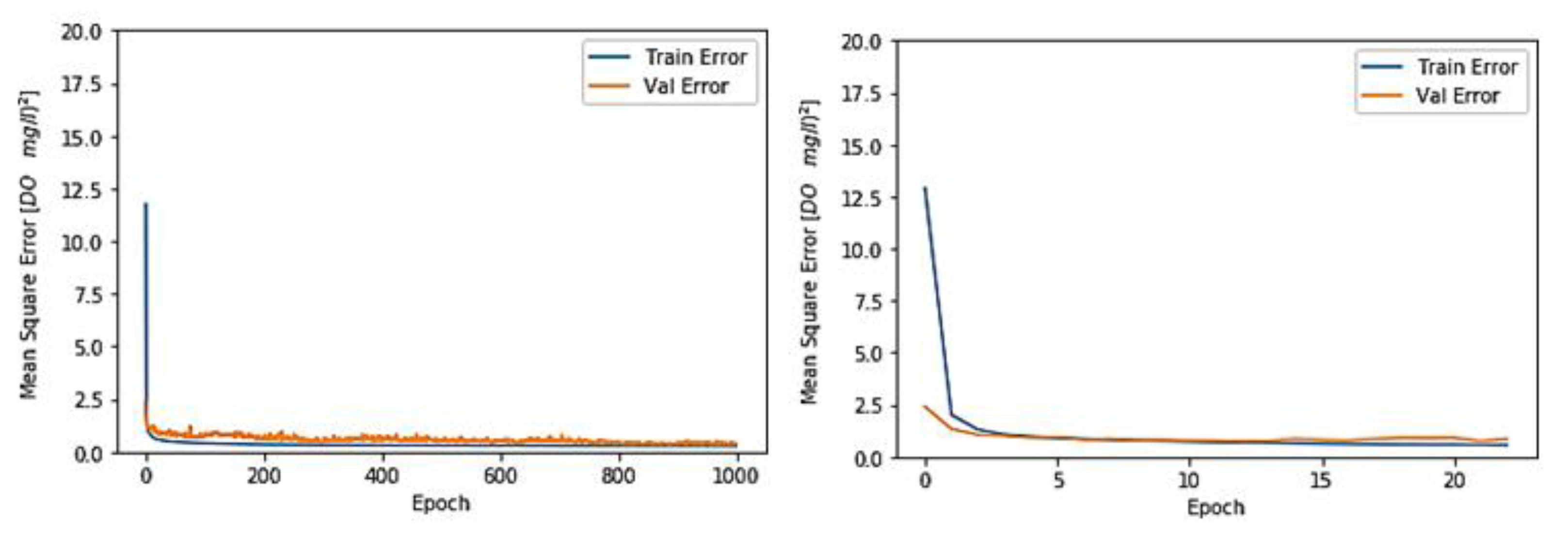
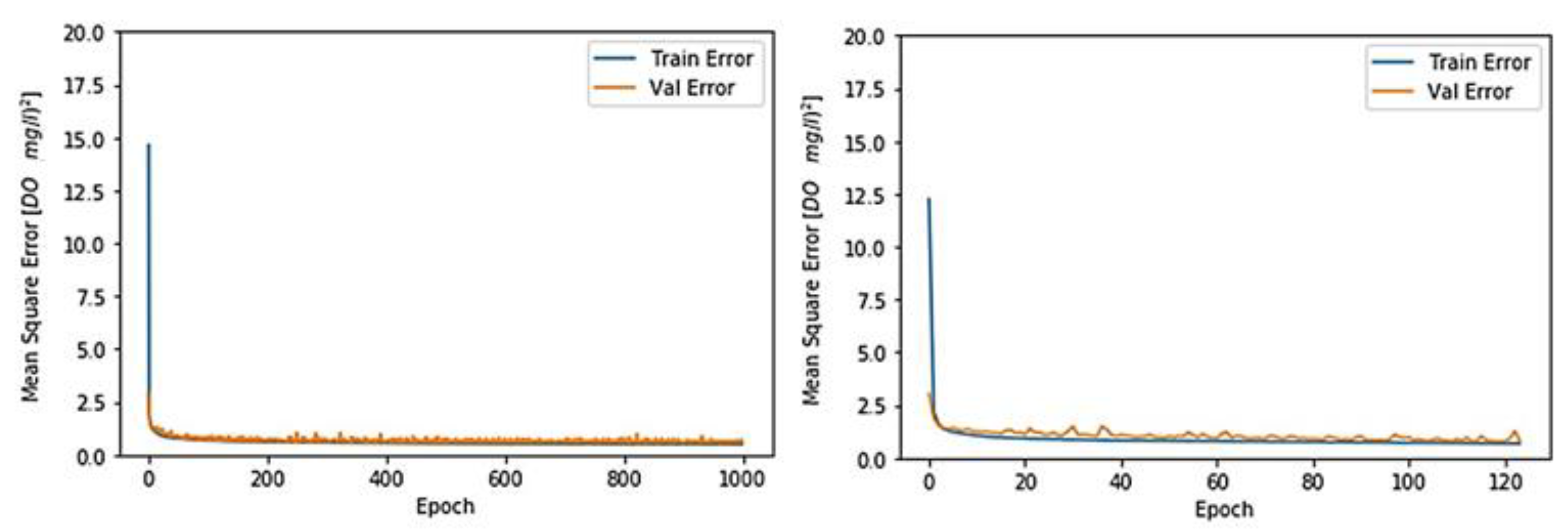
3.1. Toichio Station

The procedure that was followed is described in detail for Toichio station. The same procedure was followed for all the examined stations and structures, the results of which are given in

Table 3. Statistical descriptors of the investigated structures for all stations.

Station	Structure	Training			Test
		MAE	MSE	NSE	MAE	MSE	NSE
Gkiole	7-64-64-1	0.69	0.89	0.81	0.71	0.92	0.79
	4-64-64-1	0.58	0.83	0.84	0.61	0.85	0.82
	7-32-32-1	0.54	0.65	0.89	0.55	0.68	0.86
	4-32-32-1	0.64	0.84	0.82	0.67	0.94	0.81
Toichio	7-64-64-1	0.48	0.52	0.92	0.49	0.51	0.93
	4-64-64-1	0.62	0.70	0.89	0.62	0.72	0.91
	7-32-32-1	0.50	0.54	0.91	0.54	0.57	0.92
	4-32-32-1	0.58	0.76	0.90	0.62	0.77	0.91
Psaradika	7-64-64-1	0.60	0.77	0.88	0.63	0.80	0.90
	4-64-64-1	0.57	0.65	0.91	0.58	0.68	0.92
	7-32-32-1	0.57	0.70	0.89	0.58	0.72	0.90
	4-32-32-1	0.58	0.69	0.89	0.60	0.71	0.90
Stavros	6-64-64-1	0.73	1.02	0.87	0.74	1.08	0.86
	4-64-64-1	0.69	1.07	0.88	0.72	1.11	0.86
	6-32-32-1	0.69	0.98	0.91	0.70	1.01	0.90
	4-32-32-1	0.73	1.23	0.86	0.78	1.30	0.85

.

3.1.1. Structure: 7-64-64-1

Figure 3 and Figure 4 illustrate the mean absolute error and the mean square error of the DO model for Toichio station, respectively, during the training process of 1000 epochs. The model seems to “learn” from the dataset after the 20th epoch. The training means absolute error equals to 0.48, while the training means square error equals to 0.52. Moreover, the resulting values of mean absolute error and mean square error for test set equal to 0.49 and 0.51, respectively. The fact that the obtained training errors were slightly lower than the tested ones indicates that a good fit is obtained. Figure 5 shows that the DO model with structure 7-64-64-1 for Toichio station predicts very well. Finally, Figure 5 illustrates the prediction error distribution.

3.1.2. Structure: 4-64-64-1

Figure 6 and Figure 7 demonstrate the mean absolute error and the mean square error of the DO model, respectively, with structure 4-64-64-1 for Toichio station, during the training process of 1000 epochs. The model “understands” the dataset after the 40th epoch. The training means absolute error equals to 0.62, while the training means square error equals to 0.70. Moreover, the testing means absolute error and mean square error equal to 0.62 and 0.72, respectively, showing that the DO model predicts reasonably well. Finally, Figure 8 illustrates the true values versus the predicted ones and the prediction error distribution.

3.1.3. Structure: 7-32-32-1

The DO model with structure 7-32-32-1 produces results with an MAE of 0.50 and 0.54 and an MSE of 0.54 and 0.57 for the training and the testing process, respectively, for Toichio station. The training process takes place for 1000 epochs, and convergence is achieved (Figure 9 and Figure 10). Finally, Figure 11 shows the prediction error distribution of the DO models for the aforementioned station.

3.1.4. Structure: 4-32-32-1

The dissolved oxygen model with structure 4-32-32-1 produces results with MAE of 0.58 and 0.62 and the MSE of 0.76 and 0.77 for the training and the testing process, respectively, for Toichio station (Figure 12 and Figure 13). Figure 14 shows the obtained versus the predicted values and the prediction error distribution. The DO model with structure 4-32-32-1 predicts reasonably well.

3.2. All Stations/Structure

The dissolved oxygen models are trained for two different numbers of neurons in the hidden layers and for two different input combinations. All the investigated structures give satisfactory results. The optimal network architecture of each structure for each station is selected based on the one with the minimum statistical descriptors of MAE and MSE. The NSE is used to assess the predictive power of the models. The lower the MAE and MSE, the more the model is optimized (NSE reaches the unit). Overall, four structures are compared as shown in Table 3 for each station.

The well-trained DNN with structure 7-32-32-1 produces results with an MAE of 0.54 and 0.55 and an MSE of 0.65 and 0.68 for the training and the testing process, respectively, with a good predictive ability for Gkiole station. For Toichio station, the structure 7-64-64-1 prevails with an MAE of 0.48 and 0.49 and an MSE of 0.52 and 0.51 for the training and the testing process, respectively, and it constitutes the structure with the best performance compared with all the structures for all stations. For Psaradika station, the structure 4-64-64-1 produces the best results in relation to the other structures of this station with an MAE of 0.57 and 0.58 and an MSE of 0.65 and 0.68 for the training and the testing process, respectively. Finally, Stavros station presents results with an MAE of 0.69 and 0.70 and an MSE of 0.98 and 1.01 for the training and the testing process, respectively (structure 6-32-32-1). However, the selected structure 6-32-32-1 for Stavros station is less appropriate compared to the aforementioned selected structures for Gkiole, Toichio, and Psaradika stations.

It should be mentioned that, in all the investigated structures, the training errors are slightly lower than the tested ones, which indicates that a good fit has been achieved. Based on the investigated structures, the results demonstrate that the proposed DNN models (

Table 4. The optimal selected structures for each station.

Station	Structure	Training			Test
		MAE	MSE	NSE	MAE	MSE	NSE
Gkiole	7-32-32-1	0.54	0.65	0.89	0.55	0.68	0.86
Toichio	7-64-64-1	0.48	0.52	0.92	0.49	0.51	0.93
Psaradika	4-64-64-1	0.57	0.65	0.91	0.58	0.68	0.92
Stavros	6-32-32-1	0.69	0.98	0.91	0.70	1.05	0.90

) constitute a good choice for modeling dissolved oxygen for each station. Table 4 also illustrates the high efficiency of the selected structures.

4. Discussion

It is clear that the models that show the most appropriate predictive ability, based on their statistical descriptors for Gkiole, Toichio, and Stavros stations, are the models consisting of all the input parameters. Despite the fact that not all the input parameters have a high impact on the output, the use of all the available information seems to give a better performance in deep learning. In other words, all the parameters have a significant effect on the performance of the DNN model and cannot be excluded from the input variables. This inability to explain network behavior may seem unacceptable to the scientist, but one should remember that when one is moving in the ambiguous contexts of stochastic phenomena and, in particular, artificial intelligence, this may not only be acceptable, but that is the scope. Moreover, the structure and function of the network becomes “autonomous,” achieving the idea of “machine learning”.

In case of Psaradika station, the selected model does not use all the parameters to achieve good performance, but it needs a deep network of 64 nodes per layer instead of 32 in order to give the best results compared to other structures for this station. The fact that the model with structure 4-32-32-1, utilizing fewer inputs and nodes in hidden layers, is less appropriate in relation to all the investigated models for all stations, constitutes the evidence that complex neural networks are a promising field for improvement. The use of the selected tools and platforms gives the advantage of using large databases, while the training and testing procedure is obtained in a very short time (GPU card).

Learning rate is a crucial hyper-parameter in deep learning, controlling how much to change the model in response to the estimated error, each time the model weights are updated. If the learning rate is too large, the network fails to converge. Most of the neural networks utilize a value from 0.01 to 0.3 of the learning rate. In the present study, taking advantage of the computing power of the graphic card, a learning rate of 0.001 is used. Moreover, the Tensorflow provides state-of-the-art machine learning methods, and the possibility of using parallel programming through the computing power of the graphics card makes the process of machine learning constantly gain ground.

The optimal selected feed-forward deep neural networks (DNN) of the DO for each station provide information comprising a powerful decision support system (DSS) to prevent accidental and emergency conditions that may arise from both natural and anthropogenic hazards in real time. In practice, the use of neural networks in hydrology tends to mimic hydrological processes, which science does not fully understand or can express with the help of a mathematical formula. However, it should be noted that, according to their structure and function, neural networks generally do not provide a better understanding of hydrological processes and natural phenomena, as they simplify physics and “degenerate” into weights and threshold values. To select the appropriate network structure and to apply the appropriate training algorithm, one must understand the natural procedures that occur. Moreover, the right choice of network architecture, activation functions, and learning methods could be substantiated through a test and control process. In addition, the selection of training data is of paramount importance, as it requires proper preparation and normalization. However, from a water management point of view, due to the user-friendly nature of the proposed neural networks, they can be implemented in real time by nonspecialists, as no knowledge of the phenomenon is required after the end of training phase.

The possible future work could include the following:

• Use additional information captured from a modern drone (uncrewed aerial vehicle) equipped with a multispectral camera as ground-truth information to calibrate satellite imagery in order to improve quantification of the specific quality parameters of the water from the study area. The additional information could also be enhanced by using data (ground data collection) derived from field work (targeted area samplings) in the study area. The existing operational algorithms could be tested, or maybe new ones could be created in order to find the best fit of the band ratio.
• Use more complex machine learning methods (such as convolutional neural networks (CNNs)), not only for Lake Kastoria but also for other national and international lakes, mainly in neighboring countries with cross-border water resources.
• Use the same methodology in order to test the adequacy of the proposed models for other national and international lakes.

5. Conclusions

The selected DO models for each station provide information in real time and comprise a powerful decision support system (DSS) for preventing accidental and emergency conditions. The real-time monitoring of the water quality parameters contributes in management by (a) controlling water quality for irrigation, (b) monitoring atmospheric conditions, (c) determining microclimate indicators, (d) issuing a warning in case of crises caused by extreme events, (e) providing continuous knowledge of the state of the water bodies, and (f) maintaining the ecological balance of the ecosystems and water resources of the region.

References

1. Williamson, C.E.; Saros, J.E.; Vincent, W.F.; Smol, J.P. Lakes and reservoirs as sentinels, integrators, and regulators of climate change. Limnol. Oceanogr. 2009, 54, 2273–2282. [Google Scholar] [CrossRef]
2. Jeppesen, E.; Kronvang, B.; Meerhoff, M.; Søndergaard, M.; Hansen, K.M.; Andersen, H.E.; Lauridsen, T.L.; Liboriussen, L.; Beklioglu, M.; Özen, A.; et al. Climate change effects on runoff, catchment phosphorus loading and lake ecological state, and potential adaptations. J. Environ. Qual. 2009, 38, 1930–1941. [Google Scholar] [CrossRef]
3. Psilovikos, A. The Contribution of Monitoring to the Rational Management and Prevention of Environmental Risks on the Nestos Transboundary River. The perspective for the implementation of Directive 2000/60. Hydrotechnica 2005, l15, 87–102. [Google Scholar]
4. Mantzafleri, N.; Psilovikos, A.; Mplanta, A. Water quality monitoring and modeling in Lake Kastoria, using GIS. Assessment and management of pollution sources. Water Resour. Manag. 2009, 23, 3221–3254. [Google Scholar] [CrossRef]
5. Sammut, C.; Webb, G.I. Encyclopedia of Machine Learning and Data Mining; Springer Publishing Company: Berlin/Heidelberg, Germany, 2017; Volume 32. [Google Scholar]
6. Liakos, K.G.; Busato, P.; Moshou, D.; Pearson, S.; Bochtis, D. Machine Learning in agriculture: A review. Sensors 2018, 18, 2674. [Google Scholar] [CrossRef] [PubMed] [Green Version]
7. Diamantopoulou, M.J.; Papamichail, D.M.; Antonopoulos, V.Z. The use of a Neural Network technique for the prediction of Water Quality parameters. Oper. Res. 2005, 5, 115–125. [Google Scholar] [CrossRef]
8. Alizadeh, M.J.; Kavianpour, M.R. Development of wavelet-ANN models to predict water quality parameters in Hilo Bay, Pacific Ocean. Mar. Pollut. Bull. 2015, 98, 171–178. [Google Scholar] [CrossRef] [PubMed]
9. Karamoutsou, L.; Psilovikos, A. The Use of Artificial Neural Networks in Predicting the Water Quality of Lake Kastoria. In Proceedings of the 14th Conference of the Hellenic Hydrotechnical Association (EYE), Volos, Greece, 16–17 May 2019. [Google Scholar]
10. Sentas, A.; Karamoutsou, L.; Charizopoulos, N.; Psilovikos, T.; Psilovikos, A.; Loukas, A. The use of Stochastic Models for short term predictions of Water Parameters of the Thesaurus Dam, Nestos River, Greece. In Proceedings of the 3rd EWaS International Conference, Lefkada, Greece, 27–30 June 2018. [Google Scholar]
11. Zhang, Y.; Fitch, P.; Thorburn, P.; Vilas, M.D.L.P. Applying multi-layer artificial neural network and mutual information to the prediction of trends in dissolved oxygen. Front. Environ. Sci. 2019, 7, 46. [Google Scholar] [CrossRef]
12. Lek, S.; Delacoste, M.; Baran, P.; Dimopoulos, I.; Lauga, J.; Aulagnier, S. Application of Neural Networks to modelling nonlinear relationships in ecology. Ecol. Model. 1996, 90, 36–52. [Google Scholar] [CrossRef]
13. Chen, J.; Wang, Y. Comparing Activation Functions in Modeling Shoreline Variation Using Multilayer Perceptron Neural Network. Water 2020, 12, 1281. [Google Scholar] [CrossRef]
14. Mellios, N.; Moe, S.; Laspidou, C. Machine Learning Approaches for Predicting Health Risk of Cyanobacterial Blooms in Northern European Lakes. Water 2020, 12, 1191. [Google Scholar] [CrossRef] [Green Version]
15. Ranković, V.; Radulović, J.; Radojević, I.; Ostojić, A.; Čomić, L. Neural network modeling of dissolved oxygen in the Gruža reservoir, Serbia. Ecol. Model. 2010, 221, 1239–1244. [Google Scholar] [CrossRef]
16. Akkoyunlu, A.; Altun, H.; Cigizoglu, H.K. Depth-integrated estimation of Dissolved Oxygen in a lake. J. Environ. Eng. 2011, 137, 961–967. [Google Scholar] [CrossRef]
17. Ay, M.; Kisi, O. Modeling of dissolved oxygen concentration using different neural network techniques in Foundation Creek, El Paso County, Colorado. J. Environ. Eng. 2012, 138, 654–662. [Google Scholar] [CrossRef]
18. Han, H.G.; Qiao, J.F.; Chen, Q.L. Model predictive control of dissolved oxygen concentration based on a self-organizing RBF neural network. Control Eng. Pract. 2012, 20, 465–476. [Google Scholar] [CrossRef]
19. Wen, X.; Fang, J.; Diao, M.; Zhang, C. Artificial neural network modeling of dissolved oxygen in the Heihe River, Northwestern China. Environ. Monit. Assess. 2013, 185, 4361–4371. [Google Scholar] [CrossRef] [PubMed]
20. Kuo, J.T.; Hsieh, M.H.; Lung, W.S.; She, N. Using Artificial Neural Network for reservoir eutrophication prediction. Ecol. Model. 2007, 200, 171–177. [Google Scholar] [CrossRef]
21. French, M.; Recknagel, F. Modeling algal blooms in freshwaters using artificial neural networks. In Computer Techniques in Environmental Studies V, Vol. II: Environment Systems; Zanetti, P., Ed.; Computational Mechanics Publications: Boston, MA, USA, 1994; pp. 87–94. [Google Scholar]
22. Cho, S.; Lim, B.; Jung, J.; Kim, S.; Chae, H.; Park, J.; Park, S.; Park, J.K. Factors affecting algal blooms in a man-made lake and prediction using an Artificial Neural Network. Measurement 2014, 53, 224–233. [Google Scholar] [CrossRef]
23. Karul, C.; Soyupak, S.; Cilesiz, A.F.; Akbay, N.; Germen, E. Case studies on the use of neural networks in eutrophication modelling. Ecol. Model. 2000, 134, 145–152. [Google Scholar] [CrossRef]
24. Lek, S.; Guean, J.F. Artificial Neural Networks as a tool in ecological modeling, an introduction. Ecol. Model. 1999, 120, 65–73. [Google Scholar] [CrossRef]
25. Yabunaka, K.-I.; Hosomi, M.; Murakami, A. Novel application of a backpropagation artificial neural network model formulated to predict algal bloom. Water Sci. Technol. 1997, 36, 89–97. [Google Scholar] [CrossRef]
26. Lu, F.; Zhang, H.; Liu, W. Development and application of a GIS-based artificial neural network system for water quality prediction: A case study at the Lake Champlain area. J. Oceanol. Limnol. 2020, 38, 1835–1845. [Google Scholar] [CrossRef]
27. Hosseini, N.; Johnston, J.; Lindenschmidt, K.E. Impacts of climate change on the water quality of a regulated prairie river. Water 2017, 9, 199. [Google Scholar] [CrossRef] [Green Version]
28. Abadi, M.; Barham, P.; Chen, J.; Chen, Z.; Davis, A.; Dean, J.; Devin, M.; Ghemawat, S.; Irving, G.; Isard, M.; et al. Tensorflow: A system for large-scale machine learning. In Proceedings of the 12th (USENIX) Symposium on Operating Systems Design and Implementation, Savannah, GA, USA, 2–4 November 2016. [Google Scholar]
29. Deep Learning. Available online: https://developer.nvidia.com/deep-learning (accessed on 15 January 2020).
30. Spyder. The scientific Python Development Environment. Available online: https://www.spyder-ide.org/ (accessed on 15 January 2020).
31. Tensorflow. Available online: https://www.tensorflow.org/overview (accessed on 15 January 2020).
32. Smithson, S.C.; Yang, G.; Gross, W.J.; Meyer, B.H. Neural networks designing neural networks: Multi-objective hyper-parameter optimization. In Proceedings of the 35th International Conference on Computer-Aided Design, Austin, TX, USA, 7–10 November 2016. [Google Scholar]
33. Gaya, M.S.; Zango, M.U.; Yusuf, L.A.; Mustapha, M.; Muhammad, B.; Sani, A.; Tijjani, A.; Wahab, N.A.; Khairi, M.T.M. Estimation of turbidity in water treatment plant using Hammerstein-Wiener and neural network technique. Indones. J. Electr. Eng. Comput. Sci. 2017, 5, 666–672. [Google Scholar] [CrossRef]
34. Kriegeskorte, N.; Golan, T. Neural network models and deep learning. Curr. Biol. 2019, 29, 231–236. [Google Scholar] [CrossRef] [PubMed]
35. Hossen, T.; Plathottam, S.J.; Angamuthu, R.K.; Ranganathan, P.; Salehfar, H. Short-term load forecasting using deep neural networks (DNN). In Proceedings of the 2017 North American Power Symposium (NAPS), IEEE, Morgantown, WV, USA, 17–19 September 2017. [Google Scholar] [CrossRef]
Figure 1. The position of telemetric stations in Lake Kastoria [9].
Water 13 03364 g001
Figure 2. Different structures of DO models: (a) 7-64-64-1 for Gkiole, Psaradika, and Toichio stations and 6-64-64-1 for Stavros station, where NH4 parameter is not available; (b) 4-64-64-1 for all stations; (c) 7-32-32-1 for Gkiole, Psaradika, and Toichio stations and 6-32-32-1 for Stavros station, where NH4 parameter is not available; (d) 4-32-32-1 for all stations.
Water 13 03364 g002
Figure 3. Mean absolute error (Toichio station, structure 7-64-64-1).
Water 13 03364 g003
Figure 4. Mean square error (Toichio station, structure 7-64-64-1).
Water 13 03364 g004
Figure 5. True vs. predicted values (left); predicted error (right) (Toichio station, structure 7-64-64-1).
Water 13 03364 g005
Figure 6. Mean absolute error (Toichio station, structure 4-64-64-1).
Water 13 03364 g006
Figure 7. Mean square error (Toichio station, structure 4-64-64-1).
Water 13 03364 g007
Figure 8. True vs. predicted values (left); predicted error (right) (Toichio station, structure 4-64-64-1).
Water 13 03364 g008
Figure 9. Mean absolute error (Toichio station, structure 7-32-32-1).
Water 13 03364 g009
Figure 10. Mean square error (Toichio station, structure 7-32-32-1).
Water 13 03364 g010
Figure 11. True vs. predicted values (left); predicted error (right) (Toichio station, structure 7-32-32-1).
Water 13 03364 g011
Figure 12. Mean absolute error (Toichio station, structure 4-32-32-1).
Water 13 03364 g012
Figure 13. Mean square error (Toichio station, structure 4-32-32-1).
Water 13 03364 g013
Figure 14. True vs. predicted values (left); predicted error (right) (Toichio station, structure 4-32-32-1).
Water 13 03364 g014