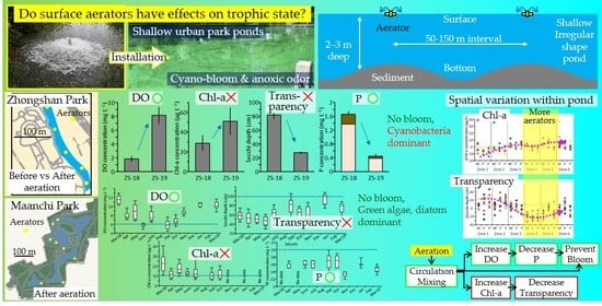
Controlling Eutrophication via Surface Aerators in Irregular-Shaped Urban Ponds

Abstract

Surface aerators have often been introduced in urban ponds for esthetics, but their roles in remediating water quality are less understood. Effects of surface aerators on controlling eutrophication were examined in two urban ponds, in which anaerobic odors and cyanobacterial blooms had occurred and several aerators had been installed. In one of the ponds, a dramatic improvement in dissolved oxygen (DO) (from 1.8 to 8.1 mg L⁻¹) and total phosphorus (TP) (from 1.6 to 0.4 mg L⁻¹) was evident based on the comparison before and after the aeration. Although cyano-bloom did not occur, phytoplankton was dominated by cyanobacteria Microcystis species in both periods. Chlorophyll a (Chl-a) increased (from 29 to 51 μg L⁻¹) and water transparency decreased (from 81 to 27 cm) after the aeration. In the other pond with an irregular shape, water quality was monitored two years after the installation to examine seasonal variation in trophic state and its spatial variation associated with aerator distribution. The water was mixed vertically well for the whole pond, as indicated by small surface-to-bottom differences in temperature. DO decreased in summer after rainfall but was always >5.7 mg L⁻¹. Total nitrogen (TN) and TP were 0.8–2.3 and 0.03–0.07 mg L⁻¹, respectively, and no cyano-blooms were observed across sites throughout the year. Phytoplankton was dominated by green algae and diatom species, which may be favored by the lower phosphorus level of the pond. Chl-a was higher and transparency was lower in the north side, which had more aerators and less shade from trees and buildings. These results suggest that surface aerators increased DO by vertical and horizontal mixing of water, reduced phosphorus release from sediment, and prevented cyano-bloom occurrence, but they did not improve Chl-a level and transparency. Rather, aeration can promote algal growth, and thus, additional purifying measures such as filtration and contact oxidation are required to further improve the trophic state of these ponds.

1. Introduction

Ponds play various roles in urban areas, including contribution to biodiversity as habitat for aquatic species, regulation of stormwater and microclimate, and provision of recreational, cultural, and educational value [1,2,3]. Many urban ponds are under stress due to eutrophication caused by domestic waste inflow or the accumulation of nutrients and organic matter from surrounding lands and the atmosphere [2,4]. The blooms of phytoplankton are representative of severe eutrophication. Ponds lose their esthetic and recreational value due to an unpleasant appearance and odors originating from the blooms. Certain cyanobacteria phytoplankton produce toxins that are potentially hazardous to both ecosystems and human health [5,6,7]. Excess respiration by bloomed phytoplankton and heterotrophic bacteria lead to oxygen depletion, particularly at the bottom, which creates dead zones for fish and other aerobic animals [8,9,10]. A high density of phytoplankton also reduces water transparency, which induces steep vertical light attenuation and inhibits the growth of periphyton and submerged macrophytes at the bottom [11,12].

Various physical, chemical, and biological measures have been employed to remediate the eutrophication of aquatic systems. Constructed wetlands are effective in reducing nutrient input if the external source is concentrated and space is available for installation [13,14,15]. Bottom sediments are an important source of nutrients in lakes and ponds in which nutrients accumulate over a long period [16,17]. The direct removal of sediment by dredging [18] or capping of bottom sediments using geomaterials and chemical agents that induce flocculation and deposition can effectively reduce nutrient loads [19,20,21]. Macrophyte stands have also been introduced to remove nutrients from aquatic systems [14,22]. However, although effective, some of these measures may have detrimental effects on ecosystems by altering the original habitats (e.g., by dredging) or biogeochemical conditions (by using nonnative materials).

Aeration that promotes the spatial mixing of water can improve water quality by enhancing the activities of indigenous organisms and restoring natural purification processes. Aeration or oxygenation, which increases dissolved oxygen (DO) in the bottom layer and reduces nutrient release from sediments, has been widely used and studied in deep reservoirs [23,24,25]. Vertical mixing of water by aeration can also reduce phytoplankton growth, including that of cyanobacteria, and increase water transparency in some cases [25,26]. Aeration is also an essential procedure that has been explored in aquaculture systems and wastewater technologies [27,28]. Aeration systems have also been installed in many ponds in urban parks [29].

Despite the shallowness of water, the stagnant nature of ponds induces thermal stratification, bottom hypoxia, and surface cyanobacterial bloom [29,30,31]. Fountain-type aeration systems that spray water into the air using an impeller [27,29], which primarily disturbs the surface layer, are often installed in park ponds for esthetics. Surging aerators and paddle wheels that directly disturb (splash) surface water by impeller or wheel are often used to increase DO in aquaculture ponds [32,33]. Axial flow pumps that push water downward from surface or direct injection of surface water (or air) into bottom layers have also been adopted in some ponds [27,34]. However, these aeration systems may be insufficient to circulate water for the entire space if ponds have complicated topography characterized by many horizontal and vertical depressions and the distribution of aerators is inadequate to cover the entire pond [34,35,36]. Few studies have examined the effects of aeration on improving the water quality and trophic state of urban ponds.

Our objective was to evaluate the effects of a surficial aeration system on controlling the trophic state of urban ponds. Water quality surveys were conducted in two urban ponds where cyanobacterial bloom had occurred and several aerators were recently introduced. One pond had a straight and long shape and aerators were installed in the middle of the pond. We examined whether the trophic state of pond was improved by aeration based on comparisons of water quality before and after the installation. The other pond had an irregular shape and several aerators were installed near shoreline. We surveyed water quality two years after the installation, and examined whether good conditions were maintained for the whole pond or if water quality varied spatially, associated with the distribution of aerators. As common indicators of lake eutrophication in China and other countries [37,38], DO, chlorophyll a (Chl-a) concentration, water transparency (i.e., Secchi depth) and nutrients (N and P), as well as the occurrence of cyanobacterial blooms, were monitored. Based on these, the abilities and limitations of surficial aeration in improving the water quality of urban ponds were discussed.

2. Materials and Methods

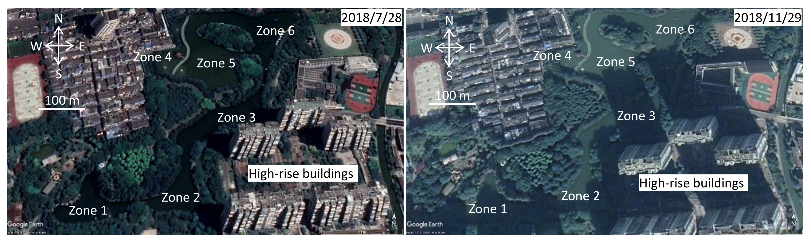
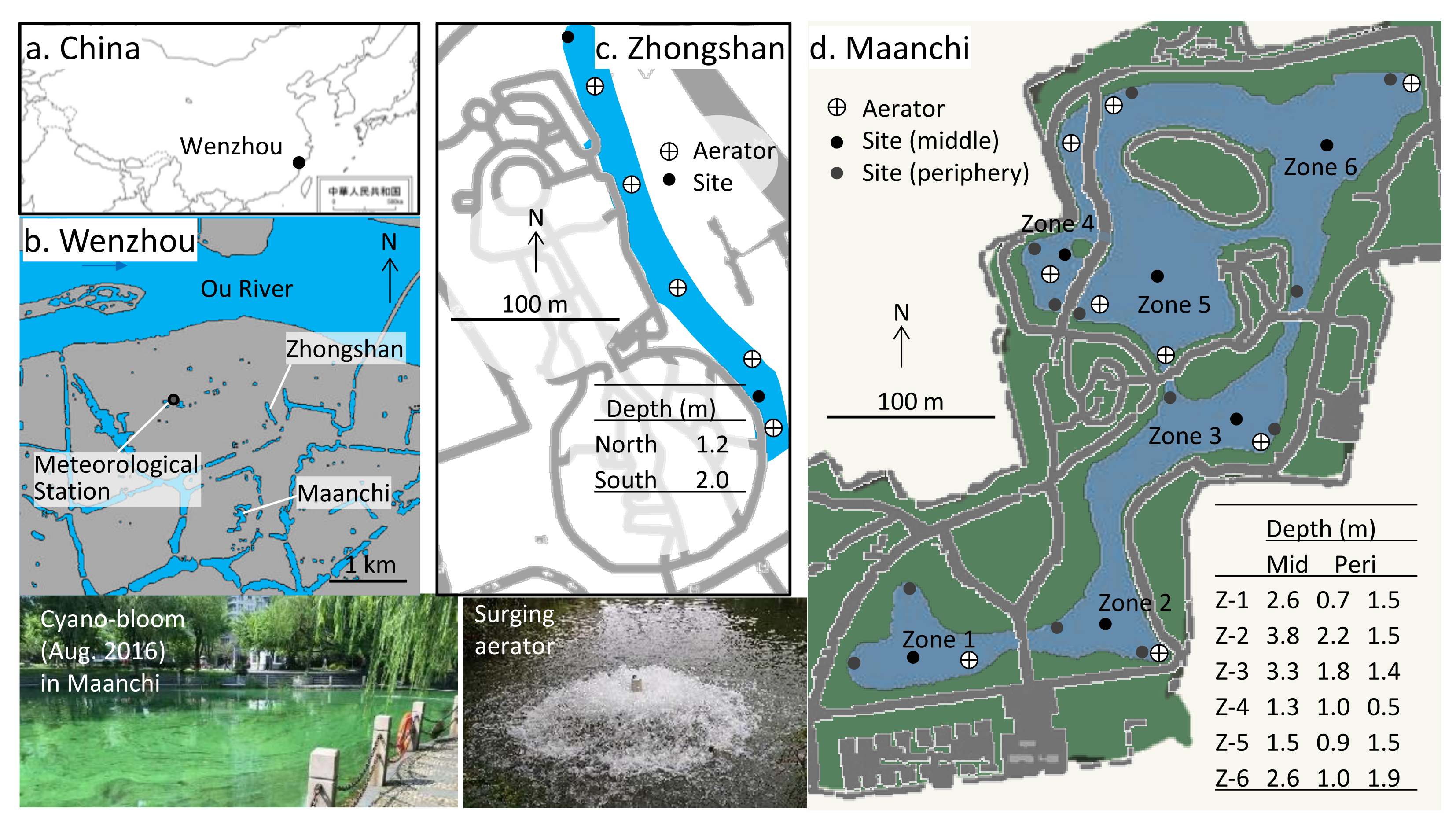
2.1. Site Description

Zhongshan Park (ZS) was located 2.5 km south of the Ou River that flows east near central Wenzhou City, Zhejiang Province, China (Figure 1a,b). The pond was straight and had a simple shape with length and width of 300 m and 20 m, respectively (Figure 1c). It was oriented north–south and located on the east side of the park. Pond depth varied from 1.2 m in the north to 2.0 m in the south. The west side of the park included planted tree stands, open fields, a 40 m high mountain with natural vegetation, and trails connecting different fields. There was no apparent inflow and outflow except two channels, which connected the pond and a nearby river on the west side and were usually dry. Anaerobic odor and cyanobacterial bloom occurred often in ZS. The Wenzhou Park Management Office installed aerators at five locations in the middle of the pond in late 2018. They selected a surge-type aerator (energetic efficiency: 1.5 kg O₂ kw⁻¹ h⁻¹, shaft speed: 500 rpm, YLY-1.5, Zhejiang Fordy Machinery Co., Ltd., Taizhou, China) that upwells water into air by an impeller attached to its shaft and motor (Figure 1). The device was suspended by a floating ring (diameter: 1 m) connected to a triangle-arranged pile. These aerators operated during the daytime, except noon, to reduce noise pollution especially in the nighttime for the residents and throughout seasons.

Maanchi Park (MA) was located 1 km southwest of the ZS. The pond had an irregular shape with a sequence of wide (40–80 m) and narrow (<20 m) zones and occupied the middle of the park (Figure 1d). It was 500 m long and oriented southwest–northeast. Water depth varied from 1.3 m on the northwest side to 3.8 m on the southern side, and it was deeper in the middle than in the periphery. The other areas of the park were tree stands (evergreen, deciduous, and conifer trees), flower gardens, recreational fields, and pondside trails or those connecting different fields. The pond banks were protected from erosion by stones, wooden piles, and concrete walls. The canopy of trees planted along the pond banks overhung and provided shade at the periphery of the pond. There was no apparent inflow or outflow of the pond except when rainfall and surface runoff of the surrounding area partially entered the pond and subsequently drained to nearby small channels through pipes, which were usually above the pond water surface. The park was surrounded by residential buildings. A hundred-meter-class high-rise apartment is concentrated at the southeast side of the park, which shaded the southern half of the pond from direct sunlight in the morning.

Cyanobacteria blooms (Figure 1) had been observed in the pond several times since the 2010s. The pond had often emitted anaerobic odors, and the nutrient level of pond water was high especially for ammonium-N (NH₄⁺-N) and total phosphorus (TP) at least until summer of 2016 (i.e., in the worst category by surface freshwater standard of China, which means NH₄⁺-N and TP were >2.0 mg L⁻¹ and >0.4 mg L⁻¹, respectively). Wenzhou Park Management Office installed the same aerators in 2015 and 2016. Nine aerators were running near shoreline with more in the northwest of the pond (Figure 1d).

2.2. Field Survey

The survey in ZS was conducted in June 2018 and June 2019 (when hypoxic condition and bloom occurrence were mostly expected) corresponding to before and after the installation of aerators, respectively. We visited two sites (Figure 1c) (but access to the north site was prevented by public activities in the second survey). At each site, the vertical profile (0.1 m intervals) of water quality (i.e., electric conductivity = EC, DO, pH, Chl-a, turbidity, and oxidation-reduction potential = ORP) was determined using a multiparameter water quality meter (Hydrolab DS5X including Hach LDO^® sensor; OTT Hydromet GmbH, Kempten, Germany). Water transparency was measured using a Secchi disk. For concentrations of N and P, 100 mL water samples were collected from the surface (at a depth of 0.1 m) and bottom (0.2 m above the bottom) using a resin tube and syringe. The occurrence of cyanobacterial bloom was visually determined for the whole pond, and a water sample for the microscopic analysis of plankton community was collected at the survey sites.

For MA, water quality surveys were conducted two years after the aerator installation, 10 times from March 2018 to March 2019 (i.e., March 2018, April, May, June, July, September, October, November, January 2019, March). The pond was divided into six zones and numbered from southwest to northeast (Figure 1d). Zones 4 and 5 were separated by an embanked trail and connected by culverts under the trail. The two islands in the north bordered zone 5 and zones 3 and 6. A total of 18 monitoring sites were established, one in the middle and two in the periphery of each zone. Water quality measurement and water sampling protocol were the same. Water samples were collected from the six middle sites each month (besides March 2018 and May). All surveys were performed from 12:00 to 17:00 each month. Meteorological data were obtained from the nearest station (Figure 1b).

The concentrations (mg L⁻¹) of total nitrogen (TN) and phosphorus (TP), ammonium-N (NH₄⁺-N), nitrite-N (NO₂⁻-N), nitrate-N (NO₃⁻-N), and soluble reactive phosphorus (SRP) in the collected water samples were determined as described in [39].

2.3. Statistical Analysis

Differences in DO and Chl-a, transparency, TN, and TP before and after the installation of aerators in ZS (ZS-18 and ZS-19, respectively) were examined via one-way ANOVA with unequal sample sizes. Data from two sites for two days in June 2018 (i.e., n = 4) and one site for five days in June 2019 (n = 5) were used. The representative value of each site was obtained by averaging 0.1 m interval data or surface and bottom data.

In MA, the mean value for each field-measured variables (i.e., temperature, EC, DO, pH, Chl-a, turbidity, and ORP) was obtained for each site from vertical 0.1 m interval data. The mean value was used to examine the spatial (horizontal) variation of water quality using linear mixed-effects models with survey month (10 months), zone (6 zones), and lateral position (middle, periphery) as fixed factors and site (18 sites) as the random factor. Chl-a data were only available for seven months because of sensor equipment issues in the last three months. The surface-to-bottom layer difference (Δ_layer) was also calculated for each variable using the mean of surface (0–0.5 m) and bottom (0.5 m near bottom) of each site to comprehend the magnitude of vertical difference. Because the vertical change was not always a monotonic decrease or increase in Chl-a, the depth of maximum Chl-a (Chl-a maximum, D_Chl-max) was also determined for each site. Spatial variations in nutrient concentrations (TN, NH₄⁺-N, NO₂⁻-N, NO₃⁻-N, TP, and SRP) were examined using a three-way analysis of variance (ANOVA) without replication (n = 1) using month (8 months), zone (6 zones), and layer (surface and bottom) as factors.

Principal component analysis (PCA) using a correlation matrix was performed to investigate the relationships among the field-measured variables in space and time in MA. For spatial patterns, PCA was performed among 18 sites for each month. The mean value of vertical 0.1-m interval data was used for each variable at each site. For temporal patterns, water quality data were averaged among 18 sites to obtain a representative value for each month, and PCA was performed among all months. Due to a lack of data for three months, Chl-a was omitted from this analysis. The scores of the first and second axes obtained by PCA were used as the water quality state of each month, and correlations between these scores and meteorological variables were examined using the Pearson product-moment correlation coefficient (r). Data on daily rainfall, sunlight hours, air temperature, and wind speed were summed or averaged for seven days preceding the survey to obtain representative values for each month.

For all tests, an α value of 0.05 was used to determine the significance of the effects. All statistical analyses were performed using R software (version 4.0.3; R Development Core Team, Vienna, Austria) with the packages of “lme4” and “lmerTest.”

3. Results

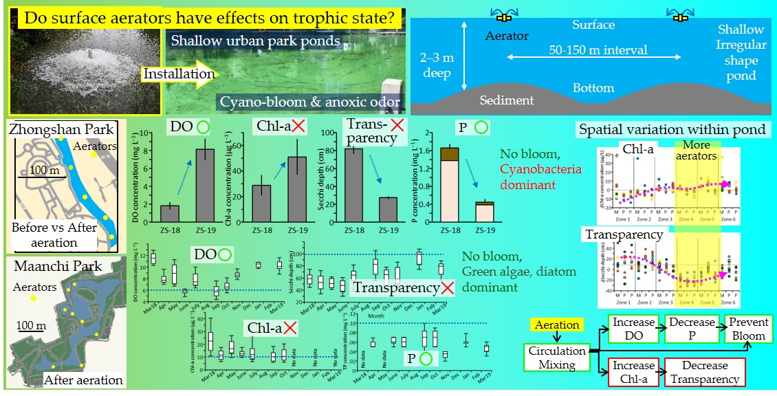
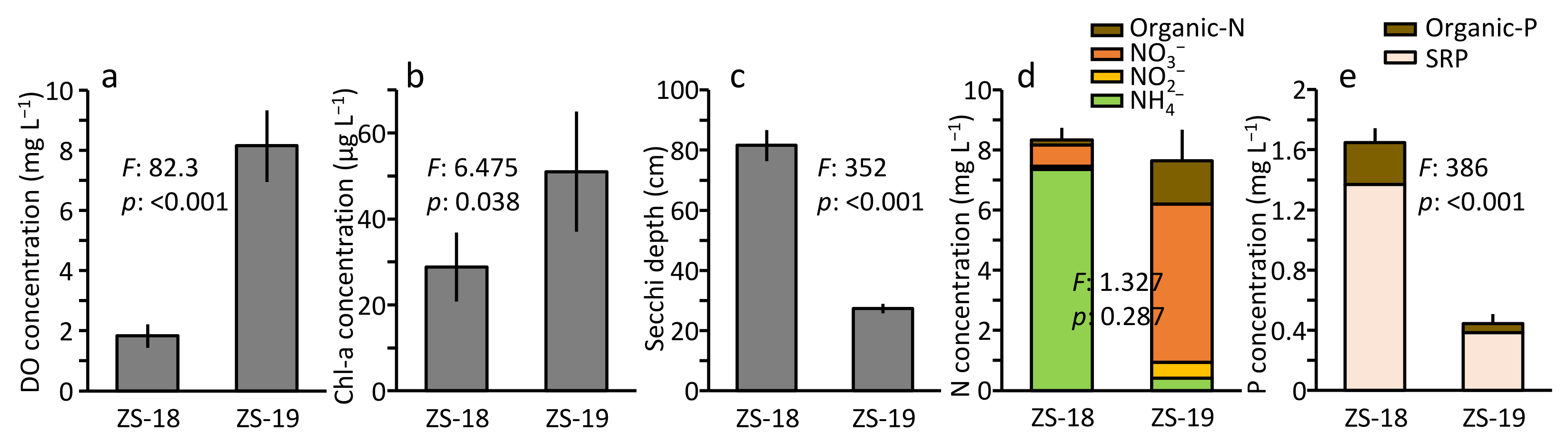
3.1. Changes in Water Quality in ZS Pond

Changes in water quality by installation of aerators were suggested by significant differences between ZS-18 (before installation) and ZS-19 (after installation) (Figure 2). The concentration of DO in ZS-19 (8.1 ± 1.2 SD mg L⁻¹) was significantly higher than and more than 4-fold of that in ZS-18 (1.8 ± 0.4 mg L⁻¹) (Figure 2a). The Chl-a in ZS-19 was significantly higher than that in ZS-18 (Figure 2b). By contrast, transparency in ZS-19 was significantly lower than that in ZS-18 (Figure 2c). The concentration of TN differed less between ZS-18 and ZS-19 (Figure 2d). Despite the small difference in TN, its composition was changed; the concentrations of NH₄⁺ decreased by simultaneous elevation of NO₃⁻. The concentration of TP in ZS-19 (0.44 ± 0.07 mg L⁻¹) was significantly lower than and one-fourth of that in ZS-18 (1.64 ± 0.09 mg L⁻¹) (Figure 2e).

Anaerobic odors were detected only in ZS-18. No cyanobacterial bloom was observed for the whole pond in both periods. However, cyanobacteria Microcystis species (M. aeruginosa in ZS-18, M. aeruginosa and M. wesenbergii in ZS-19) was abundant and dominated phytoplankton in both periods (Table S1).

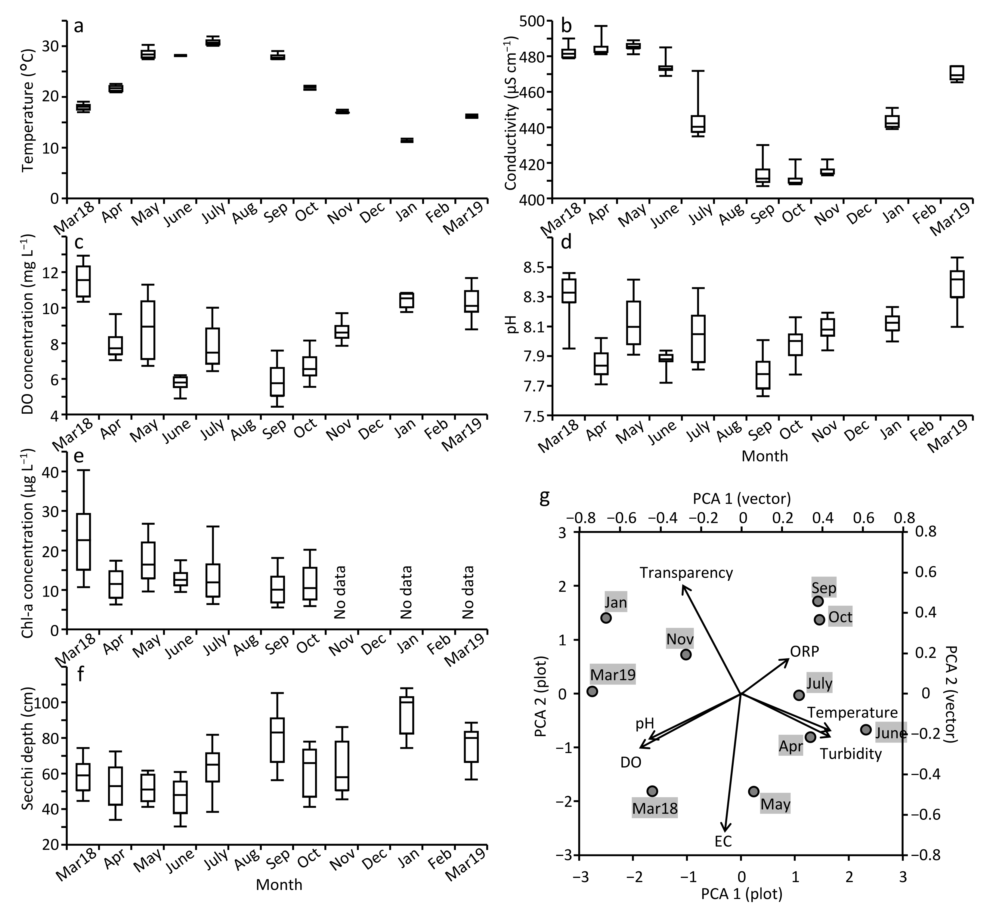
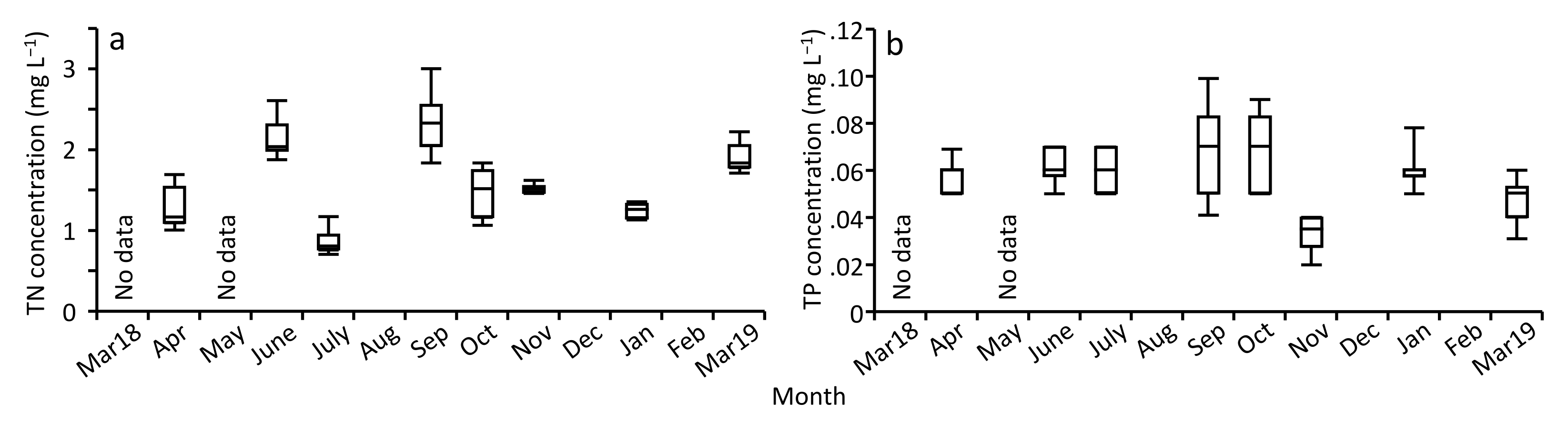
3.2. Temporal Changes of Water Quality in MA Pond

The mean air temperature of Wenzhou City changed from 14.3 °C (±5.2 SD) in March 2018 to 28.6 °C (±1.3) in August and then decreased to 10.9 °C (±2.2) in January (Figure S1). Rainfall increased from late April to September. Daily sunlight hours were lower in winter, from December to February. The predominant wind was easterly except in winter with predominantly north wind.

Water temperature (Figure 3a) showed a seasonal pattern similar to air temperature (Figure S1) and was 0.8–4.9 °C higher for water than air each month. A short box each month indicates that the spatial variation of temperature was less than the seasonal variation (Figure 3a). EC decreased steeply from 474 μS cm⁻¹ in June to 416 μS cm⁻¹ in September and increased after November (Figure 3b). The DO concentration decreased from 11.5 mg L⁻¹ in March 2018 to 5.8 mg L⁻¹ in June and September, and then increased to 10.1–10.5 mg L⁻¹ in January and March 2019 (Figure 3c). A long box indicates that the spatial variation of DO was large. The seasonal change in pH (7.7–8.4) (Figure 3d) was similar to that of DO. Chl-a concentration was >10.4 μg L⁻¹ in all measured months, and it was 16.4–22.6 μg L⁻¹ in March 2018 and May (Figure 3e), when DO and pH were also high. Turbidity ranged 17.0–20.3 nephelometric turbidity units (NTU) from March 2018 to October with no clear seasonal trend. Water transparency increased from 48–59 cm in the first four months to 80–100 cm in September, January, and March 2019 (Figure 3f). A long box each month in pH, Chl-a, and transparency indicates a large spatial variation relative to temporal variation.

In the PCA of water quality variables among the 10 surveyed months, the first and second axes accounted for 71.5% of the total variance (Figure 3g). The first axis was positively correlated with water temperature and turbidity and negatively correlated with DO and pH. The second axis was positively correlated with transparency and negatively correlated with EC. Months were plotted counterclockwise, with the first month (i.e., March 2018) in the third quadrant, and late spring to early autumn months had positive PCA1 scores. Among the four meteorological variables, the first axis of the PCA was correlated most strongly with air temperature (Pearson’s r = 0.75, p = 0.012), followed by rainfall (r = 0.64, p = 0.046), and the second axis correlated most strongly with sunlight hours (r = −0.56, p = 0.091). Overall, this implies that DO and pH tended to be low from late spring to early autumn months when air temperature and rainfall were high, and transparency tended to be low in spring and early summer months when EC was high.

Nutrient concentrations varied among months, but no clear seasonal trend was observed (Figure 4 and Figure S2). For example, TN varied from 0.80 to 2.33 mg L⁻¹ and was higher in June and September than in the other months (Figure 4a). NH₄⁺-N was higher in April, September, and October (0.21–0.26 mg L⁻¹) compared to the other months (0.10–0.16 mg L⁻¹), whereas NO₃⁻-N was higher in April, November, and March 2019 (0.64–1.01 mg L⁻¹) than the other months (0.34–0.48 mg L⁻¹). TP varied from 0.035 mg L⁻¹ in November to 0.070 mg L⁻¹ in September and October (Figure 4b). SRP was higher in July, September, October, and January (0.045–0.060 mg L⁻¹) than in the other months (0.025–0.040 mg L⁻¹).

Cyanobacterial bloom was not observed at any sites during the study in MA. The phytoplankton community collected for a single time in May was dominated by green algae and diatom species. Cyanobacteria Microcystis species, which were abundant in the ZS pond, were not found (Table S1).

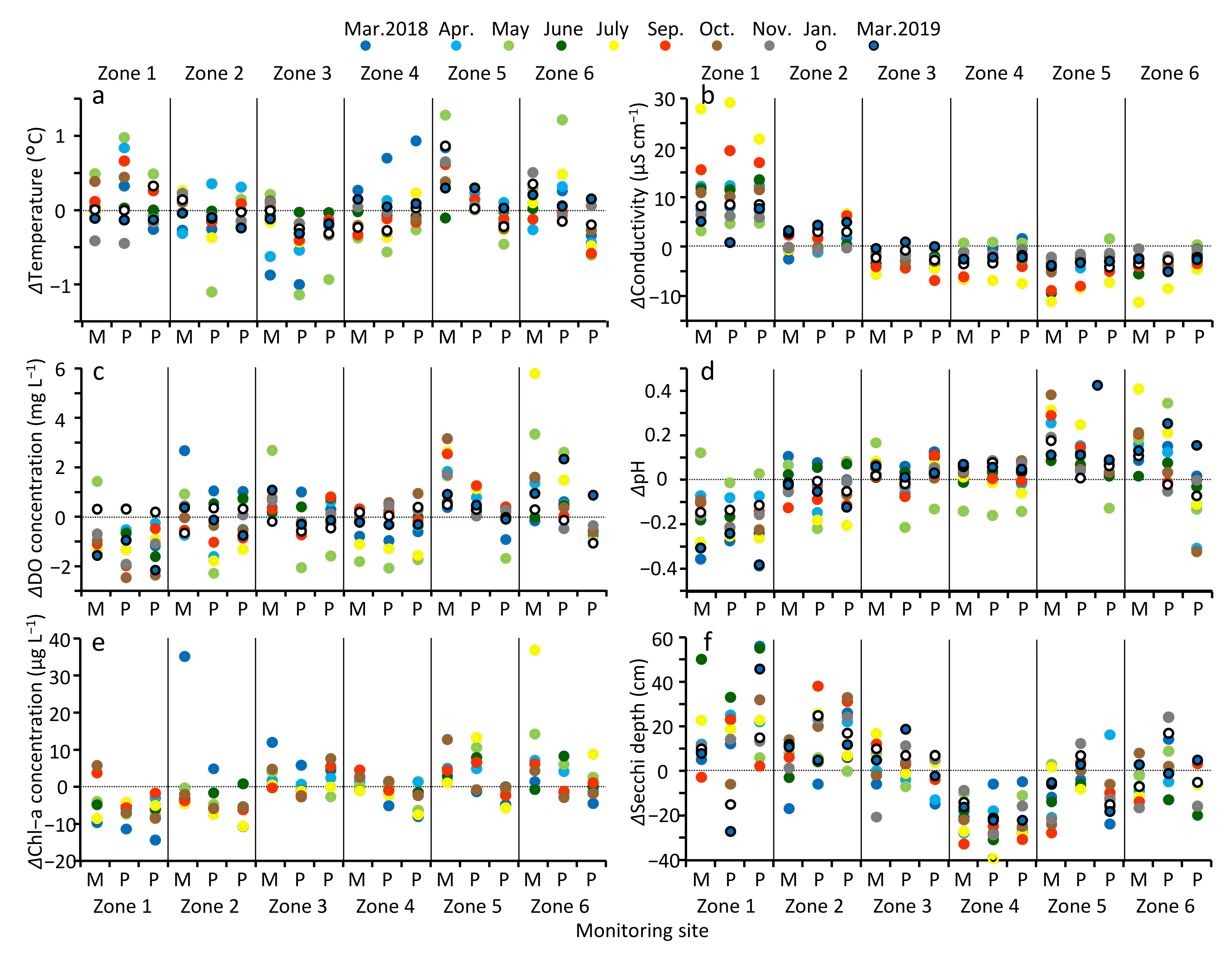
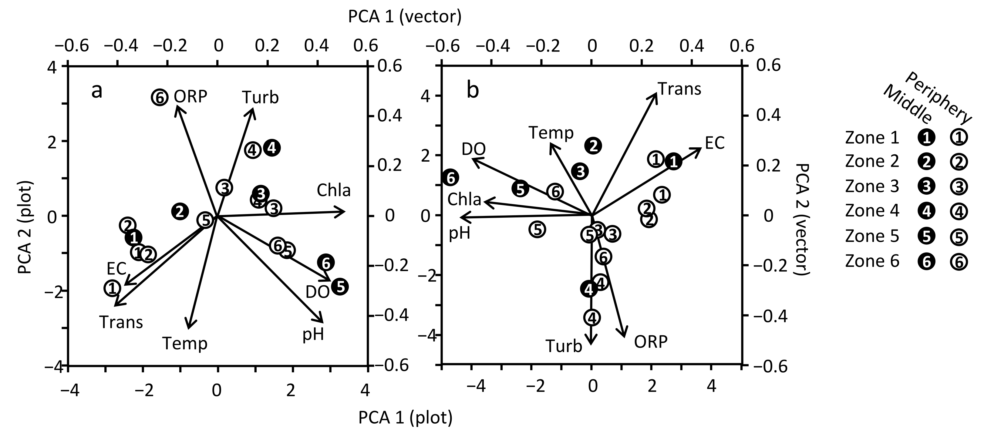
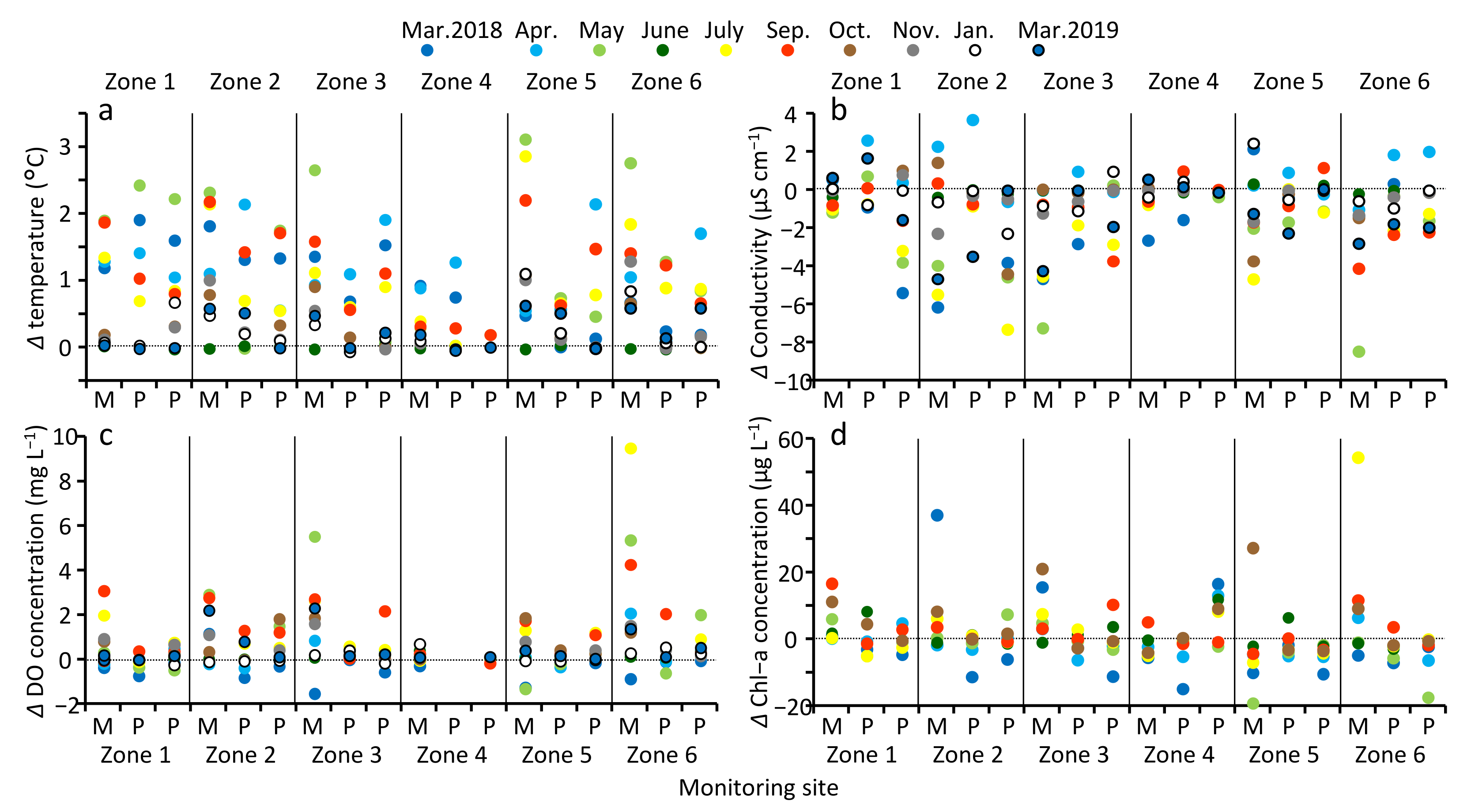
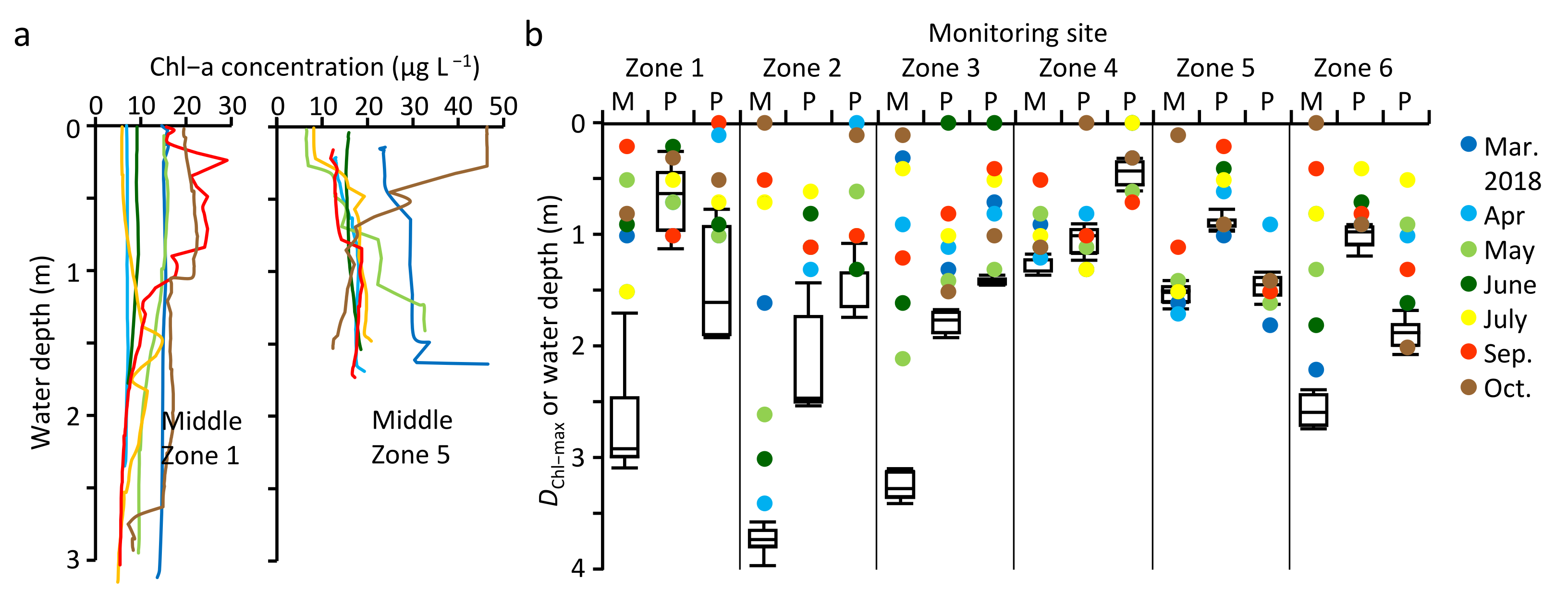
3.3. Spatial Variation of Water Quality in MA

Most water quality variables significantly varied among the six zones and between the lateral positions in each zone across the survey months (

Table 1. Mean values of water quality variables at each zone and lateral position in MA, and results of linear mixed-effects model. T: temperature, SD: transparency.

	Mean across All Months										LME Model Results (F 2, p 3)
	Zone							Position			Factors 1
	1	2	3	4	5	6		Mid.	Peri.		M	Z	P	M × Z	M × P	Z × P
T (°C)	22.4	22.2	22.0	22.2	22.5	22.3		22.4	22.2		>99	2.58	2.52	1.80	2.81	1.45
EC (μS cm−1)	463	454	450	450	448	449		452	453		>99	>99	5.37	17	1.42	0.49
DO (mg L−1)	7.49	8.28	8.51	8.07	9.04	9.00		8.90	8.15		>99	6.08	11	6.35	7.17	1.23
pH	7.89	8.02	8.09	8.08	8.18	8.13		8.11	8.04		>99	8.01	4.61	2.96	2.34	0.67
Chl-a (μg L−1)	9.6	12.6	17.2	14.0	17.9	19.1		18.2	13.5		35	4.83	11	5.80	5.57	0.69
Turbidity (NTU)	18.9	16.4	16.0	23.1	16.6	17.8		18.2	18.1		53	10	0.01	12	5.41	2.61
ORP (mV)	426	425	440	456	442	442		416	450		17	3.66	33	2.06	3.32	2.63
SD (cm)	85	82	70	46	61	67		66	70		20	10	1.48	1.31	1.76	0.41

¹ Fixed factors in linear mixed-effects model, M: month, Z: zone, P: lateral position. ² F-values with 3 or 4 digits are shown as >99. ³ Bold: p < 0.001, double underlines: p < 0.01, single underline: p < 0.05.

). To clearly focus on spatial variation, the difference from the mean of each month is shown in Figure 5. Water temperature varied less among zones and between the positions (Table 1, Figure 5a). EC was the highest in zone 1, followed by zone 2, throughout the year (Figure 5b). The difference among zones was especially large in some months (such as July and September, Figure 5b), which was indicated by the significant month × zone interaction (Table 1). DO concentration was highest in zones 5 and 6, and lowest in zone 1 (Figure 5c). Such differences were large in some months (such as July and October), which was indicated by the significant month × zone interaction. DO was also significantly higher in the middle than in the periphery. The spatial pattern of pH was similar to that of DO, highest in zones 5 and 6, and lowest in zone 1 (Figure 5d). The Chl-a concentration was highest in zone 6, followed by zone 5, and lowest in zone 1, followed by zone 2 (Figure 5e), with almost two-fold difference between zones 1 and 6 (Table 1). However, such differences were small in some months (such as June and September), which was indicated by the significant month × zone interaction. Chl-a was also higher in the middle than periphery. Turbidity was highest in zone 4, followed by zones 1 and 6 (Table 1). The ORP was highest in zone 4 and lowest in zone 2 in some months. Water transparency was highest in zone 1, followed by zone 2, and lowest in zone 4, followed by zone 5 (Figure 5f), with nearly two-fold difference between zones 1 and 4 (Table 1).

In the PCA of water quality variables, the first and second axes accounted for 67.1–80.2% (mean: 72.1%) of the total variance among 18 sites for each month (Figure 6 and Figure S3). In many months, the first axis was positively or negatively correlated with DO, pH, Chl-a, EC, and transparency in opposite directions between the former three and the latter two. The second axis was positively or negatively correlated with temperature and ORP in many months, and sometimes with turbidity. Plots of the 18 sites were usually distributed with the middle and periphery sites of zone 1 and 2 at one end, and the middle site of zone 5 or 6 at the other end along the first axis (Figure 6a,b). The middle site of zone 4 was always on the other side of zone 1 and 2 along the first or second axis, and it also tended to separate from the middle site of zone 5 and 6 along the second axis. The middle and periphery sites tended to be separated along the second axis, except for the middle site of zone 4 (Figure 6b and Figure S3). In summary, zones 1 and 2 had lower DO, pH, and Chl-a and higher EC and transparency than zones 4, 5, and 6, and the middle site of zone 4 and the periphery site of all zones had higher ORP and turbidity than the other middle sites.

The vertical difference (i.e., Δ_layer) of water temperature was less than 2 °C at most sites (Figure 7a), and it was always less than 1 °C in zone 4, where the water depth was small. The positive Δ_layer suggests that the temperature was always higher at the surface than at the bottom. The Δ_layer of EC was usually −4–1 μS cm⁻¹ (Figure 7b), which was small compared to the horizontal variation (Figure 5b). The Δ_layer of DO was usually −0.5–2 mg L⁻¹ (Figure 7c), which was small compared to the horizontal variation, whereas it occasionally exceeded 4 mg L⁻¹ at the middle site of zone 6. Similarly, the Δ_layer of pH was usually 0–0.3, whereas it occasionally exceeded 0.4 at the middle site of zone 6. The Δ_layer of Chl-a was usually −5–10 μg L⁻¹ (Figure 7d). The vertical differences in turbidity and ORP were usually −2–0 NTU and −5–1 mV, respectively. Overall, vertical differences in water quality variables were usually small.

As mentioned, the vertical change was not always a monotonic decrease or increase in Chl-a (Figure 8a). At each site, Chl-a maximum (D_Chl-max) usually varied within the upper half layer (e.g., the middle sites of zones 1 and 3) or widely from the surface to bottom (e.g., the middle sites of zones 2 and 6, Figure 8b), whereas it was concentrated near the bottom in the middle sites of zones 4 and 5 and some periphery sites that were located nearby the aerators in zones 4, 5, and 6 (Figure 8b).

Concentrations of TN and TP varied significantly among months, whereas they varied less among zones and between layers (

Table 2. Mean values of N and P concentrations (mg L⁻¹) at each zone and each layer in MA, and results of a three-way ANOVA without replication.

	Mean across All Months										ANOVA Results (F 2, p 3)
	Zone							Layer			Factors 1
	1	2	3	4	5	6		Surf.	Bott.		M	Z	L	M × Z	M × L	Z × L
TN	1.769	1.749	1.637	1.544	1.524	1.611		1.657	1.621		28	1.34	0.25	1.58	2.11	2.18
NH4+-N	0.173	0.231	0.165	0.152	0.179	0.152		0.163	0.188		11	5.08	5.55	4.23	0.36	1.31
NO2−-N	0.025	0.030	0.028	0.027	0.028	0.028		0.027	0.028		>99	11	3.03	5.34	1.80	1.69
NO3−-N	0.619	0.576	0.549	0.516	0.548	0.543		0.550	0.567		>99	4.63	1.61	2.58	1.95	1.30
TP	0.068	0.061	0.057	0.053	0.050	0.063		0.059	0.058		3.50	2.36	0.08	1.05	2.20	0.68
SRP	0.055	0.043	0.037	0.034	0.038	0.048		0.043	0.041		5.58	4.05	0.43	0.96	1.77	0.76

¹ Fixed factors in ANOVA, M: month, Z: zone, L: layer. ² F-values with 3 or 4 digits are shown as >99. ³ Bold: p < 0.001, double underlines: p < 0.01, single underline: p < 0.05.

). The concentration of NH₄⁺-N varied significantly among zones, being highest in zone 2 and lowest in zones 4 and 6. The difference was more obvious in some months (such as November, January, and March 2019), as indicated by the significant month × zone interaction. It was also significantly higher for bottom than surface. The concentration of NO₃⁻-N varied significantly among zones, being highest in zone 1 and lowest in zone 6. The difference was more obvious in some months (such as April, January, and March 2019). The concentration of SRP varied significantly among zones, being highest in zone 1 and lowest in zone 4. In summary, all nutrient variables except NO₂⁻-N were slightly (11–25%) higher in zones 1 and 2 than in zones 4, 5, and 6 especially in winter and early spring months.

4. Discussion

In this study, water quality was monitored in two urban ponds, where cyanobacterial bloom had occurred and multiple surficial aerators were introduced afterward. A dramatic increase in DO and reduction in concentrations of TP after the aerator installation in ZS suggests that the aerators can greatly improve eutrophic states associated with hypoxic conditions. In MA, two years after the installation, hypoxic conditions, cyanobacterial blooms, and high nutrient levels, which were previously reported, were not evident at any sites through year, which suggests that the aerators were effective at preventing those occurrences even though the pond has an irregular shape. It should be noted that the improved status lasts as long as the aeration is operated. In addition, Chl-a was high and water transparency was low in ZS and zones with more aerators in MA, which suggests a limitation of aerators for improving some eutrophic indicators.

4.1. Changes in Water Quality by Aerators in ZS

The water quality of ZS was shown to have changed dramatically by the installation of the aerators. The concentration of DO suggests that the pond water changed from hypoxic to aerobic for the entire depth after installation. Observationally, no anaerobic odor was detected during the surveys in 2019. In addition, substantial reductions in the concentrations of SRP after the installation suggests that phosphorus released from the mud to the overlying water was reduced by the change in oxygen conditions [40,41]. We considered that previously released phosphorus had been assimilated by phytoplankton and heterotrophic microorganisms and deposited. Although NH₄⁺-N, which can be released from mud under hypoxic conditions [42,43], also decreased substantially after the installation, TN did not decrease due to NO₃⁻-N increase.

Despite the phytoplankton community being dominated by cyanobacteria Microcystis species both before and after the installation, we did not observe cyanobacterial surface blooms in both periods. However, there is a potential for a surface bloom formation implied by an observation of the bloom in mesocosms installed in ZS in our other study (i.e., using same water but free of circulation by aerators [44]). It is suspected that the high nutrient levels, especially phosphorus, even after the installation (TP: 0.44 ± 0.07 mg L⁻¹, TN/TP ratio: 17.4 ± 3.2) favored the dominance of Microcystis in ZS [45,46]. Instead, water circulation by surface aerators might have disturbed and prevented the bloom formation.

4.2. Water Quality through Year in MA

Anaerobic odors and high levels of ammonium and TP, which had been reported previously, were not detected during our surveys in MA. The concentration of DO was greater than 10 mg L⁻¹ in winter and early spring. It decreased to less than 6 mg L⁻¹ during summer, especially in months when preceding rainfall was high, but it never fell below 2–3 mg L⁻¹, which led to hypoxic water at the bottom.

Concentrations of TN and TP in MA ranged from 0.8–2.3 mg L⁻¹ and 0.03–0.07 mg L⁻¹, respectively, and were near or below the threshold for cyanobacterial bloom occurrence (TN: 1.8 mg L⁻¹, TP: 0.1 mg L⁻¹, [47]). Seasonality was less clear for TN and TP and for each inorganic form. On the other hand, EC showed a clear seasonality and was high in spring and low in autumn. These results contrast with those of other studies that showed higher EC and higher concentrations of N and P in the rainy season due to high nutrient loads from the watershed [48,49]. Thus, seasonal nutrient loads, which could stimulate a temporal bloom occurrence, were not evident in MA. Minerals (e.g., Ca, Mg) that can elevate EC may be supplied by groundwater more in dry season (i.e., winter) and were gradually diluted in rainy season (summer).

Cyanobacterial bloom was not observed at any sites throughout year in MA. The cyanobacteria group Microcystis, which is often dominant in the region, adapts to moderate to high temperatures and grows actively when the water temperature exceeds 20 °C [45,50]. In MA, the water temperature exceeded 20 °C from April to October, which seems to be the potential months for the bloom occurrence. However, Microcystis did not occur and the phytoplankton community was dominated by green algae and diatom species in May, which contrasts with the dominance of Microcystis in the same season in ZS. The lower phosphorus level in MA (TP: 0.06 ± 0.01 mg L⁻¹, TN/TP ratio: 27.7 ± 9.6) might have contributed to preventing the dominance of cyanobacteria.

Results of the two ponds suggest that nutrient level, especially phosphorus, and cyanobacterial bloom occurrence were improved by multiple surface aerators that generated aerobic conditions for the whole pond, even when the ponds had an irregular shape. The difference in the dominance of cyanobacteria in the phytoplankton community between the two ponds may be associated with background nutrient level. Furthermore, the difference in nutrient level between the two ponds may be associated with the time since the aerator installation; the survey was conducted less than one year after installation in ZS and two years after the installation in MA. In ZS, TN (3.8–4.4 mg L⁻¹) and TP (0.33–0.40 mg L⁻¹), which were lower than our survey, were recorded in the next month. In MA, TN (0.30–1.91 mg L⁻¹) and TP (0.05–0.07 mg L⁻¹), which were similar to or slightly lower than our survey, were recorded in the next year. Thus, our survey was possibly conducted in a nutrient-decreasing phase after the installation and was unable to show the full impact of aerators, especially in ZS.

On the other hand, aerators had no effect of improving the concentration of Chl-a and water transparency. Rather, they may deteriorate these conditions. In ZS, these conditions got worse after the installation of aerators. In MA, these conditions were worse in zones with more aerators. In a fish farm pond, a moving surface aerator succeeded to eliminate cyanobacterial bloom, while it slightly increased phytoplankton biomass [36], which is similar to our results. Effects of aerators on Chl-a and the transparency will be further discussed in the following section.

4.3. Spatial Variation of Water Quality in MA

A strong vertical structure was not observed for most water quality variables in MA through the year. Thermal stratification and vertical differences in concentrations of DO and nutrients, especially in summer months, have been reported in shallow ponds with and without an aeration system [30,35,51]. In these studies, surface-to-bottom temperature differences often exceeded 3–4 °C, with reduced DO and elevated nutrient levels at the bottom. By contrast, the surface-to-bottom difference in MA was small for water quality variables including temperature (<2 °C), DO (<2 mg L⁻¹) (Figure 7), and nutrient concentrations (Table 2). Therefore, the installed aerators succeeded in mixing water vertically for the whole pond area, even though each aerator splashed water only at the surface and the topography of pond was complicated with many horizontal and vertical depressions.

Despite the water circulation for the whole pond, high Chl-a concentrations and low water transparencies were evident, particularly in the north side of MA. Groundwater seepage with high mineral concentrations that elevated EC in zones 1 and 2 in the south might have also increased transparency without stimulating algal growth and increasing Chl-a. Chl-a concentration was highest in zones 5 and 6, and transparency was lowest in zone 4 in the north. Because differences in nutrient concentrations between north and south were small (Table 2), the higher Chl-a and lower transparency in the north were less associated with nutrient availability.

The availability of solar radiation for algal photosynthesis may be high in the north side of MA because of few shades on the water. The Chl-a concentration was shown to be lower at the periphery, which was often partly shaded by trees on the bank, than in the middle (Table 1, Figure 5e). Previous studies have shown that, in small streams and ponds in forests, the removal of canopies along the shore often increases solar radiation and primary production of periphyton and phytoplankton [52,53]. In MA, the water area was wide and can receive sunshine for a long time on the north side, especially in zones 5 and 6. In addition, in the north side there were few adjacent high-rise buildings, which block direct sunshine in morning time (Figure 9).

The higher Chl-a and lower transparency in the north side of MA was partially associated with the distribution of aerators. Zones 4 and 5 had more aerators for their water volume than the other zones, and thus the rate of water circulation was greater. Transparency was lowest and the turbidity was highest in zone 4, which had two aerators within a small and shallow area (Figure 1d). In such place, circulation may cause the resuspension of organic matter from the bottom [25,26]. Greater circulation in zones 4 and 5 can also increase algal growth and Chl-a concentrations, which can then decrease transparency. In raceway ponds of algal cultivation, vertical mixing is an essential method to regularly lift algal cells to the surface layer with sufficient light and supply CO₂, which controls algal production and maintains a suitable pH level in the water [28,54]. In a fish farm pond, phytoplankton biomass and algal diversity increased two years after the installation of a moving aerator [36]. In MA, it is notable that vertical Chl-a maxima was near the bottom in zones 4 and 5, which contrasted with the surface or dispersed vertical maxima in the other zones (Figure 8b). Algae with less floating abilities may be supported by the circulation in zones 4 and 5. Further examination is needed to understand whether algal growth can be prevented or promoted by water circulation in urban ponds.

The higher DO in the north side may be associated with photosynthesis by phytoplankton. The aeration elevated the basic DO level to more than 5–6 mg L⁻¹ even in summer months for the whole pond in MA. Meanwhile, DO varied spatially, being higher in the north than in the south zones (Figure 3 and Figure 5), and it always correlated positively with Chl-a and pH (Figure 6), which supports DO increase by algal photosynthesis. Notably, despite the location of aerators at periphery, DO, Chl-a, and pH were higher in the middle than the periphery. These findings suggest that the spatial variations in DO were more affected by the difference in photosynthesis rather than difference in DO diffusion by aeration.

Although there was no apparent inflow and outflow in MA, there may be a certain horizontal circulation. During the surveys, local movements of surface water induced by winds or aerator-generated waves were visible based on floating leaves as tracers. In shallow lakes, a wind-induced horizontal circulation often occurs with a main flow along the shoreline in the wind direction and a return flow in the center [55,56,57]. The wind direction was predominantly east (i.e., heading west) in most months in Wenzhou (Figure S1), and the effects of wind were likely to be stronger in the north than in the south because of the wider water area with less wind-breaking trees and high-rise buildings (Figure 9). Accordingly, there may be a wind-induced westward flow toward zone 5 from zone 6, and a return flow that goes back to zone 6 from zone 5 through the islands or via zone 3. Water in zones 1–3 may be prone to being stagnant without aerators.

4.4. Limitations and Possibilities of Surface Aerators

Surface aerators are ubiquitous in park ponds for esthetics in many cities. Irrespective of the purpose of installation, surface aerators have certain roles of circulating water and increasing DO that can improve eutrophic states associated with hypoxic conditions in urban ponds. However, the effectiveness of circulation varies according to the type of aerator. Although fountain type aerators are popular in parks, a limited vertical mixing and effect on cyanobacteria has been reported in a pond and shallow lake [29,35]. Axial flow pumps that push water downward from surface produce excessive turbulence and local circulation in a shallow and flat bottom, which resulted in very low efficiency in circulating water for an entire lake [34]. Paddle wheels and surging aerators, which are often used in aquaculture ponds [32,33], may have similar circulation efficiencies. A centrifugal water stirrer, which was intended to push water radially on surface, circulated water horizontally and vertically much more efficiently than paddle wheels in an aquaculture pond [33]. These studies may suggest that aerators that push water horizontally rather than vertically work well for the circulation of whole water bodies in ponds.

Our study also indicates that even under sufficient circulation, aerators have less effects on improving Chl-a concentration and transparency. Rather, aerators may contribute to increasing Chl-a and decreasing transparency through stimulating algal growth and promoting resuspension of organic matter from the bottom. Because we did not measure suspended solids, we could not distinguish whether the decreased transparency was due to turbid (inorganic) substances or algal-derived organic matter. In reservoirs and lakes, both increased and decreased cases of Chl-a concentration and water transparency after aeration have been reported [25,26].

Filtration and contact oxidation are processes that can remove organic matter from water via circulation. Our other study in ZS [44] suggested that a circulation device equipped with contact oxidation carriers, which filtrate and degrade organic matter, can effectively reduce Chl-a concentration and increase transparency in pond mesocosms. An increase in transparency is key to the growth of periphyton and submerged macrophytes [11,12,39], which further improves water quality and offers habitats and food for fish and other aerobic animals. Thus, to further improve the trophic state and enhance the aquatic community in urban ponds, we recommend adding devices that filter circulated water and remove organic materials on existing aeration systems rather than increasing the number or power of aerators.

5. Conclusions

Surface aerators have been introduced in many urban ponds for esthetics, but their roles on modifying water quality are less known. Water quality was monitored in two urban ponds, where surface aerators were introduced to prevent cyanobacterial blooms. Results from the two ponds suggest that the aerators succeeded in mixing pond water vertically and horizontally well even though the pond had an irregular shape, improved or maintained DO concentrations in moderate to high levels and nutrient concentrations in moderate to low levels, and prevented the occurrence of cyanobacterial bloom. However, the two ponds differed in the dominance of cyanobacteria in the phytoplankton community, which may be associated with the nutrient level and the time since the aerator installation. In addition, aerators can deteriorate trophic state by increasing Chl-a concentration and decreasing transparency. Because algal growth can be promoted by water circulation, additional purifying processes such as filtration and contact oxidation are required to further improve the trophic state of these ponds.

References

1. Hassall, C. The ecology and biodiversity of urban ponds. Wiley Interdiscip. Rev. Water 2014, 1, 187–206. [Google Scholar] [CrossRef]
2. Waajen, G.W.A.M.; Faassen, E.J.; Lürling, M. Eutrophic urban ponds suffer from cyanobacterial blooms: Dutch examples. Environ. Sci. Pollut. Res. 2014, 21, 9983–9994. [Google Scholar] [CrossRef] [PubMed]
3. Oertli, B.; Parris, K.M. Toward management of urban ponds for freshwater biodiversity. Ecosphere 2019, 10, e02810. [Google Scholar] [CrossRef] [Green Version]
4. Smith, V.H.; Schindler, D.W. Eutrophication science: Where do we go from here? Trends Ecol. Evol. 2009, 24, 201–207. [Google Scholar] [CrossRef]
5. Ibelings, B.W.; Chorus, I. Accumulation of cyanobacterial toxins in freshwater “seafood” and its consequences for public health: A review. Environ. Pollut. 2007, 150, 177–192. [Google Scholar] [CrossRef]
6. Cheung, M.Y.; Liang, S.; Lee, J. Toxin-producing cyanobacteria in freshwater: A review of the problems, impact on drinking water safety, and efforts for protecting public health. J. Microbiol. 2013, 51, 1–10. [Google Scholar] [CrossRef] [PubMed]
7. Rousso, B.Z.; Bertone, E.; Stewart, R.; Hamilton, D.P. A systematic literature review of forecasting and predictive models for cyanobacteria blooms in freshwater lakes. Wat. Res. 2020, 182, 115959. [Google Scholar] [CrossRef] [PubMed]
8. Helminen, H.; Karjalainen, J.; Kurkilahti, M.; Rask, M.; Sarvala, J. Eutrophication and fish biodiversity in Finnish lakes. SIL Proc. 1922–2010 2000, 27, 194–199. [Google Scholar] [CrossRef]
9. Gong, Z.; Xie, P. Impact of eutrophication on biodiversity of the macrozoobenthos community in a Chinese shallow lake. J. Freshw. Ecol. 2001, 16, 171–178. [Google Scholar] [CrossRef] [Green Version]
10. Glibert, P.M. Eutrophication, harmful algae and biodiversity—Challenging paradigms in a world of complex nutrient changes. Mar. Pollut. Bull. 2017, 124, 591–606. [Google Scholar] [CrossRef]
11. Vadeboncoeur, Y.; Jeppesen, E.; Zanden, M.J.V.; Schierup, H.H.; Christoffersen, K.; Lodge, D.M. From Greenland to green lakes: Cultural eutrophication and the loss of benthic pathways in lakes. Limnol. Oceanogr. 2003, 48, 1408–1418. [Google Scholar] [CrossRef] [Green Version]
12. Han, Z.; Cui, B. Performance of macrophyte indicators to eutrophication pressure in ponds. Ecol. Eng. 2016, 96, 8–19. [Google Scholar] [CrossRef] [Green Version]
13. Masseret, E.; Amblard, C.; Bourdier, G. Changes in the structure and metabolic activities of periphytic communities in a stream receiving treated sewage from a waste stabilization pond. Water Res. 1998, 32, 2299–2314. [Google Scholar] [CrossRef]
14. Li, L.; Li, Y.; Biswas, D.K.; Nian, Y.; Jiang, G. Potential of constructed wetlands in treating the eutrophic water: Evidence from Taihu Lake of China. Bioresour. Technol. 2008, 99, 1656–1663. [Google Scholar] [CrossRef]
15. Tang, X.; Huang, S.; Scholz, M.; Li, J. Nutrient removal in pilot-scale constructed wetlands treating eutrophic river water: Assessment of plants, intermittent artificial aeration and polyhedron hollow polypropylene balls. Water Air Soil Pollut. 2009, 197, 61–73. [Google Scholar] [CrossRef]
16. Søndergaard, M.; Jensen, J.P.; Jeppesen, E. Role of sediment and internal loading of phosphorus in shallow lakes. Hydrobiologia 2003, 506, 135–145. [Google Scholar] [CrossRef]
17. Zamparas, M.; Zacharias, I. Restoration of eutrophic freshwater by managing internal nutrient loads. A review. Sci. Total Environ. 2014, 496, 551–562. [Google Scholar] [CrossRef]
18. Jing, L.; Bai, S.; Li, Y.; Peng, Y.; Wu, C.; Liu, J.; Liu, G.; Xie, Z.; Yu, G. Dredging project caused short-term positive effects on lake ecosystem health: A five-year follow-up study at the integrated lake ecosystem level. Sci. Total Environ. 2019, 686, 753–763. [Google Scholar] [CrossRef]
19. Lürling, M.; van Oosterhout, F. Controlling eutrophication by combined bloom precipitation and sediment phosphorus inactivation. Water Res. 2013, 47, 6527–6537. [Google Scholar] [CrossRef]
20. Waajen, G.; van Oosterhout, F.; Douglas, G.; Lürling, M. Geo-engineering experiments in two urban ponds to control eutrophication. Water Res. 2016, 97, 69–82. [Google Scholar] [CrossRef]
21. Wang, C.; He, R.; Wu, Y.; Lürling, M.; Cai, H.; Jiang, H.-L.; Liu, X. Bioavailable phosphorus (P) reduction is less than mobile P immobilization in lake sediment for eutrophication control by inactivating agents. Water Res. 2017, 109, 196–206. [Google Scholar] [CrossRef] [PubMed]
22. Zhao, F.; Xi, S.; Yang, X.; Yang, W.; Li, J.; Gu, B.; He, Z. Purifying eutrophic river waters with integrated floating island systems. Ecol. Eng. 2012, 40, 53–60. [Google Scholar] [CrossRef]
23. Pastorok, R.A.; Ginn, T.C.; Lorenzen, M.W. Evaluation of Aeration/Circulation as a Lake Restoration Technique; Environmental Research Laboratory, Office of Research and Development, US Environmental Protection Agency: Corvallis, OR, USA, 1981. [Google Scholar]
24. Beutel, M.W.; Horne, A.J. A review of the effects of hypolimnetic oxygenation on lake and reservoir water quality. Lake Reserv. Manag. 1999, 15, 285–297. [Google Scholar] [CrossRef] [Green Version]
25. Visser, P.M.; Ibelings, B.W.; Bormans, M.; Huisman, J. Artificial mixing to control cyanobacterial blooms: A review. Aquat. Ecol. 2016, 50, 423–441. [Google Scholar] [CrossRef] [Green Version]
26. Pastorok, R.A.; Grieb, T.M. Prediction of lake response to induced circulation. Lake Reserv. Manag. 1984, 1, 531–536. [Google Scholar] [CrossRef] [Green Version]
27. Boyd, C.E. Pond water aeration systems. Aquac. Eng. 1998, 18, 9–40. [Google Scholar] [CrossRef]
28. Kumar, K.; Mishra, S.K.; Shrivastav, A.; Park, M.S.; Yang, J.W. Recent trends in the mass cultivation of algae in raceway ponds. Renew. Sust. Energ. Rev. 2015, 51, 875–885. [Google Scholar] [CrossRef]
29. Lürling, M.; Mucci, M. Mitigating eutrophication nuisance: In-lake measures are becoming inevitable in eutrophic waters in the Netherlands. Hydrobiologia 2020, 847, 4447–4467. [Google Scholar] [CrossRef]
30. Song, K.; Xenopoulos, M.A.; Buttle, J.M.; Marsalek, J.; Wagner, N.D.; Pick, F.R.; Frost, P.C. Thermal stratification patterns in urban ponds and their relationships with vertical nutrient gradients. J. Environ. Manag. 2013, 127, 317–323. [Google Scholar] [CrossRef]
31. Chen, C.; Wang, Y.; Pang, X.; Long, L.; Xu, M.; Xiao, Y.; Liu, Y.; Yang, G.; Deng, S.; He, J.; et al. Dynamics of sediment phosphorus affected by mobile aeration: Pilot-scale simulation study in a hypereutrophic pond. J. Environ. Manag. 2021, 297, 113297. [Google Scholar] [CrossRef]
32. Kumar, A.; Moulick, S.; Mal, B.C. Selection of aerators for intensive aquacultural pond. Aquac. Eng. 2013, 56, 71–78. [Google Scholar] [CrossRef]
33. Itano, T.; Inagaki, T.; Nakamura, C.; Hashimoto, R.; Negoro, N.; Hyodo, J.; Honda, S. Water circulation induced by mechanical aerators in a rectangular vessel for shrimp aquaculture. Aquac. Eng. 2019, 85, 106–113. [Google Scholar] [CrossRef]
34. Lawson, R.; Anderson, M.A. Stratification and mixing in Lake Elsinore, California: An assessment of axial flow pumps for improving water quality in a shallow eutrophic lake. Water Res. 2007, 41, 4457–4467. [Google Scholar] [CrossRef]
35. Zębek, E. Response of cyanobacteria to the fountain-based water aeration system in Jeziorak Mały urban lake. Limnol. Rev. 2014, 14, 49–58. [Google Scholar] [CrossRef] [Green Version]
36. Wang, Y.; He, Q.; Tang, H.; Han, Y.; Li, M. Two-year moving aeration controls cyanobacterial blooms in an extremely eutrophic shallow pond: Variation in phytoplankton community and Microcystis colony size. J. Water Process Eng. 2021, 42, 102192. [Google Scholar] [CrossRef]
37. Xu, F.L.; Tao, S.; Dawson, R.W.; Li, B.G. A GIS-based method of lake eutrophication assessment. Ecol. Model. 2001, 144, 231–244. [Google Scholar] [CrossRef]
38. Du, H.; Chen, Z.; Mao, G.; Chen, L.; Crittenden, J.; Li, R.Y.M.; Chai, L. Evaluation of eutrophication in freshwater lakes: A new non-equilibrium statistical approach. Ecol. Indic. 2019, 102, 686–692. [Google Scholar] [CrossRef]
39. Hao, A.; Kobayashi, S.; Huang, H.; Mi, Q.; Iseri, Y. Effects of substrate and water depth of a eutrophic pond on the physiological status of a submerged plant, Vallisneria natans. PeerJ 2020, 8, e10273. [Google Scholar] [CrossRef]
40. Boström, B.; Andersen, J.M.; Fleischer, S.; Jansson, M. Exchange of phosphorus across the sediment-water interface. In Phosphorus in Freshwater Ecosystems. Developments in Hydrobiologia; Persson, G., Jansson, M., Eds.; Springer: Dordrecht, The Netherlands, 1988; Volume 48, pp. 229–244. [Google Scholar]
41. Bormans, M.; Maršálek, B.; Jančula, D. Controlling internal phosphorus loading in lakes by physical methods to reduce cyanobacterial blooms: A review. Aquat. Ecol. 2016, 50, 407–422. [Google Scholar] [CrossRef]
42. Satoh, Y.; Ura, H.; Kimura, T.; Shiono, M.; Seo, S.K. Factors controlling hypolimnetic ammonia accumulation in a lake. Limnology 2002, 3, 43–46. [Google Scholar] [CrossRef] [Green Version]
43. Beutel, M.W. Inhibition of ammonia release from anoxic profundal sediments in lakes using hypolimnetic oxygenation. Ecol. Eng. 2006, 28, 271–279. [Google Scholar] [CrossRef]
44. Hao, A.; Kobayashi, S.; Yan, N.; Xia, D.; Zhao, M.; Iseri, Y. Improvement of water quality using a circulation device equipped with oxidation carriers and light emitting diodes in eutrophic pond mesocosms. J. Environ. Chem. Eng. 2021, 9, 105075. [Google Scholar] [CrossRef]
45. Xie, L.; Xie, P.; Li, S.; Tang, H.; Liu, H. The low TN:TP ratio, a cause or a result of Microcystis blooms? Water Res. 2003, 37, 2073–2080. [Google Scholar] [CrossRef]
46. Liu, X.; Lu, X.; Chen, Y. The effects of temperature and nutrient ratios on Microcystis blooms in Lake Taihu, China: An 11-year investigation. Harmful Algae 2011, 10, 337–343. [Google Scholar] [CrossRef]
47. Shan, K.; Wang, X.; Yang, H.; Zhou, B.; Song, L.; Shang, M. Use statistical machine learning to detect nutrient thresholds in Microcystis blooms and microcystin management. Harmful Algae 2020, 94, 101807. [Google Scholar] [CrossRef]
48. Wang, J.; Fu, Z.; Qiao, H.; Liu, F. Assessment of eutrophication and water quality in the estuarine area of Lake Wuli, Lake Taihu, China. Sci. Total Environ. 2019, 650, 1392–1402. [Google Scholar] [CrossRef]
49. Wu, T.; Zhu, G.; Zhu, M.; Xu, H.; Zhang, Y.; Qin, B. Use of conductivity to indicate long-term changes in pollution processes in Lake Taihu, a large shallow lake. Environ. Sci. Pollut. Res. 2020, 27, 21376–21385. [Google Scholar] [CrossRef]
50. Yang, Z.; Zhang, M.; Yu, Y.; Shi, X. Temperature triggers the annual cycle of Microcystis, comparable results from the laboratory and a large shallow lake. Chemosphere 2020, 260, 127543. [Google Scholar] [CrossRef]
51. McEnroe, N.A.; Buttle, J.M.; Marsalek, J.; Pick, F.R.; Xenopoulos, M.A.; Frost, P.C. Thermal and chemical stratification of urban ponds: Are they ‘completely mixed reactors’? Urban Ecosyst. 2013, 16, 327–339. [Google Scholar] [CrossRef]
52. Batzer, D.P.; Jackson, C.R.; Mosner, M. Influences of riparian logging on plants and invertebrates in small, depressional wetlands of Georgia, USA. Hydrobiologia 2000, 441, 123–132. [Google Scholar] [CrossRef]
53. Hall, R.O.; Likens, G.E.; Malcom, H.M. Trophic basis of invertebrate production in 2 streams at the Hubbard Brook Experimental Forest. J. N. Am. Benthol. Soc. 2001, 20, 432–447. [Google Scholar] [CrossRef] [Green Version]
54. Singh, S.P.; Singh, P. Effect of CO2 concentration on algal growth: A review. Renew. Sustain. Energy Rev. 2014, 38, 172–179. [Google Scholar] [CrossRef]
55. Podsetchine, V.; Schernewski, G. The influence of spatial wind inhomogeneity on flow patterns in a small lake. Water Res. 1999, 33, 3348–3356. [Google Scholar] [CrossRef]
56. Koçyigit, M.B.; Falconer, R.A. Three-dimensional numerical modelling of wind-driven circulation in a homogeneous lake. Adv. Water Resour. 2004, 27, 1167–1178. [Google Scholar] [CrossRef]
57. Schoen, J.H.; Stretch, D.D.; Tirok, K. Wind-driven circulation patterns in a shallow estuarine lake: St Lucia, South Africa. Estuar. Coast. Shelf Sci. 2014, 146, 49–59. [Google Scholar] [CrossRef]
Figure 1. Map of China (a), Wenzhou (b), Zhongshan Park (c), and Maanchi Park (d), and photos of cyanobacterial bloom and surging aerator in Maanchi Park. The location of monitoring sites and aerators are shown on the maps.
Water 13 03360 g001
Figure 2. Comparisons of DO (a), Chl-a (b), transparency (c), and N (d) and P (e) concentrations between ZS-18 (before installation) and ZS-19 (after installation). Error bars are standard deviation (n: 4–6). Organic portion of nutrients were calculated from the difference between total and other forms. Results of ANOVA are also shown.
Water 13 03360 g002
Figure 3. Box plot of water temperature (a), electric conductivity (b), DO concentration (c), pH (d), Chl-a concentration (e), and transparency (f) measured at 18 sites each month, and principal component analysis (PCA) diagram of 7 water quality variables measured over 10 months (g) in MA. The box plot shows 10, 25, 50, 75, 90 percentiles of data each month.
Water 13 03360 g003
Figure 4. Box plot of total nitrogen (a) and total phosphorus (b) measured at 6 sites and 2 vertical layers each month in MA. The box plot shows 10, 25, 50, 75, 90 percentiles of data each month.
Water 13 03360 g004
Figure 5. Spatial variation in water temperature (a), electric conductivity (b), DO concentration (c), pH (d), Chl-a concentration (e), and transparency (f) among survey sites in MA shown by difference from the mean of each month (Δ). M: middle, P: periphery.
Water 13 03360 g005
Figure 6. Principal component analysis (PCA) diagram of water quality variables performed among 18 survey sites in MA for each month ((a): April, (b): July, see Figure S3 for other months).
Water 13 03360 g006
Figure 7. Surface-to-bottom vertical difference (Δlayer) of temperature (a), EC (b), DO concentration (c), and Chl-a concentration (d) at 18 sites in MA. M: middle, P: periphery. Color shows month corresponding to that in other figures.
Water 13 03360 g007
Figure 8. Example vertical distribution of Chl-a at two sites (a), and Chl-a maximum (DChl-max) (colored circles) at 18 sites (b) in MA. The color of the line in (a) shows the month corresponding to the color in (b). The box plot of water depth is also shown as a reference. M: middle, P: periphery.
Water 13 03360 g008
Figure 9. Satellite view of MA pond surrounded by trees and buildings in July and November 2018 (images from Google Earth). Shades of buildings from the sun (around noon) are visible. Zones 1–3 were widely shaded by buildings from the sun in the morning.
Water 13 03360 g009