1. Introduction
Due to a long agricultural history and rapid urban development in recent decades, most rivers in China, both urban and rural, are severely degraded [
1]. Nationwide, only 12% of all rivers remain potentially free-flowing or mildly disturbed [
2]. Over 56% of rivers with catchments larger than 100 km
2 have been lost to various disturbances [
3]. Flow reduction and scarcity due to excessive abstraction, in-stream and floodplain mining, channel modifications, floodplain development, and pollution have fundamentally altered ecosystem structure and function, rendering many rivers ecologically and physically unrecognizable [
4]. What is more, these challenges are likely to be exacerbated by future economic development and climate change, particularly in water-stressed northern China [
5].
Urban stream rehabilitation in China was initiated relatively recently in the 1990s. Due to the urgency of addressing pollution, flood hazards, and living environment improvement, early-stage efforts have primarily focused on water quality treatment, channel stabilization, and riparian greening at the channel scale [
6], with significant achievements in waterfront open space planning and design, engineering solutions, and landscape and cultural value conservation [
7]. However, limited progress has been made in urban river ecological restoration [
8] with respect to returning the aquatic ecosystems to a close approximation of their prior-to-disturbance conditions [
9,
10]. Besides the low feasibility of holistically restoring severely degraded river ecosystems in urban settings, another critical barrier lies in the general lack of fundamental understanding of urban stream ecosystem structure and function due to scarce baseline ecological and hydrological data [
11]. Nonetheless, a shift in restoration paradigms has emerged since 2005, from the channel-based single-objective approach to a more holistic one that integrates cross-scale strategies to achieve multiple environmental, social, and economic benefits [
12]. A flux in policy and implementation initiatives has been launched since 2011 to lay regulatory foundations for new endeavors in urban stream ecological restoration [
13,
14].
The subject of this study, the Lower Yongding River (YDR), also known as the mother river of Beijing, dried up for nearly four decades from the early 1980s to 2019. It marks a new initiative in China of using environmental flow replenishment to enhance heavily modified urban rivers. Environmental (or ecological) flows (EF) are defined as “the quantity, timing and quality of water flows required to sustain freshwater and estuarine ecosystems and the human livelihoods and well-being that depend on these ecosystems” [
15]. Although EF management is not new in ecological restoration in China, it has primarily been applied in large river basins, such as the Yellow and Yangtze river basins [
16,
17]. Due to the ecological and cultural significance of YDR to Beijing, the National Development and Reform Commission, Ministry of Water Resources, and State Forestry Administration of China jointly launched a cross-provincial program in 2017, “The General Plan of Comprehensive Treatment and Ecological Restoration for the Yongding River Basin (YDRB),” outlining a multi-scalar watershed management plan with both upland and channel restoration strategies to enhance the ecological conditions of the entire basin [
18]. Early efforts began in 2019 and included the transfer of 132 and 210 million m
3 of water (measured at the Sanjiadian gauging station) from the Yellow River Basin to YDRB in 2019 and 2020, respectively [
19].
While such large-scale flow replenishment offers exciting opportunities for improving the ecological conditions of YDRB, the experimental stage, early understanding of the environmental flow approach, significant historical channel modifications, and lack of paired ecological and hydrological baseline information bring extraordinary challenges in understanding the exact ecological ramifications of restoration efforts. However, given the massive investment and severe nationwide water scarcity (e.g., per capita freshwater resources in China are less than one-quarter of the world average) [
20], it is absolutely critical to evaluate the outcomes of flow replenishment, not only to justify inter-provincial transportation of flows, water that the country could not waste, but also to inform future stream restoration efforts.
This article explores the effectiveness of various flow replenishment scenarios in reshaping the Yongding River channel through simulating landscape evolution and assessing habitat suitability based on channel physical outcomes. Since the articulation of the natural flow regime as a “master variable” [
21], it has become well recognized that environmental flows that retain the natural flow variability are essential to rebuilding and maintaining aquatic habitats, e.g., [
22,
23]. A spectrum of methods for defining environmental flows (e.g., hydrological, hydraulic, habitat simulation, and holistic) has been established, tested, and reviewed for their strengths and weaknesses under differing circumstances [
24,
25]. However, it has become equally recognized that managing for flows alone is not sufficient for achieving ecosystem restoration objectives, which also requires consideration of other parameters such as sediment and water quality, especially in severely disturbed river systems. For example, Kondolf advised that straightened, simplified channels need not only flow but also sufficient stream power and sediment load to erode and deposit and rebuild its channel complexity [
26]. Wohl et al. (2015) noted the importance of considering temporal scale, the asynchronicity of sediment input and routing, and landscape context for including sediments in restoration, the last of which was highlighted as potentially dynamic across decades or centuries [
27]. Arkle and Pilliod demonstrated through monitoring that restoring physical characteristics such as historic gradients may be critical to the ecological success of post-mining restoration projects [
28]. Nonetheless, physical restoration of the channels or floodplains and environmental flow implementation have traditionally been practiced in silos, and flow releases typically lack explicit sediment considerations. This has led to limited restoration success and increasing recognition that all these actions will be necessary for the enhancement of heavily disturbed stream systems [
29,
30].
Despite the presence of a wide range of 1- to 3-dimensional models that establish the connections among flows, physical changes, and habitat consequences, exploring the geomorphological and ecological consequences of flow scenarios to guide environmental restoration decision-making remains an extraordinary challenge for places where baseline data shortage has constrained the development of coupled models at the correct scales [
31]. In general, there has been a lack of integrated models capable of simulating long-term (1–100 years) physical changes of large river systems that can simultaneously incorporate fine-resolution (e.g., daily) flow regimes instead of a steady discharge [
32]. A majority of hydraulic models operate at the reach scale with fixed flow input due to high computational cost of simulating surface and channel flow processes [
32]. To address these challenges, Landscape Evolution Models (LEMs) (e.g., SIBERIA, GOLEM, CHILD) have been developed since the late 1970s to simulate how interactions among climate, hydrology, fluvial, or slope processes influence the catchment and channel forms over large time scales [
33,
34]. As individual models become better established and more integrated with others, promising LEMs such as the CAESAR-LISFLOOD-FP model we chose for our study now have advanced capabilities to model increasingly complex processes (e.g., fluvial, slope, sediment) over varying spatial and temporal scales without extensive data requirements [
32]. Similarly, habitat assessment models vary in degrees of complexity, from artificial neural networks with complex structures that require large amounts of data [
35] to generalized methods such as those based on habitat suitability indices [
36]. The latter have been commonly applied in large-scale modeling where habitat suitability assessment based on average characteristics is appropriate for study objectives, or when little field data is available, which is a severe challenge for our study [
35].
In what follows, we introduce the study area, detail the methods applied to simulate the physical channel changes of the Lower Yongding River, and assess habitat suitability under the five flow scenarios. We then elaborate on the implications of the results for future research and practices of urban river ecological restoration.
2. Methods
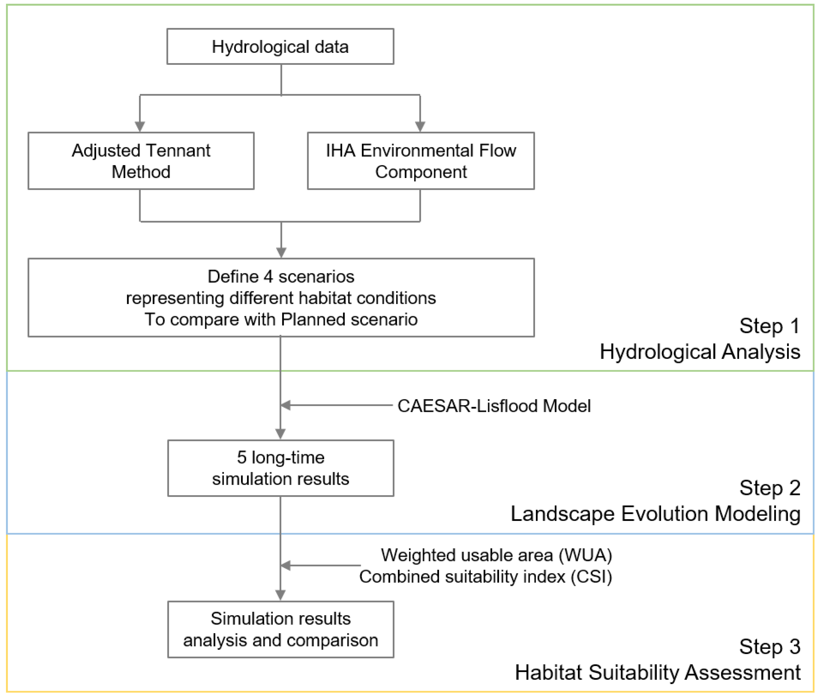
We conducted a three-step sequence of hydrological analysis, landscape evolution modeling, and habitat suitability assessment (
Figure 1) to explore the ecological ramifications of different flow scenarios for the lower Yongding River. First, we used the Indicators of Hydrologic Alteration (IHA) version 7.1 [
37] and the adjusted Tennant method [
38] to understand the historical flow regime and calculate various environmental flow discharges. Second, we applied the CAESAR-LISFLOOD-FP model version 1.9j to simulate long-term (i.e., ten years) landscape evolution under four environmental flow scenarios identified from step 1 and compared them with the flow replenishment plan proposed by the Beijing Water Science and Technology Institute (BWSTI). Finally, we used the Combined Suitability Index (CSI) and Weighted Usable Area (WUA) [
39] method to assess the amount and distribution of suitable fish habitat and compare the ecological effects of all five flow scenarios.
IHA is a software program developed by Nature Conservancy in the 1990s that assesses 67 ecologically relevant hydrological parameters. It is one of the most commonly applied methods to help understand the hydrologic and ecological impacts of various disturbances [
40].
The Tennant method developed in the 1970s is a broadly applied ecological flow assessment (EFA) method that uses predetermined percentages of average annual flow (AAF) as ecological flow criteria [
41]. As one of the oldest hydrological approaches for EFA, it does not require extensive data and is of lower complexity than other more sophisticated approaches, such as the hydraulic, habitat simulation and holistic approaches [
25]. However, because the Lower Yongding River had remained dry for four decades and flow replenishment had only occurred for two and a half years by November 2021, with limited ongoing monitoring, the severe shortages of hydrological, hydraulic, and ecological data precluded the use of more complex EFA approaches. Additionally, previous research on the upstream valley section deemed the EFs assessed by the Tenant method appropriate by comparing them with six other hydrological and hydraulic methods, including the low flow index, Texas Method [
42], Q
90 and Q
50 of flow duration curve, Wetted-Perimeter method, and the R2Cross method [
43].
The CAESAR-LISFLOOD-FP model is an integration of the well-established CAESAR (Cellular Automaton Evolutionary Slope and River) Landscape Evolution Model developed in the early 2000s [
44,
45] and the LISFLOOD-FP hydraulic model [
46]. We selected C-L due to its advanced abilities and computational efficiency in simulating large-scale river corridors (1–100 km
2) over a long period (1–100 years) [
34]. It can simulate both lateral channel changes and sediment erosion and deposition processes in catchments and reaches over varying spatial and temporal scales. Additionally, C-L can efficiently incorporate flow regimes at up to daily resolution instead of a steady discharge. Its ability to estimate erosion and deposition also allows the direct application of widely adopted habitat assessment methods such as the Combined Suitability Index (CSI) method introduced below.
The CSI method was developed in the 1980s and has been widely applied to quantify the suitability of a given habitat for a species of interest, based on habitat suitability curves (HSCs) that relate physical habitat characteristics to species’ preferences [
39,
47]. The weighted usable area (WUA) is an area-weighted habitat suitability index indicative of instream habitat availability for the chosen species [
48]. CSI and WUA were chosen due to the severe lack of baseline ecological data.
Below we introduce the area of interest and elaborate on the specific methods applied at each step.
2.1. Study Area
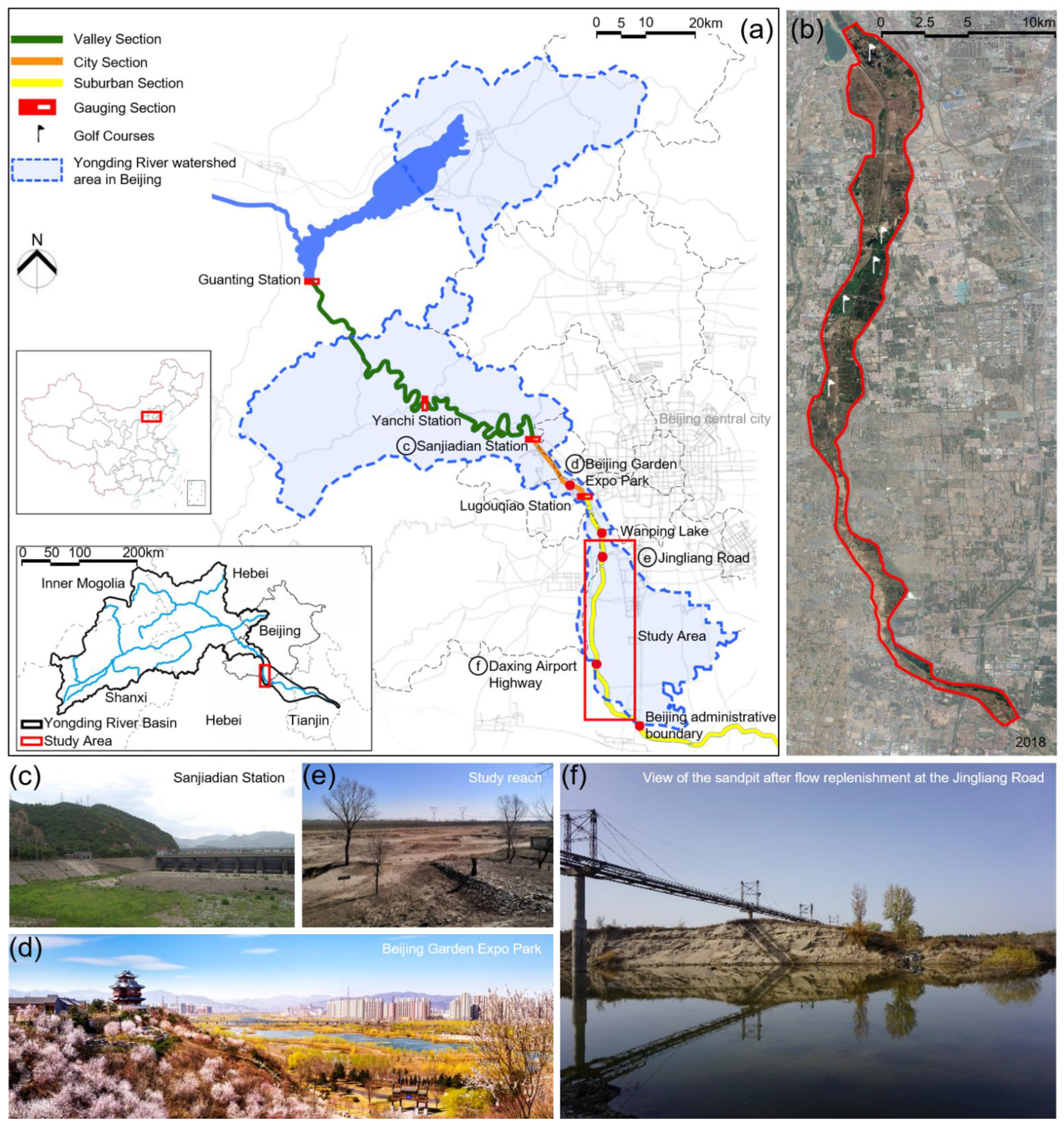
Our study area is a 48km-long downstream segment of the Yongding River (112–117°45′ E, 39–41°20′ N) (
Figure 2). The entire YDR is 747 km long, with a drainage area of 47,016 km
2. It flows from the west to the east across three provinces into Beijing at the Guanting Reservoir (Beijing’s largest reservoir built in 1951) and drains into the Bohai Bay in Tianjin (
Figure 2). The YDRB is in a semi-humid and semi-arid climate transition zone, with annual average temperatures ranging between 5.1–7.1 °C and annual average precipitation of ~400 mm. The climate features a strong seasonality, with 70–80% of its rainfall occurring in summer from June to August.
The Yongding River Beijing segment is 170 km long, draining 3168 km
2 of land and accounting for 6.7% of YDRB. This 170-km segment can be divided into three sections (
Figure 2a): (1) the valley section (91.2 km) from Guanting Reservoir to Sanjiadian gauging station; (2) the city section (18.4 km) from Sanjiadian to Lugouqiao gauging station, and (3) the suburban section (59.8 km) from Lugouqiao to Beijing’s south administrative boundary. For the valley section, long-standing agricultural practices and reservoir operations since 1951 have been the primary factors influencing the river channel. For the city and suburban sections, reduced streamflow, groundwater depletion, limited precipitation, and loss of stormwater to drainage networks have led to the channel becoming perennially dry since the 1980s (
Figure 2c,d) [
49]. Subsequently, agricultural uses expanded, and new recreational uses occurred within or adjacent to the channel. For example, during 2005–2008, certain riverine villages took advantage of legal loopholes and rented their properties to developers, causing at least five golf courses to be built entirely or partially within the channel [
50].
In 2009, the Beijing government began to revitalize the city section and, by 2014, constructed five in-channel public parks through various strategies such as sewage interception, flow replenishment, seepage control, and reuse of reclaimed water [
51]. For example, the Beijing Garden Expo Park at the south end of this section, the 2013 Garden Expo site, transformed a 30-m-deep sandpit into a 35-hectare wetland and 69 sub-gardens that showcased international and national garden cultures.
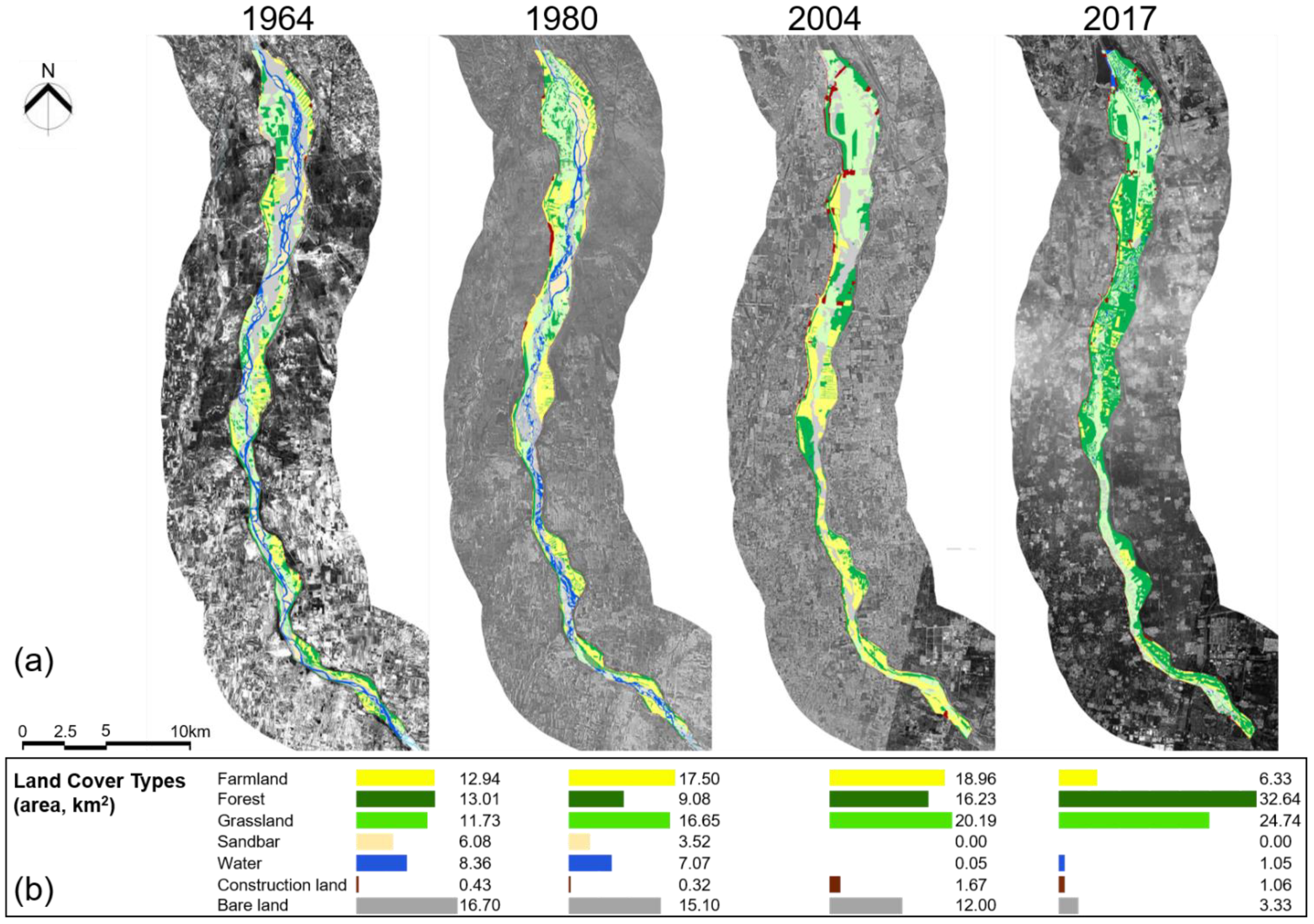
Our chosen study reach is the 48km-long, 69.30-km
2 lower part of the suburban section, extending from Wanping Lake to Beijing’s southern border (
Figure 2). Since the reach dried up in the 1980s, in-channel agricultural uses first increased, but then decreased after 2005 due to riparian greening efforts that have continued to date. As noted above, partially forested golf courses were built during 2005–2008 in the name of greening, increasing forests and lawns (
Figure 3). The channel remained dry until 2019. As the study reach became one of the critical ecological restoration areas of the General Plan mentioned in
Section 1, exploratory flow replenishment began in 2019. A total of 132 million m
3 (Sanjiadian Station) of water was released in 2019, lasting for 54 days from April to June, primarily at a rate of 10 m
3/s and occasionally at 20 m
3/s (for 7 days during 5/18–5/24), 30 m
3/s (for 4 days during 5/25–5/28), and 60 m
3/s (for 1 day on 6/6). In 2020, flow release occurred for 24 days from April to May, totaling 210 million m
3. Two high flow events up to the 3-year return period flow (380 m
3/s) were released on 5/8 and 5/14, each for a full day, while the average discharge was maintained at 70 m
3/s for all other times.
The dire ecological conditions before flow replenishment, representativeness of drying urban streams in northern China, and ongoing rehabilitation efforts make Yongding River a natural laboratory for experimenting with flow restoration strategies to achieve long-term ecological enhancement. Although field monitoring is underway to investigate the ecological effects of early replenishment, modeling approaches are urgently needed to inform future flow distribution before monitoring outcomes are available.
2.2. Characterizing Historical Flow Regime
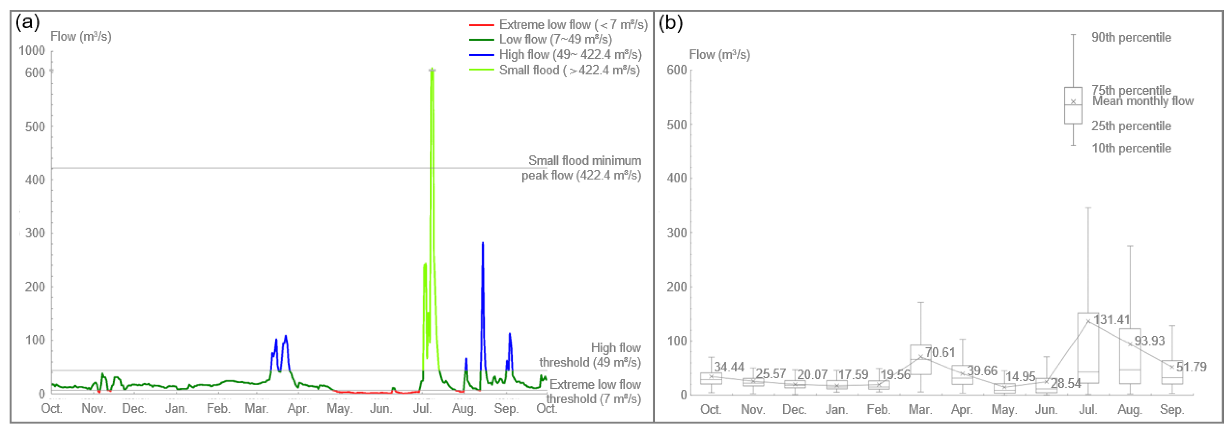
To understand the historical flow regime under which the aquatic ecosystem had evolved, we first used IHA to quantify critical environmental flow components (EFC). IHA is a software program that assesses 67 ecologically relevant hydrological parameters to help understand the hydrologic and ecological impacts of various disturbances [
37]. Because the flow regime became heavily regulated after the Guanting Reservoir was built in 1951, we selected the earliest streamflow records from 1920–1951 (water year, WY) as the reference flow regime. More specifically, after examining all the flow data available at the four gauging stations, i.e., Guanting, Yanchi, Sanjiadian, and Lugouqiao (
Figure 2), we selected the Sanjiadian Station (116°06′ E, 39°58′ N) with the highest data integrity as the primary data source. Daily flow records for WY 1920–1949 and monthly records for WY 1950–1951 were subject to IHA to calculate five EFC parameters, including extreme low flows, low flows, high flow pulses, small floods, and large floods (
Figure 4a).
The IHA calculation indicated that the range of extreme low flows was 0–7 m
3/s, low flow was 7–49 m
3/s, high flow was 49–422.4 m
3/s, small floods was 422.4–2160 m
3/s, and large flood was >2160 m
3/s. Using WY 1931 as an example,
Figure 4a illustrated a representative annual streamflow regime featured by a distinct seasonality. Historically, the long low-flow season typically lasted from September to March, with subsequent brief spring high-flow events in March. The low flows then decreased into extreme low flows until the summer storms arrived. Pulses of massive floods and high flows, intermingled with low flows in between, featured the summer months of July and August. The 1920–1951 historical records also showed that high flows occurred in March, July, and August, about twice a year on average, whereas small floods mainly occurred in July and August once every two years. In wetter years, when small floods occurred, the high-flow season could start as early as June and last until the end of September.
2.3. Identifying Flow Scenarios
To explore how various environmental flow scenarios may affect long-term channel geomorphology, we obtained the flow replenishment plan (aka “PLAN”) developed by BWSTI [
52] and compared it with four continuous flow scenarios (S1–S4) developed with the modified Tennant method [
38] (
Table 1).
Specifically, BWSTI’s PLAN proposes a total annual replenishment volume of 260 million m
3 (at Sanjiadian). It sets the monthly average flows to 15 m
3/s in March–May, 7 m
3/s in June–September, and 11 m
3/s in October, and proposes two high-flow events in spring and autumn with a discharge of 60 m
3/s or higher for 3–5 days [
19].
The four continuous flow scenarios we developed with the modified Tennant method represent four different habitat conditions: optimum, excellent, fair, and poor. Because the constant use of the mean annual flow (MAF) in the original Tennant method [
41] cannot reflect the substantial monthly flow variability of the Yongding River, we replaced the MAF with mean monthly flows (MMFs) [
38] calculated with Sanjiadian’s 1920–1951 flow records (
Figure 4b). Monthly environmental flows were then calculated based on the predetermined percentages of MMFs for winter (October–March) and summer (April–September) [
41] to represent the four specified habitat conditions (
Table 1). The total annual flow volumes estimated for historical conditions, those actually released in 2019 and 2020, proposed by PLAN, and required for the other four flow scenarios are listed in
Table 2.
2.4. Modeling Landscape Evolution with CAESAR-Lisflood
As mentioned above, the C-L model integrates the CAESAR Landscape Evolution Model [
44,
45] and the LISFLOOD-FP hydraulic model [
46]. CAESAR simulates landscape changes by routing water and sediments through a grid of cells and updating cell elevations based on calculations of erosion and deposition of each cell [
44,
45]. It does so by integrating four sub-models, i.e., a hydrological model, the flow model, fluvial erosion and deposition, and slope processes. The LISFLOOD-FP model is a raster-based low-complexity hydraulic model, which simplifies the computation by decoupling flows in the x and y directions and treating the 2D problem as a series of 1D calculations through the cell face boundaries [
46]. In C-L, the flow is simulated exclusively by LISFLOOD-FP.
C-L can be run in two modes, catchment and reach. The catchment mode has a single water influx, the rainfall, while the reach mode allows water and sediment to enter from one or more locations of the reach. The required inputs of C-L include a Digital Elevation Model (DEM), sediment grain size distribution, flow influx (reach mode), and Manning’s
n roughness coefficients throughout the study area. Major model outputs include bed elevation, flow depth, and velocity for each cell at each timestep, sediment grain size distribution, and net erosion and deposition for the entire study area [
44].
To set up the C-L model, we first used ArcMap to process 51,774 point elevations measured in 2016 and generate a DEM for terrain representation. Due to the limits of C-L’s computational capacity, a maximum of 1000 × 1000 grids is allowed for the entire modeling area. Therefore, we used 50 × 50 m as the DEM resolution that resulted in a total of 842 × 219 grids. Echoing other studies that used the same resolution [
54,
55], we considered 50 × 50 m appropriate for our primary focus of exploring the long-term evolution of the study reach. To simulate sediment transport, we used the grain size distribution data supplied by BWSTI based on their field measurements in 2019. Besides, a spatially explicit Manning’s
n roughness coefficients table was developed based on existing vegetation conditions to account for the effects of vegetation on fluvial processes. Test runs indicated that the model required 175–210 days to spin up, so the calibration process below focused on examining model outputs after this initial period.
Due to the significant modification to channel morphology since the 1980s and the absence of detailed historical topographical data, we used aerial photographs in June 2020 after the flow replenishment to calibrate the C-L model (
Figure 2f). Specifically, we used the 2019 DEM and the actual replenishment discharges as the model input and compared the simulated wetted areas with those interpreted from the 2020 aerial photographs. The Producer’s Accuracy [
56,
57] was then used to evaluate how frequently the simulated wetted areas were correctly shown on the classified map. Through iterative calibration and verification processes, nine critical factors recommended by Ziliani et al. [
58], including lateral erosion rate, number of passes for edge smoothing filter, max erode limit, min time step, min Q for depth calculation, water depth above which erosion can happen, suspended sediment load, bedload solid transport formula, and vegetation critic shear (see specific parameter settings in
Table S1, Supplementary Material), were set at values appropriate for the specific spatial and temporal resolutions of this study. Like many other fluvial geomorphic studies, the calibration was qualitative in nature due to severe data limitations but remained critical to improving the model accuracy. The final Producer’s Accuracy value was 87%, exceeding the commonly recommended 85% target [
59,
60]. Besides, during calibration runs, the model spin-up time stayed within 175–210 days, so we used 210 days as the final spin-up period.
The five flow scenarios identified in
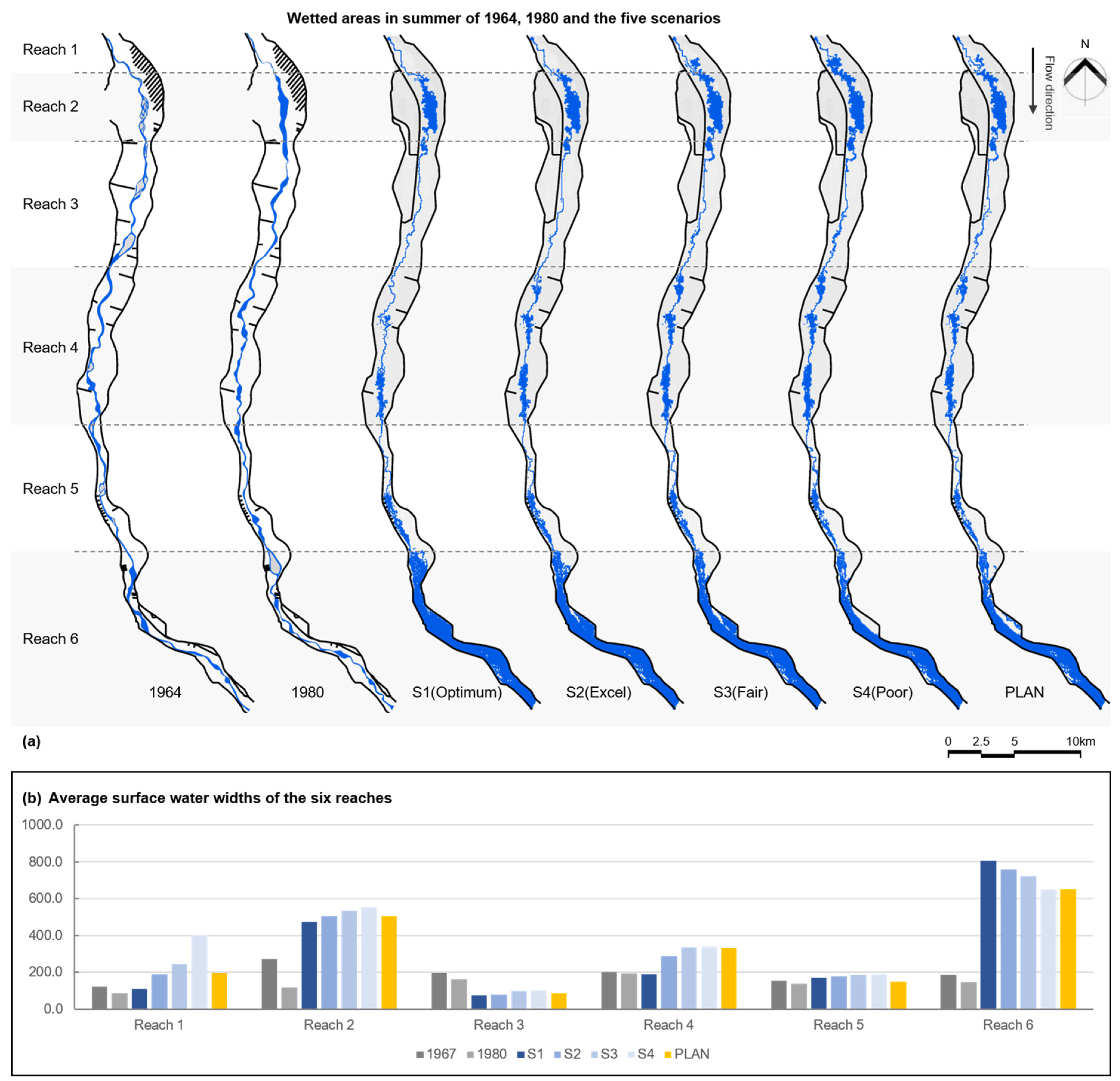
Section 2.3 were subsequently simulated in C-L for ten years after the 210-day spin-up period. Monthly outputs of flow velocities and water depths from the 10th year, bed level changes, and net sediment transport volume at the end of the run were directly exported from C-L. Monthly wetted areas, surface water widths, and elevations were calculated from water depths and bed elevation changes. All the above parameters were then compared among the five scenarios to synthesize the range of channel geomorphic changes. Additionally, surface water widths were compared to those estimated from the 1964 and 1980 aerial photos to understand how the physical channel forms under the flow scenarios compared to historic conditions. For ease of communication, the study area was divided into six reaches (1–6) based on the locations of bridges.
2.5. Habitat Assessment
As previously mentioned, we adopted the classical indicators of the Combined Suitability Index (CSI) and Weighted Usable Area (WUA) for habitat assessment due to the lack of baseline ecological data [
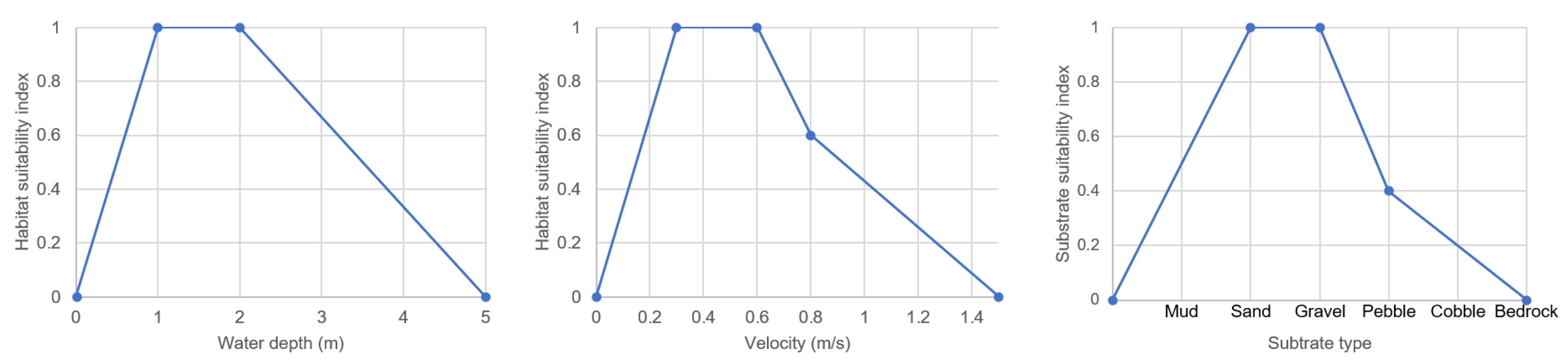
39]. The selection of species of interest was based on a literature review. Additionally, we calculated the Hydraulic Habitat Suitability Index (HHS) to eliminate the size effect of different wetted areas. We specify the methods in detail as follows.
Based on habitat suitability curves that use water depth, velocity, and channel index conditions (substrate and cover) as the primary physical characteristics of stream habitats, we use the formula below to calculate the CSI of a given cell. Water depths and flow velocities are direct outputs of C-L, and
Si has a constant value of 1 in our case due to the substrate being sand. CSI varies between 0~1, with 0 representing unsuitable and 1 most suitable for the given species [
61]. CSI values between 0.6–1.0 can be classified as high suitability, 0.3–0.6 as medium suitability, and 0.1–0.3 as low suitability [
62].
where:
Vi = suitability associated with velocity in cell
i;
Di = suitability associated with depth in cell i;
Si = suitability associated with channel index in cell i.
Because the study reach remained perennially dry between the 1980s and 2019, we relied on reviewing literature and historical records to select the species of interest. According to Zhou [
63], who compared historical records with a 2016 survey, the dominant fish species of the Yongding River Beijing segment, both historically and in the recent past, belong to the
Cyprinidae family, which accounts for 50% of the total number of fish species. Specifically,
Carassius auratus is the most frequently occurring species for the entire Beijing segment, while
Opsariichthys bidens and
Hemiculter leucisculus are also common in the valley and city/suburban sections, respectively. All three species are native to the region, with
Carassius auratus and
Hemiculter leucisculus being highly tolerant of urbanized conditions. Due to the absence of published habitat suitability curves for
Opsariichthys bidens and
Hemiculter leucisculus, we selected
Carassius auratus as the indicator species and used suitability curves developed by Li et al. [
64] (
Figure 5) to calculate CSI for each cell. It should be noted that the channel’s perennial dry conditions during the past four decades precluded the development of more accurate curves based on local field surveys. For the same reason, restoring habitat for dominant fish fishes is in itself an extraordinary challenge with ~560 reservoirs, numerous dams, and ~160 pollution discharge points in the YDRB [
63]. Therefore, we consider the above methods of selecting indicator species and suitability curves appropriate for the purpose of this study.
Building upon the calculations of CSI above, the weighted usable area (WUA), i.e., the area-weighted habitat suitability index [
48], is calculated as:
where:
is the surface area of cell
i, and
is the composite suitability of cell i.
Once WUA is determined, the hydraulic habitat suitability index (HHS) is computed by dividing WUA by the total wetted area [
62], eliminating the size effect of different wetted areas under various flow scenarios. HHS varies from 0 to 1.
4. Discussion
4.1. Geomorphology and Habitat Suitability Effects of Flow Scenarios
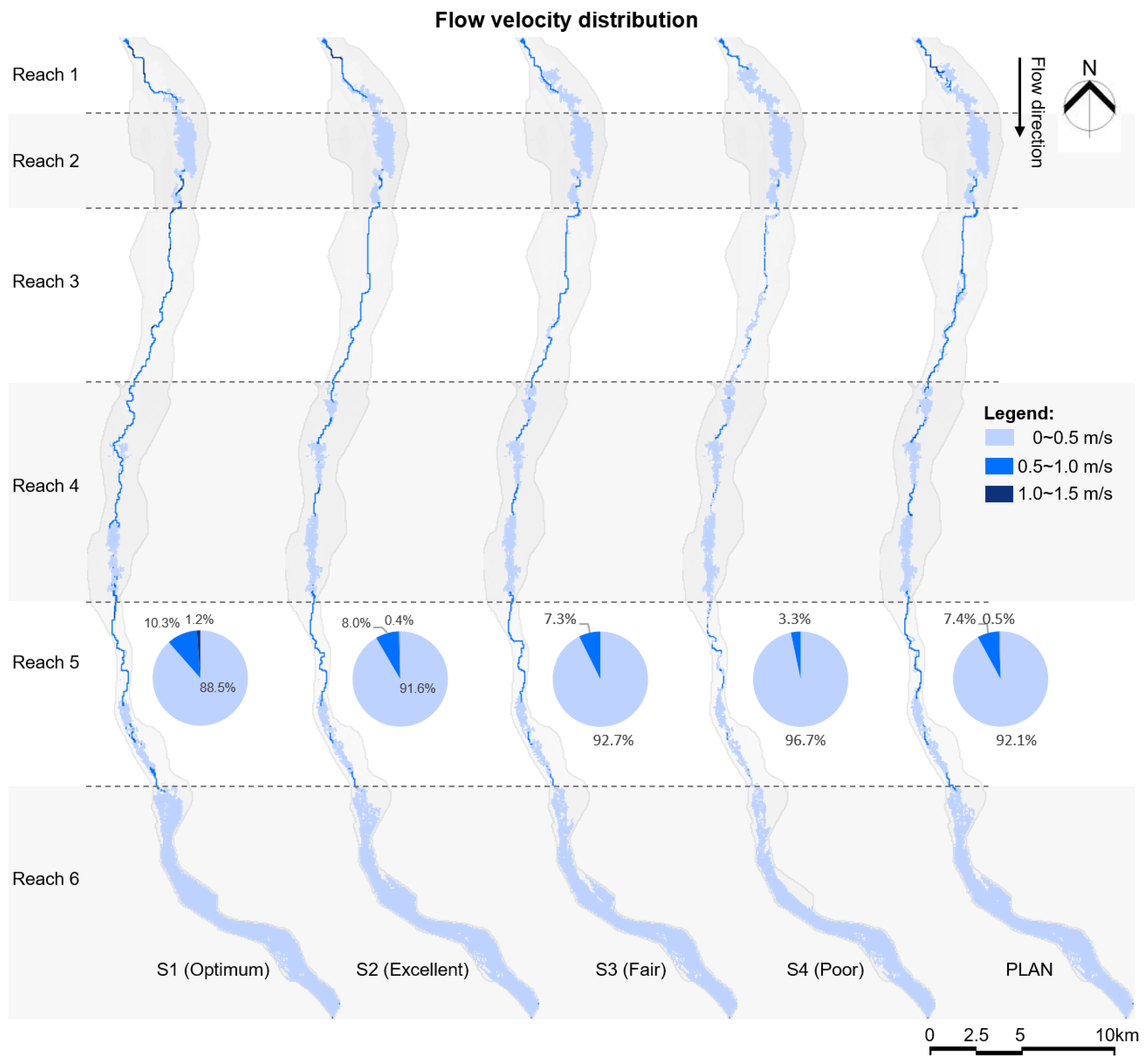
As previously mentioned, a significant widening of most reaches (except Reach 3) was evident in all five future scenarios (average summer surface water width 304.7–339.8 m) in comparison to historical conditions in 1964/1980 (189.3–149.5 m). In particular, the widening of reaches 2 and 6 was primarily due to mining and agricultural activities since the 1980s, whereas the narrowing of Reach 3 can be attributed to flow restriction by riparian tree planting during 2005–2008.
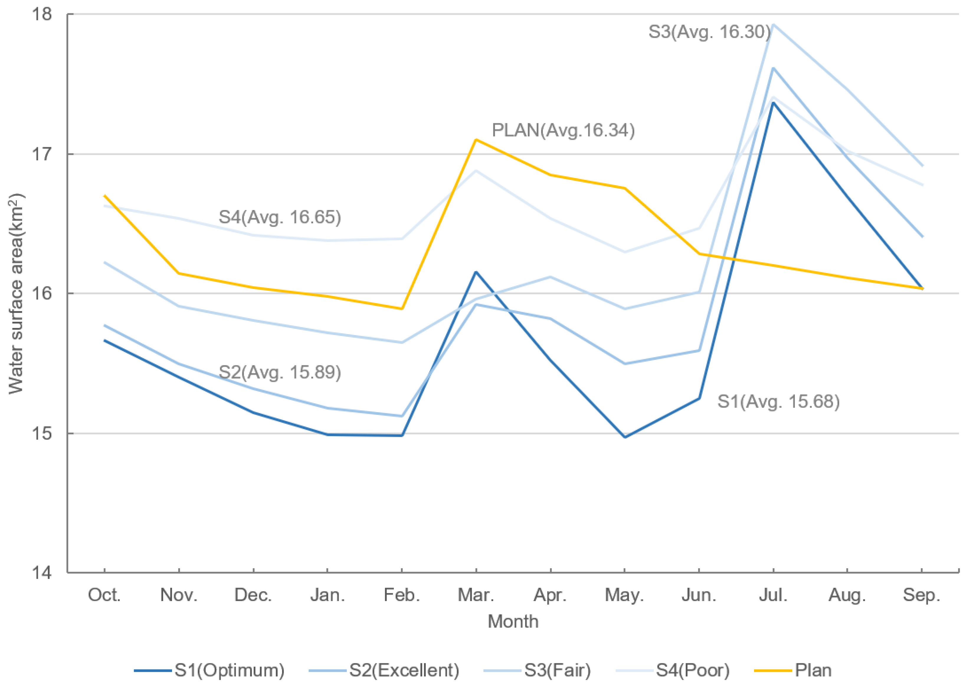
The five flow scenarios showed overall small differences in monthly average wetted area, average surface water width in summer, water depth and flow velocity distributions, and bed level changes. All scenarios had comparable average wetted areas (i.e., 15.68–16.65 km
2,
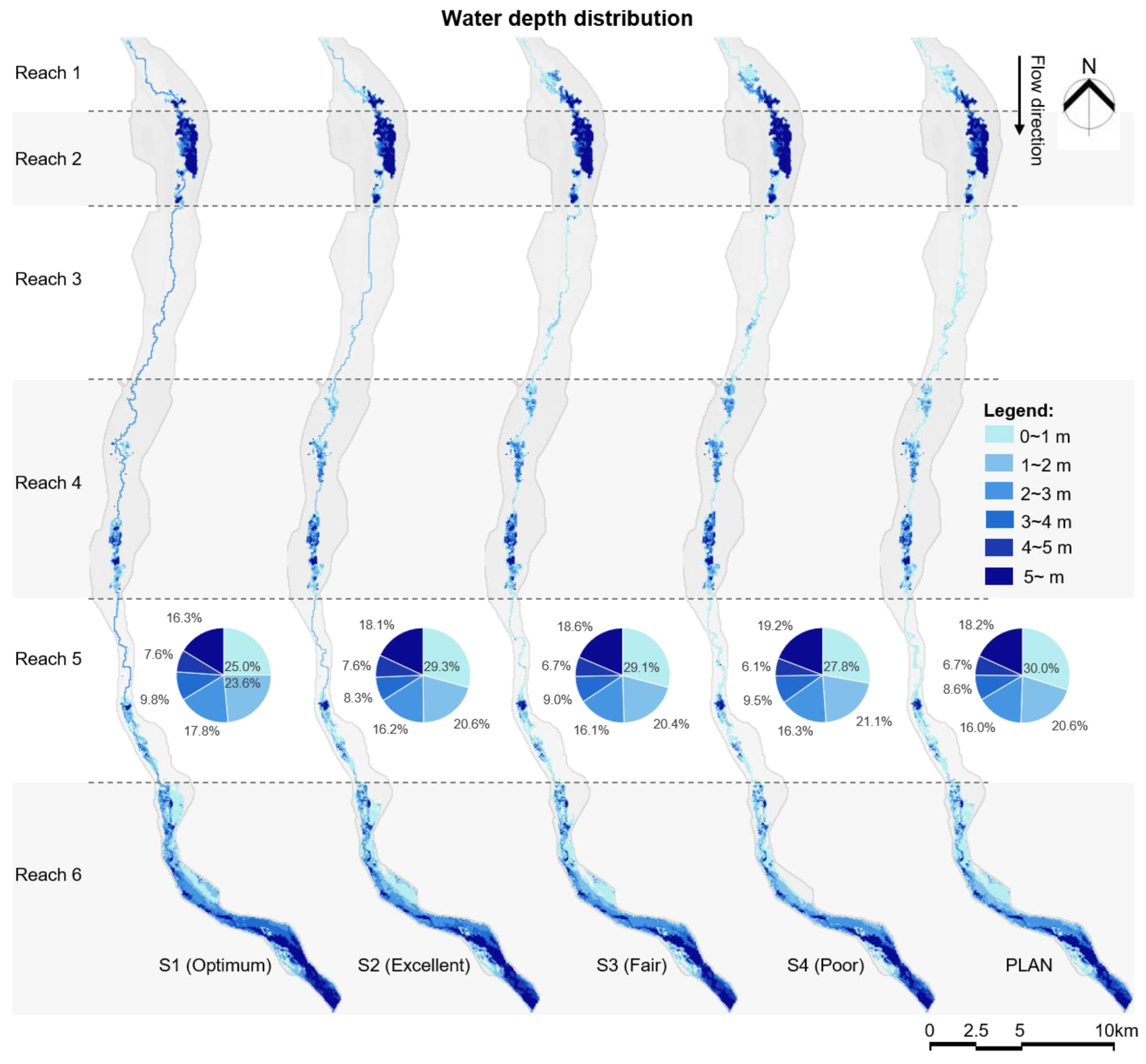
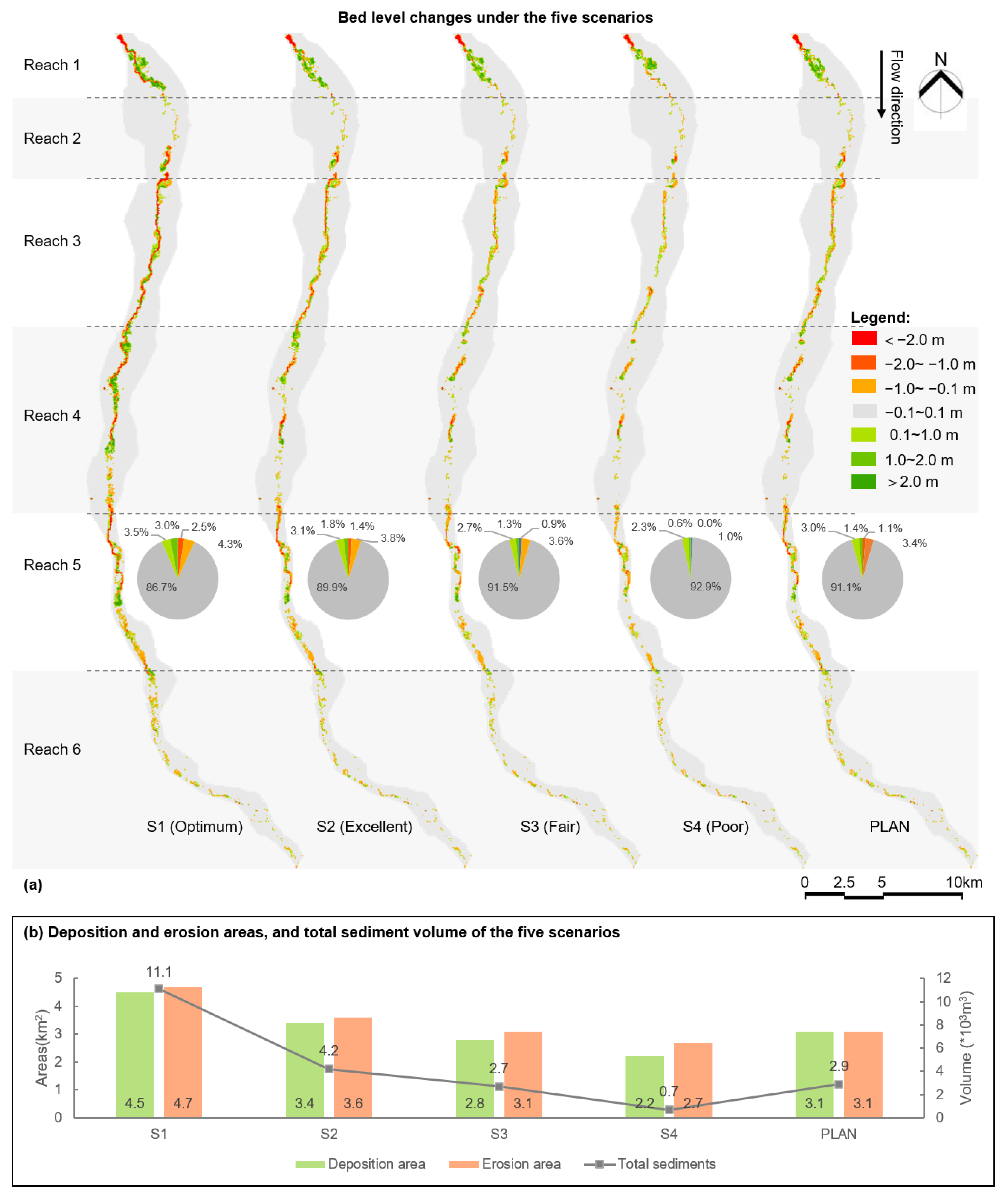
Table S2), summer average surface water width (304.7–339.8 m), water depth (averaged depth ~2.5 m), flow velocity distributions (e.g., 98.8–99.5% occurrences for velocity < 1 m/s), and bed elevation changes (86.8–92.9% change within −0.1–+0.1 m).
However, when individual reaches were examined, cross-scenario variations were more pronounced. For example, the three reaches of 1, 3, and 4 were where morphological differences were the most prominent across the five future scenarios (
Figure 8 and
Figure 10 depth/bed level changes). Within these reaches, a distinct channel formed under high-flow scenarios (S1) while shallow water remained the primary habitat type under other lower-flow scenarios. On the contrary, reaches 2 and 6 presented minor changes (
Figure 10a), indicating the limited effectiveness of flows in reshaping these reaches.
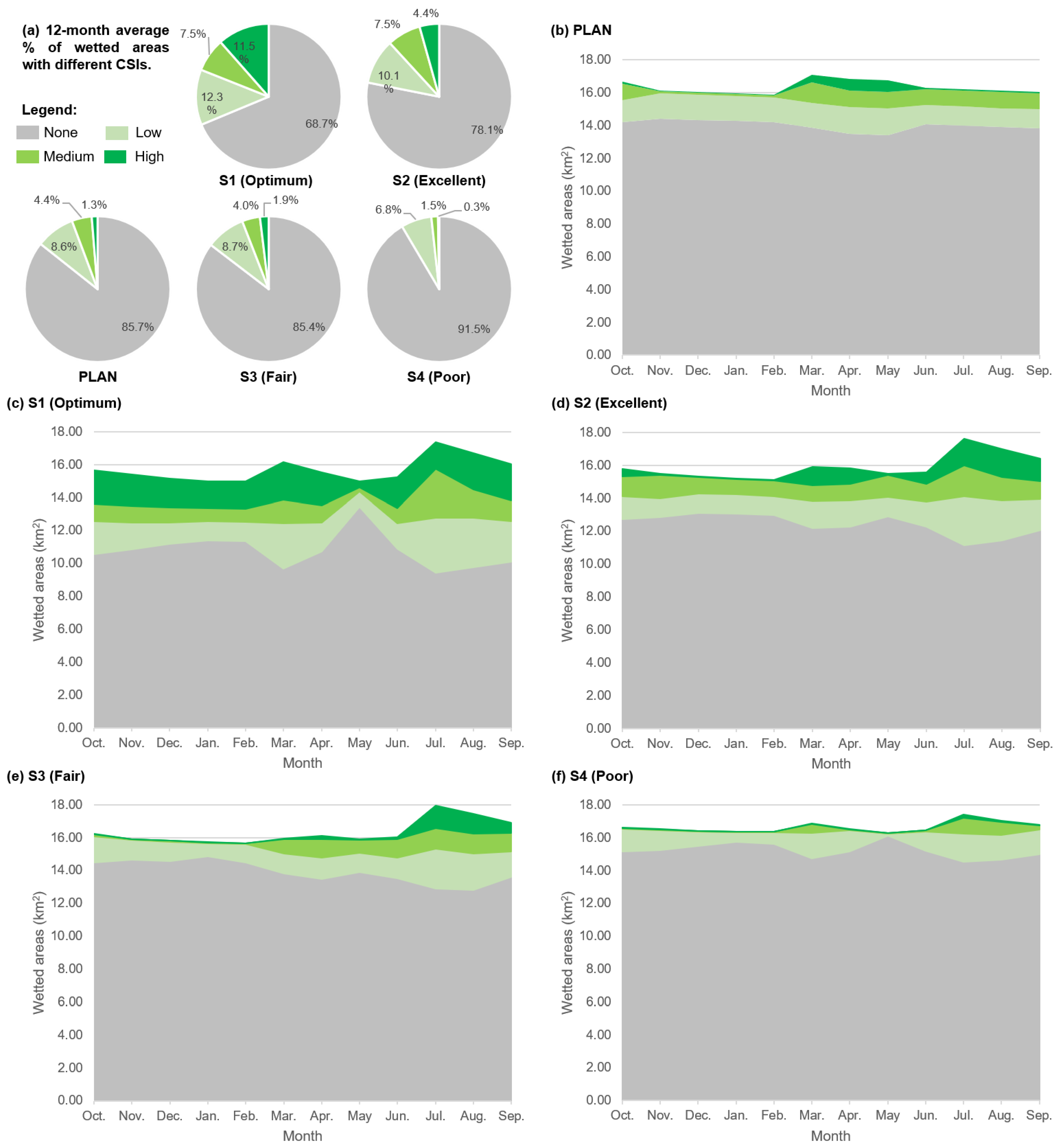
With respect to habitat suitability for
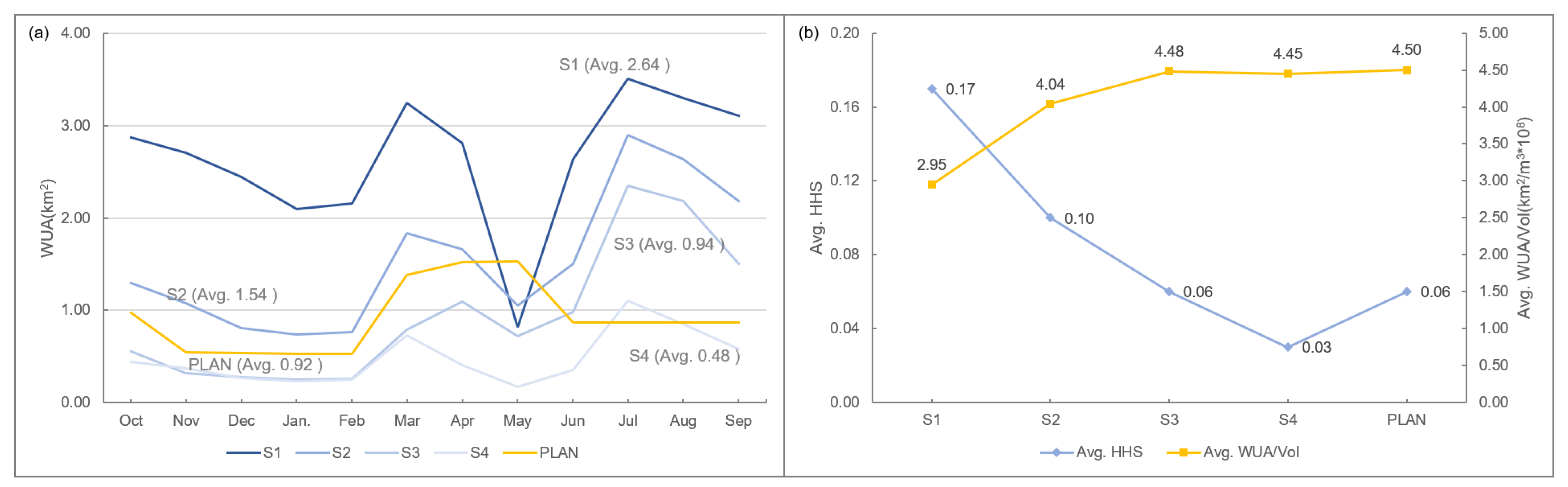
Carassius auratus, higher flows generally led to larger and more evenly distributed habitat areas with high/medium CSIs. However, higher flows in S1 appeared to have generated limited payback in habitat creation, as suggested by its lowest WUA/flow volume value. On the contrary, while PLAN had a small flow volume, its highest WUA/flow volume value and comparable WUA and HHS to S3 send an optimistic message that low monthly flows combined with high flow events can be a viable option when upstream water sources are limited. We will elaborate more on the effects of high flows in
Section 4.3 below.
4.2. Legacy Channel Alterations Affect Flow Replenishment Effectiveness
The limited morphological effects above indicated that extensive, historic geomorphic modifications could have played a significant role in limiting the ability of the prescribed flow regimes to reshape the channel. Specifically, reaches 2 and 6, the two reaches that have endured sand mining and farming, showed no significant morphological changes under any scenario. In the former, a massive sandpit (900 m in diameter, 23.6 m below its east bank at the lowest point) led to a large, deep pond in all scenarios. In contrast, in the latter, over 20 years of farming created large shallow open water areas in all scenarios. None of the scenarios had currents strong enough to form a distinct channel. Similarly, the habitat suitability indexes remained low for reaches 2 and 6 throughout the year, regardless of the flow scenario (
Figure 13a). Therefore, for heavily modified rivers, flow replenishment alone is not enough to achieve the desired morphological and ecological effects, echoing literature findings that channel form and morphologic complexity can be as important as flow for providing habitat [
65,
66,
67,
68]. Managing for flows purely relative to a historic natural flow regime may be insufficient without the appropriate considerations for the hydraulic and morphological outcomes.
For reaches 2 and 6 at least, the channel structure needs to be restored to a certain degree for environmental flow implementation to effectively influence habitat. For example, restoring the channel structure in these reaches to mimic pre-1980s historical conditions could set the stage for re-establishing the dynamic process–response relationship between the flow regime and its geomorphic and ecological outcomes. However, the new channel design should be based on management objectives and the anticipated future flow and sediment regimes. Additionally, to enhance financial feasibility, bed and bank topography can be carefully modified to create a solution with an in-channel cut-and-fill balance to reduce the cost. For example, the farmland in Reach 6 can be excavated to form a distinct channel, and the cut materials can be utilized to partially fill the sandpit and create a channel connection in Reach 2. Future simulations can be conducted to assess specific channel design scenarios. Again, the revealing of limited ecological benefits due to legacy channel modifications highlights the significance of the landscape evolution modeling approach for evaluating proposed flow regimes and channel designs in heavily modified rivers.
Moreover, social and economic impacts should be assessed in searching for an ideal channel restoration plan. For example, restoring the channel structure in Reach 6′s farmland will inevitably affect farmers’ social and economic well-being. A thorough and thoughtful public participation process can help gain public recognition and support, while strategies such as land swap and monetary compensation could help mitigate adverse financial impacts to the farmers.
4.3. High Flows Effectively Create Habitat
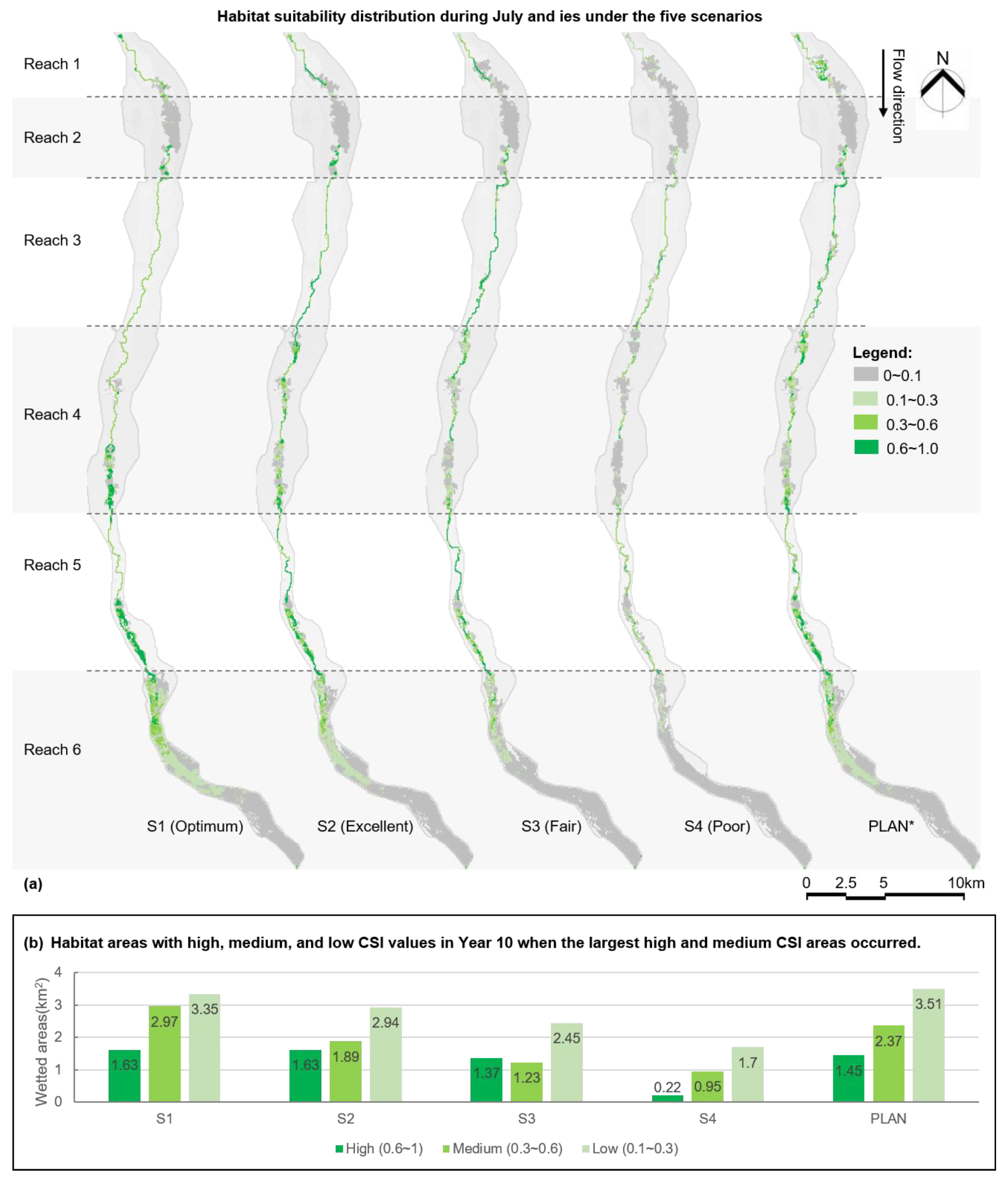
Despite a smaller annual flow replenishment volume, the outperformance of the PLAN scenario over S2 and S3 in multiple geomorphic and habitat suitability metrics confirmed the positive effects of high flows. With 76% (260 of 340 million m
3) of the flow volume of S3, PLAN transported a larger amount of sediments than S3 (2900 vs. 2700 m
3). PLAN also equaled to S3 in the 12-month average HHS (0.06,
Table S7,
Figure 11b) and percentages of high/medium CSI areas (5.7% vs. 5.9%,
Figure 12). Moreover, the 60 m
3/s high-flow event in PLAN created a larger high/medium CSI area than S2 through S4 when their high flows occurred in July (e.g., 3.82 km
2 in PLAN vs. 3.52 km
2 in S2). On the other hand, although it is difficult to use a single metric to compare PLAN with S1, which requires 5.6 times of flow volume (1450 million m
3) as PLAN, a qualitative assessment can be made that S1 may not offer proportional ecological benefits. For example, the 12-month average HHS was 2.8 times higher in S1 than PLAN (0.17 vs. 0.06); the 12-month average % of high/medium CSI areas was 3.3 times higher in S1 than PLAN; the peak high/medium CSI area was only 1.2 times higher in S1 than PLAN. These comparisons highlight the effectiveness of high-flow events in PLAN in shaping the aquatic habitat.
Despite its evident habitat effects, the arbitrarily chosen 60 m
3/s event in PLAN may not be high enough for the channel to regenerate habitat. It was only slightly higher than the high flow threshold (49 m
3/s) but significantly lower than the small flood threshold (422.4 m
3/s) revealed by the previous IHA analysis. Occasional artificial floods, such as two- to five-year return period events (160–820 m
3/s in this case), can be crucial for maintaining sediment and floodplain dynamics [
25]. Future modeling will be necessary to help identify alternative flow regimes that incorporate potentially higher flows (e.g., at a lower frequency) to more effectively create habitat. These alternative flow regimes should be developed within the context of the priority management objectives for the restoration effort.
4.4. Thoughts on Future Directions
Substantial investments are being made to improve the condition of and the diverse social benefits that can be provided by the YDR, specifically in the form of an annual replenishment water volume of 260 million m3 implemented through environmental flow releases. This study assessed the relative improvements that might be achieved through different water allocation scenarios, and more broadly highlights the value of using a landscape perspective and scenario-based approach to help guide future restoration efforts. Of critical importance is the need for any management action to be taken through an integrated water resource management (IWRM) framework, based on clearly articulated restoration objectives that couple efforts of managing flow and sediment regimes and channel structure in the basin.
Adding to the challenge is the uncertainty associated with climate change and resulting precipitation patterns, water availability, and possible flow regimes. As is, the current replenishment volume of 260 million m
3 remains a fraction (~18%) of the historical average annual discharges (1.453 billion m
3) during 1920–1950. Moreover, the current sole reliance on cross-basin transport of water for environmental flow purposes may be highly vulnerable under climatic uncertainty and face fierce competition from other water uses. However, a landscape perspective and strategies developed and advanced through IWRM afford opportunity. For example, water conservation efforts could be adopted in upstream sub-watersheds, especially for the agricultural sector which is the largest water use in the YDRB [
69]. Moreover, substantial potential exists in the reclamation of local greywater and stormwater as additional sources for in-stream flows. For example, research has shown that 75 million m
3 of greywater can be reused to supply the YDR every year [
70], although the potential of stormwater management remains unassessed. Developing an integrated management plan that incorporates basin-wide stormwater management and the distribution and treatment of reclaimed water will be a critical next step to enhance the overall ecological conditions of the entire basin and the benefits it provides society.
Finally, as with other restoration efforts, work to enhance the YDR should include monitoring and be advanced through adaptive management to ensure that investments are returning benefits and improving scientific understanding that can be used to guide future management of this dynamic and heavily modified system. Long-term monitoring studies will require cooperation across many disciplines such as climate science, hydrology, geomorphology, ecology, engineering, and landscape planning and design; while adaptive management will require policymakers and managers to be an integral part of the team to ensure swift management actions can be made in response to monitoring outcomes.
4.5. Study Limitations
With important implications for urban river rehabilitation in water-scarce cities in China, we note several limitations of our study, some of which are not uncommon for similar studies. First, as with others with habitat suitability curves, the evaluation of the scenarios relied on a minimal number of HSCs. That was primarily due to the scarcity of ecological baseline data with extensive ecosystem disturbance since the 1980s. Although using a single set of HSCs to represent one species’ requirements has been common, numerous authors have suggested adopting broadened criteria such as those representing habitat guilds [
71,
72,
73,
74] or multiple indicator species with drastically different seasonal needs [
75]. Future efforts should be made to communicate with regional ecologists to create additional habitat suitability curves or information to test geomorphic and ecological consequences for other species to optimize flow allocations.
Additionally, the computational limitation of C-L does not allow a large number of scenarios to be tested within a short amount of time. Our pilot modeling began to reveal the potential consequences of chosen scenarios but showed a limited capacity to test interventions. As mentioned above, future modeling should continue to evaluate various channel modification scenarios of the mine pits and agricultural field at the minimum. Other flow replenishment scenarios that further incorporate the environmental flow components calculated by IHA should also be tested.
5. Conclusions
By connecting the landscape evolution model CAESAR-Lisflood with the habitat suitability index method, we assessed the morphological outcomes and habitat suitability under five environmental flow scenarios for the highly urbanized Yongding River of Beijing, China. We found that, first, although the five flow scenarios showed minor differences in metrics such as monthly average wetted area, average surface water width in summer, water depth and flow velocity distributions, and bed level changes, cross-scenario variations were more pronounced in specific reaches, where high- instead of low-flow scenarios were able to shape a distinct channel. The lack of physical responses of the other reaches may be attributed to historical channel modifications such as in-stream mining and agriculture. Second, the higher-flow scenarios generally led to larger and more evenly distributed habitat areas with high and medium suitability for Carassius auratus. However, the PLAN scenario with the second smallest total flow volume generated the highest payback in habitat creation, suggesting that low monthly flows combined with high-flow events show promise when upstream water sources are limited. Overall, for heavily modified urban rivers, flow replenishment based on historical monthly average flows alone may not be adequate to generate the desired morphological and ecological effects. Severe historical channel modifications have to be addressed for flow replenishment to take effect, and the potential for high flows of various magnitudes to shape the channel needs to be further explored to inform future environmental flow management.
This study is the first landscape evolution modeling study of a heavily modified urban stream in China to the best of the authors’ knowledge. While this pilot study has various limitations due to severe data and knowledge shortages, it demonstrated the broad applicability of an interdisciplinary modeling framework based on LEMs and habitat suitability assessment. Moreover, it generated both transferable lessons and specific implications for future research and practices for the Yongding River. Enhancing heavily disturbed stream ecosystems in the face of wicked problems such as water scarcity will continue to challenge our planning and design capabilities. Simulations that test alternative restoration strategies should be leveraged in parallel to the field monitoring of ongoing restoration efforts to guide future restoration actions.


