1. Introduction
1.1. Background
Much of the process water from oil sands surface mining operations is recycled and managed in tailing ponds. However, the capacity for storage is approaching unmanageable and unsustainable levels; hence, some release of treated process water into the Athabasca River is anticipated as early as 2025 [
1]. The release of treated process water may pose a risk to aquatic species and to humans who harvest and consume these species, in particular fish. Therefore, effective models to describe the transport and fate of oil sands related substances are required [
2]. These substances can be transported downstream and deposited in Lake Athabasca and the Peace-Athabasca-Delta (PAD); in addition, secondary channels and lakes within the floodplain along the lower river reach may also trap released sediment and associated constituents. An important objective of this research is to determine the fate of such effluent within these features using computer modelling.
1.2. Water-Quality Modelling
The development of complex three-dimensional integrated hydrodynamic, sediment transport, and water quality models has been proposed to characterize the transport and fate of sediment and associated constituents in the lower Athabasca River, advocated by several researchers and government agencies [
2]. However, the implementation of complex modelling frameworks may not be advantageous for many reasons, including cost, the time required to develop the framework, and lengthy model simulation times. Additionally, model complexity can obfuscate rather than elucidate key processes, and both overly complex and overly simple models can have reduced reliability.
We propose using the Water Quality Analysis Simulation Program (WASP) [
3] to develop a model to characterize the fate and transport of sediment and associated constituents within the lower Athabasca River. WASP is a dynamic compartment-modelling program for aquatic systems, including both the water column and the underlying benthos. Its representation of sediment and material kinetics is more sophisticated than other commonly used models [
4]. WASP is a widely used framework for developing site-specific models for simulating toxicant concentrations in surface waters and sediments over a range of complexities and temporal and spatial scales. WASP has an advanced toxicant module that includes representation of a range of solids classes, with individual physical and chemical characteristics. Solids classes can be organic materials (e.g., plankton, algae, detritus) or inorganic (e.g., sand, silt, clay).
1.3. Quasi-Two-Dimensional Modelling
This paper describes a unique quasi-two-dimensional representation of river hydraulics that is particularly suited to the application of the WASP model to accurately represent the configuration of the lower Athabasca River with a high level of computational efficiency. In the current study, we introduce a novel approach to modelling transverse mixing in a river with secondary channels and side lakes to study the water quality along the area of the Athabasca River with extensive oil sands development.
In order to maintain short computational times, a one-dimensional (1D) modelling approach is necessary. However, the transverse mixing along the river requires modelling with at least a two-dimensional (2D) representation, especially since the lengths of complete mixing along this river are relatively long (>100 km). Hence, the use of a quasi-two-dimensional (quasi-2D) approach is proposed, in which flow is simulated in 1D, but in such a way to allow a 2D discretisation of the domain.
Quasi-2D water-quality modelling has been carried out in the past for other applications. For off-channel storage facilities (polders) along the Elbe River in Germany, Lindenschmidt et al. [
5] modelled dissolved oxygen and nutrient dynamics for various flow regimes (low, medium, high (flood) flows). Deposition of sediments and heavy metals in the off-channel storage basins was captured using the quasi-2D method [
6,
7,
8]. The quasi-2D approach has also been used to capture flows between main river channels and their floodplains, in particular through dike breaches [
9] and capping flood peaks using side-channel storage [
10,
11]. Flow between the Mekong River and its delta [
12] and between the Po River and a portion of its floodplain [
13] were simulated using quasi-2D models. Sediment transport was included in a quasi-2D model of the Rhine River’s main channel and floodplain [
14]. In this study, we extend the quasi-2D approach to model transverse mixing in rivers.
1.4. Objectives
The objectives of this study are to:
Develop a quasi-2D modelling approach to characterise transverse mixing of two water streams of different sediment concentrations.
Assess the role of drawing on the output of additional models to complement the implementation of models with different complexity and spatial scale.
As proof of concept of the approach, the sediment transport along the lower Athabasca River was quantified. The model domain includes a secondary channel and side lake connected hydraulically to the river’s main stem.
2. Site Description
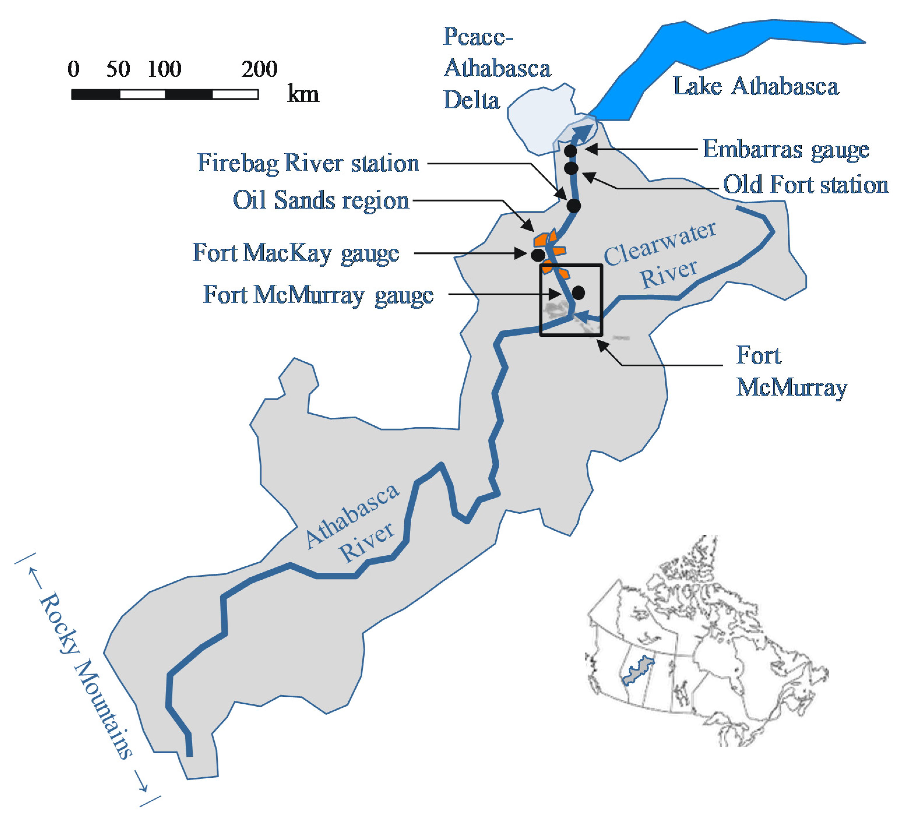
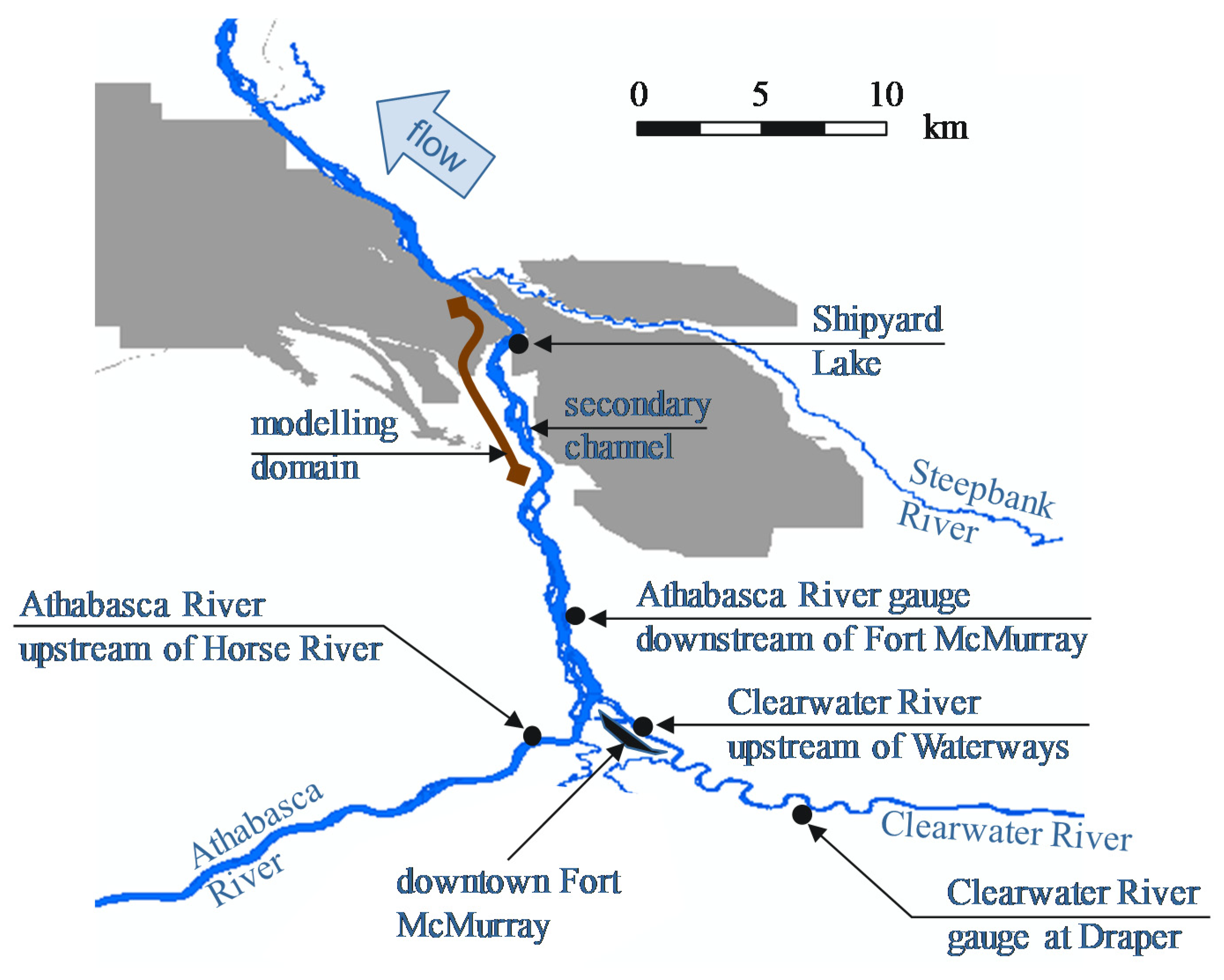
The Athabasca River (see
Figure 1) is a northern river (ice-covered in winter) in western Canada that originates on the eastern slopes of the Rocky Mountains and flows approximately 1500 km in a north-easterly direction to empty into Lake Athabasca. It is the longest unregulated river in Alberta. For the last 80 km, the river flows through the Athabasca Delta. The Athabasca Delta is part of the larger Peace-Athabasca Delta (PAD), which is the largest inland delta in North America. The PAD is an important ecosystem for many aquatic and terrestrial plant and animal species, and the area has been named both a Ramsar and United Nations Educational, Scientific and Cultural Organization (UNESCO) World Heritage site. From a human perspective, the PAD is an important social, cultural and economic entity for many of the Aboriginal communities in the area. Many conservation efforts have been carried out to maintain the ecological integrity of the aquatic and terrestrial systems.
Referring to
Figure 1, the average discharge at the Water Survey of Canada (WSC) gauge at Embarras (gauge 07DD001–Athabasca River at Embarras Airport), which is approximately 80 km upstream of the PAD, is around 850 m
3/s. The total catchment area draining at the same gauge is approximately 156,000 km
2. Much of the basin’s land use consists of forests (89%) with some agricultural lands (8%). The basin is sparsely populated (≈200,000 inhabitants), with the population concentrated in a few urban centres, which release effluent from municipal wastewater treatment plants into the river.
The oil sand region covers a large area of Northern Alberta and has one of the richest deposits of petroleum in the world. For a 65 km stretch of the lower Athabasca River, between Fort McMurray and downstream of Fort MacKay (see
Figure 1), the river flows through the active oil sand surface mines. Much of the oil is extracted through open-pit mining and processed using water from the Athabasca River. Almost 5% of the river’s average flow has been allocated for anthropogenic usage. Although approximately half of that amount is allocated for surface and in situ mining activities, less than 1% is used [
15].
The lower Athabasca River contains many islands, secondary channels, wetlands, and floodplain lakes. Many of these secondary channels freeze to the bottom or have low oxygen levels during winter [
16]. Sediment deposition areas occur downstream of tributaries (confluence bars), in mid-channel bars, in secondary channels and in side lake and wetland areas along the river. During high flow events, substantial amounts of oil sands material can be transported from tributaries into the river to be deposited in these depositional areas. Over time, these areas of high oil sands material are mixed and diluted with water and sediment coming from upstream.
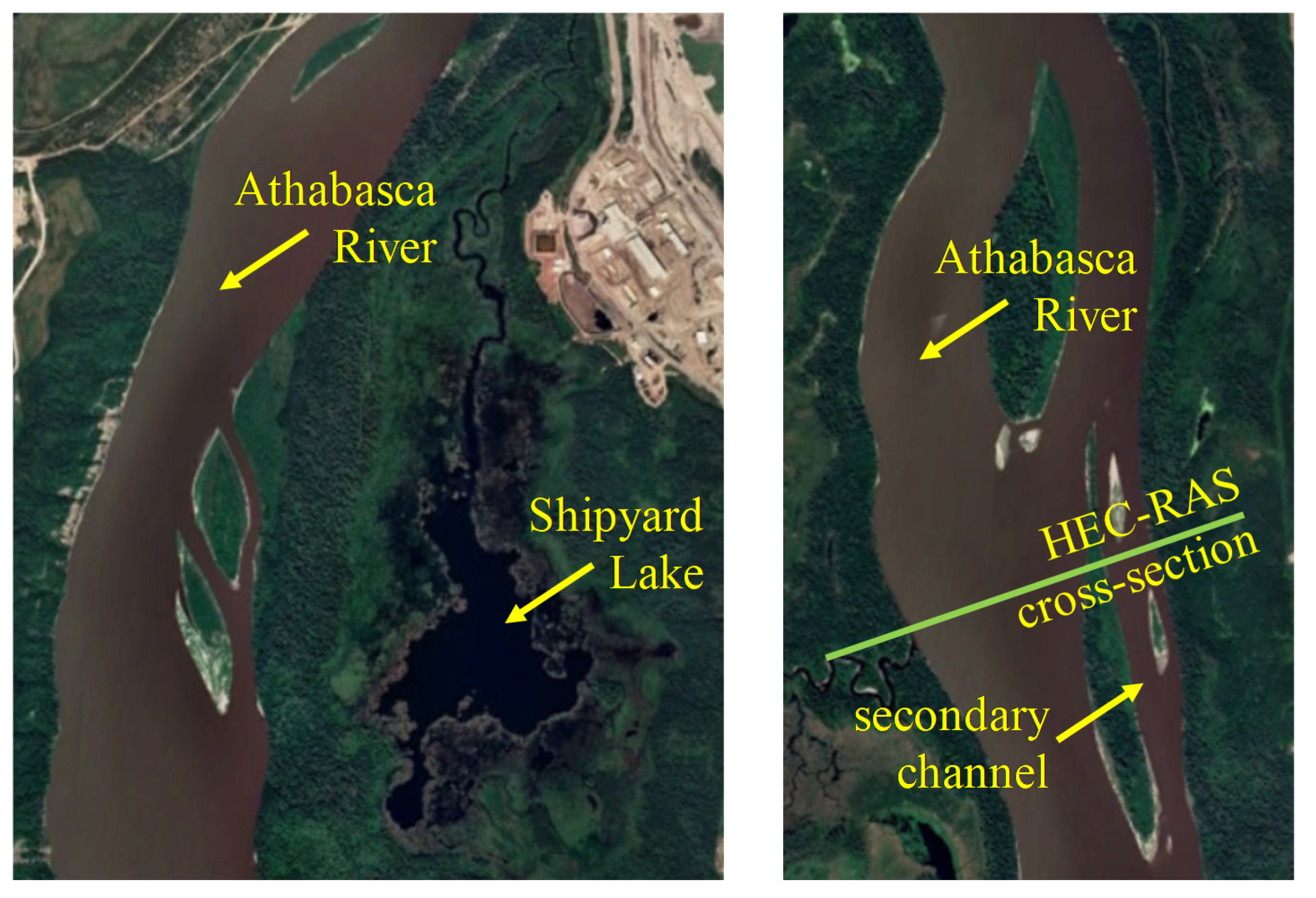
To show proof-of-concept, the domain modelled in this study is only a short stretch of 15 km. It is part of a larger system (>200 km) that is to be modelled in the future, with additional outfalls and sensitive depositional areas (e.g., secondary channels and side lakes). The model domain is indicated in
Figure 2 and was chosen based on the location of proposed outfalls from oilsands operations. One particular side lake of interest in this study is Shipyard Lake, which is located near the Suncor oil facilities on the east side of the Athabasca River and is within the model domain. The lake, shown in
Figure 3, has a surface area of 21.3 ha and a maximum depth of 2.2 m [
17]. It is essentially a large wetland area that is flooded by higher flows from the Athabasca River [
17]. Numerous small creeks feed the lake and water from the Athabasca River flows into Shipyard Lake over a low levee between the watercourse and water body. Flow begins to overflow the levee at an Athabasca River flow of 2800 m
3/s [
18], which corresponds to a water surface elevation of 237.7 m a.s.l. just upstream of the lake [
18]. This corresponds to a water level elevation of approximately 240.1 m a.s.l. at the Athabasca River gauge downstream of Fort McMurray [
19], the location of which is shown in
Figure 2.
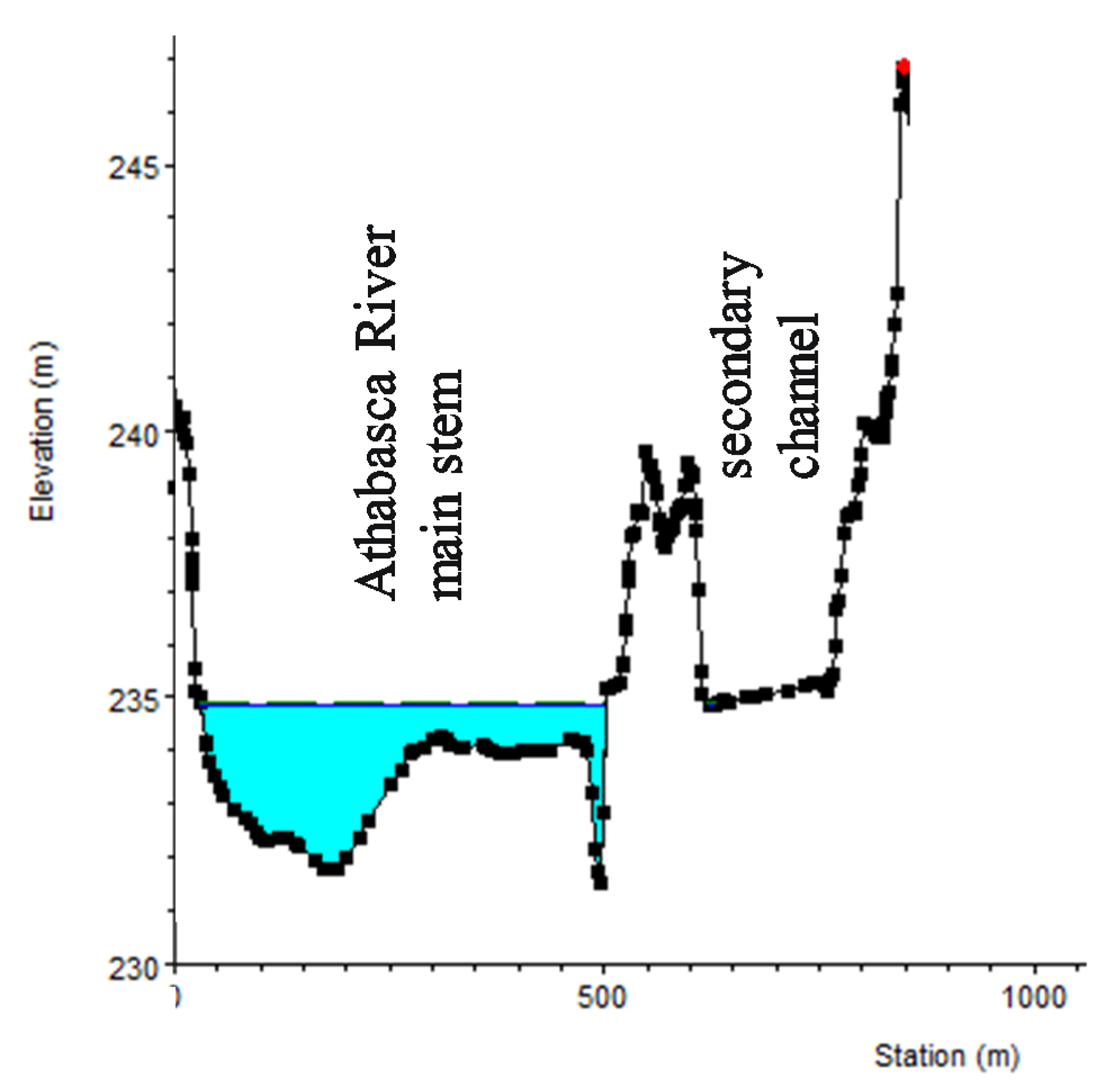
A secondary channel is also included in the model domain, also shown in
Figure 3. Indicated in the figure is the location of a cross-section of the Athabasca River main stem and the secondary channel, which is shown in
Figure 4. Some water does flow into the secondary channel from the Athabasca River at a flow of 600 m
3/s.
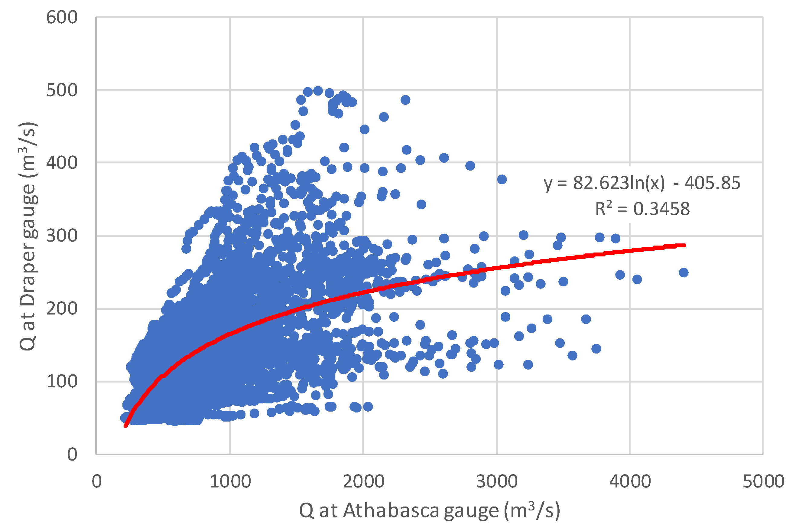
A major tributary of the Athabasca River is the Clearwater River (see
Figure 1 and
Figure 2), which flows from the east into the Athabasca River at Fort McMurray. For an average flow of 600 m
3/s at the gauge on the Athabasca River downstream of Fort McMurray (gauge 07DA001–Athabasca River below Fort McMurray), the average annual flow from the Clearwater River recorded at the Draper gauge (gauge 07CD001–Clearwater River at Draper) is 116 m
3/s and ranges from 30 to 500 m
3/s (see
Figure 5).
Total suspended solids (TSS) data from four stations along the Athabasca River were used in the analysis:
Athabasca River upstream of the Firebag River confluence (Alberta Environment and Park’s long term monitoring station AB07DA0980;
Figure 1)
Old Fort/Devil’s Elbow (Alberta Environment and Park’s long term monitoring station AB07DD0010 (open water) and AB07DD0105 (ice-cover);
Figure 1)
Athabasca River upstream of the Horse River—(Alberta Environment and Park’s long term monitoring station AB07CC0030;
Figure 2)
Clearwater River upstream of Waterways (Alberta Environment and Park’s monitoring station AB07CD0200/210/090 Clearwater River upstream of Waterways;
Figure 2)
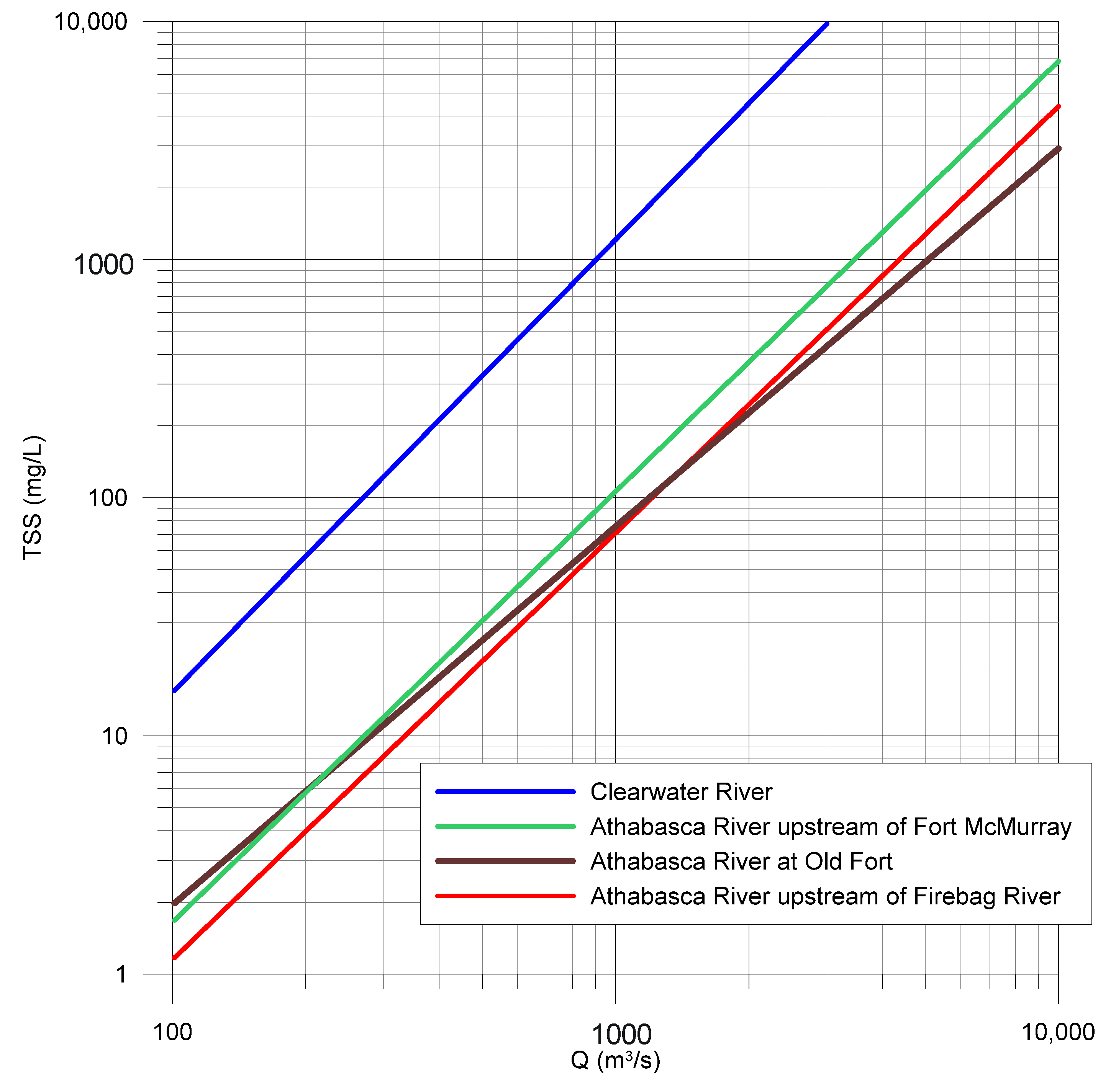
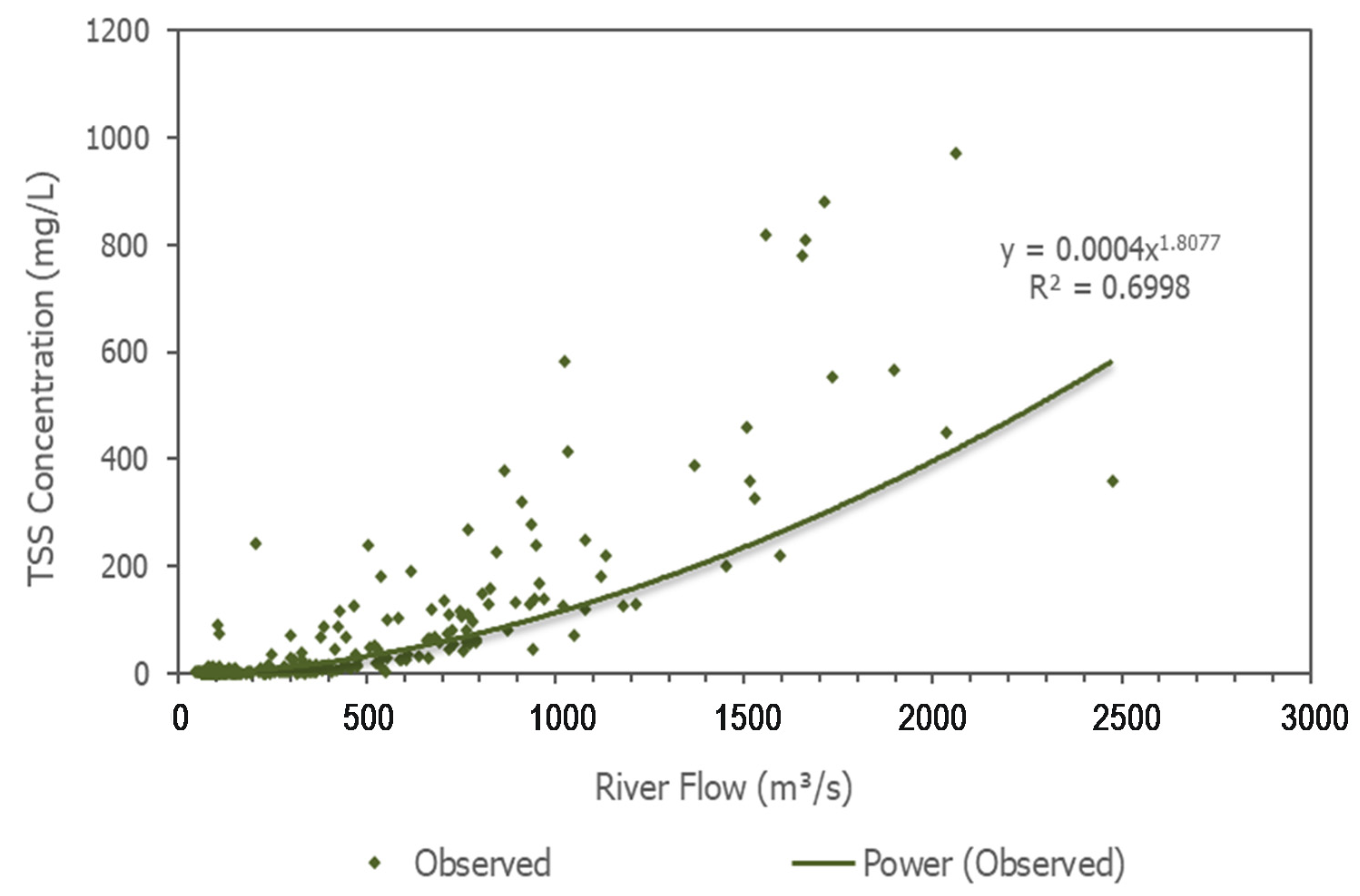
Empirical relationships between TSS concentrations and river discharge are provided in
Appendix A, from which equations were established and are shown in
Figure 6 for a lower flow regime. Sediment transport was simulated only for the 2800 m
3/s flow since, in this scenario, Athabasca River water flows into both the secondary channel and Shipyard Lake. A total flow of 2800 m
3/s at the Athabasca River gauge below Fort McMurray corresponds to a flow of 250 m
3/s for the Clearwater River (from
Figure 5), yielding, through simple subtraction, a flow of 2550 m
3/s at the Athabasca River station upstream of Fort McMurray. From
Figure 6, the TSS concentrations are respectively 575.5 and 86.8 mg/L for the upper Athabasca and Clearwater rivers.
3. Hydraulic Modelling Setup
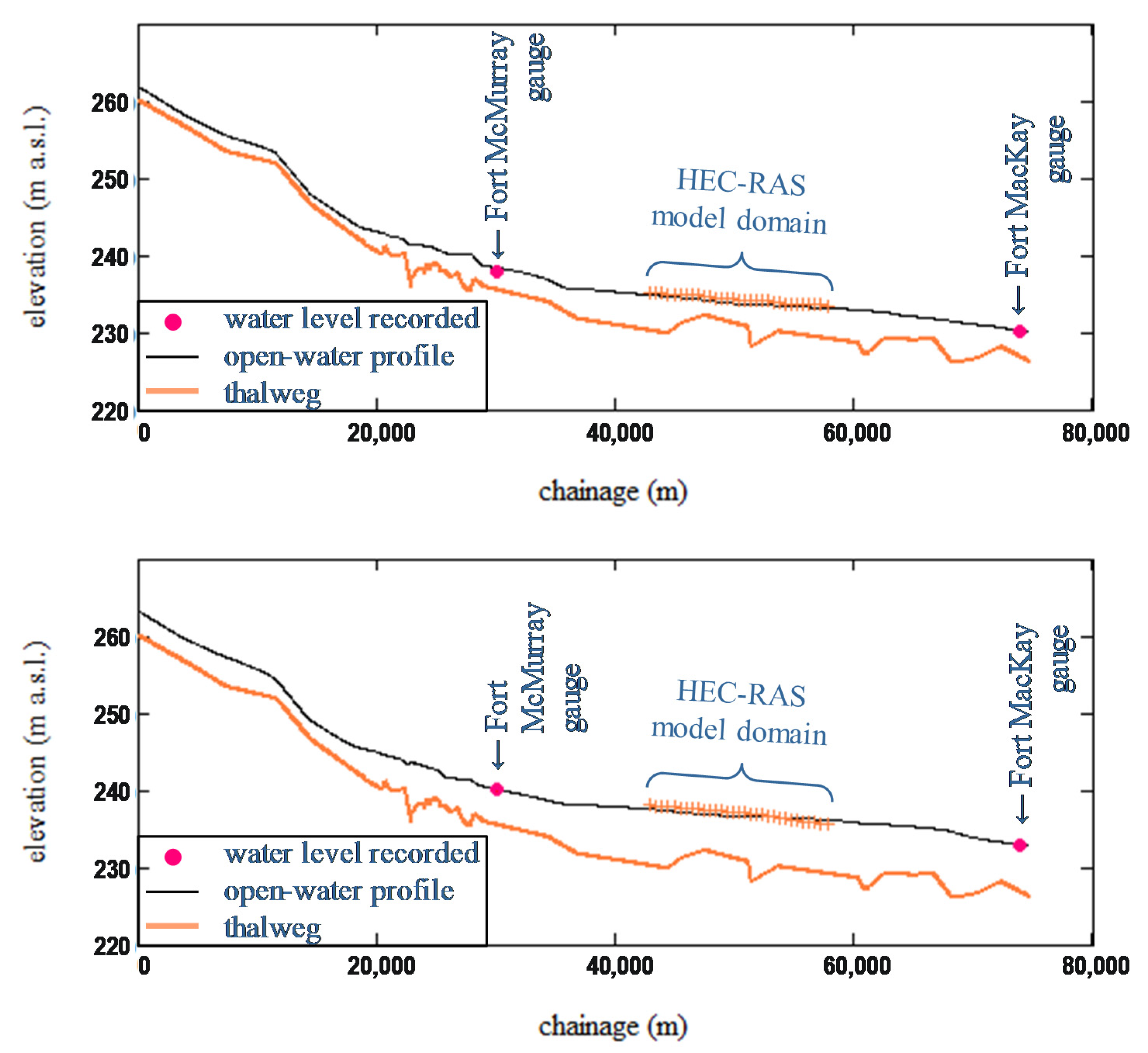
Water level gauges are not present within the 15 km modelling domain. There is an active gauge (records from 1957 to present) at the Water Survey of Canada (WSC) station approximately 13 km upstream of the modelling domain at Fort McMurray (gauge 07DA001–Athabasca River below Fort McMurray) and a discontinued gauge (recordings only from 1959 to 1966) approximately 16 km downstream of the modelling domain at Fort MacKay (gauge 07DA003–Athabasca River near Fort MacKay). The average flow at the gauge at Fort McMurray is about 600 m3/s. This flow was used to calibrate the WASP simulations of tracer mixing from a hypothetical outfall from the right bank at the upstream boundary of the model domain. A flow of 2800 m3/s was used for validation and to simulate flow from the Athabasca River into Shipyard Lake.
The hydraulic model HEC-RAS [
20], developed by the U.S Army Corps of Engineers, was used to generate the segmentation for the WASP water quality model. The water level elevations of the HEC-RAS model at flows 600 and 2800 m
3/s, which formed the geometrical basis for the WASP segmentation, were verified with flow simulations using the hydraulic model ONE-D, a hydrodynamic model that uses a finite difference implicit scheme for the solution ([
21,
22] both referenced in [
23]). Both mass and momentum of sub-critical fluid motion are conserved for open-channel flow. The model is robust and well-tested with many consultancy applications (e.g., [
24,
25]). Bathymetry data were obtained from Alberta Environment and Parks (AEP) [
26].
Figure 7 shows how the water level profiles modelled in ONE-D match with the water level elevations recorded at the gauges at Fort McMurray and Fort MacKay for an average flow of 600 m
3/s and a higher flow of 2800 m
3/s. The water level elevations modelled with HEC-RAS for the same steady-state flow coincide well with the ONE-D water level profile.
4. Water-Quality Modelling Setup
The Water Quality Analysis Simulation Program (WASP 8.32) was used to model the water quality of the river-lake system. WASP is a general dynamic model that applies a segmentation network to solve the conservation of momentum, energy, and mass equations and simulate contaminant and sediment transport. WASP was initially developed in the 1980s and has undergone many upgrades since then. WASP is a widely used model, especially in North America, for addressing various environmental and water quality concerns. The WASP segmentation can be structured in 1D for streams, or 2D for rivers with branching channels or 3D for lakes.
The WASP stream transport module, TOXI, is able to calculate the flow of water, sediment and dissolved constituents through branched and ponded segments and is coupled with flow routing for free flow streams, ponded segments, and backwater reaches. The kinematic wave was used for the 1D flow routing, which is based on solutions of one-dimensional continuity equations and a simplified form of the momentum equation that considers effects of gravity and friction, and calculates variations in velocities, widths and depths throughout the network. Flow through the ponded segments is calculated based on a sharp-crested weir equation, which calculates outflow based on water elevation above the weir crest, using kinematic wave flow for a river and ponded weir overflow for a lake. For the current study, boundary and initial conditions were defined based on water quality data of the closest station to the study area by spatial linear interpolation.
Input data for the model includes channel geometry, flow routing, boundary conditions, environmental time functions, loads and initial conditions for segments. Geometry for the WASP segments (average depths, widths and slopes) was extracted from the fifty-eight HEC-RAS cross-sections, which were spaced at a distance of 493 m apart. Segments are a series of discretized components used to estimate the model state variables at every time step. The sediment transport model is an independent set of routines with associated parameters for the model.
The domain was modelled with a network of river segments, a secondary channel and a side lake. Water quality modelling of such a complex system requires special consideration of the varying hydrodynamics within the system. The primary segments of the system are 493 m long; as mentioned before, right stream segments accommodate 20% of the width of cross-sections produced by HEC-RAS for the 600 m3/s scenario and 10% of the width for the 2800 m3/s flow scenario.
Bathymetric information for Shipyard Lake was obtained from a bathymetry survey carried out by Golder [
17]. The lake was divided into two segments:
As mentioned above, the mixing length for the stream is long, and the geographical complexity of the study area cannot be represented with a 1D modelling approach alone. On the other hand, a 2D approach would require higher data computational resources for such a long stream. Quasi-2D models can be a reasonable alternative by using the simplicity of a 1D solution but still capturing 2D discretisation of the substance transport. The approach is purely a balance of water and mass between each adjoining segments. This includes the exchange of water and mass between each adjacent-lying, left and right stream segments. The exchange is a small percentage of the water flowing into each of those segments from their upstream segments. The exchange alternates from right-to-left and left-to-right stream segments along the model domain. The flow exchange was calibrated in such a way that the constituents within the two streams mixed together more and more as we moved further downstream along the domain. The flow transfers between adjacent segments were calibrated so that the concentrations matched the observed dispersion pattern calculated with the Athabasca River Model (ARM). Concentration gradients were generally higher between the left and right stream segments at the upstream boundary leading to more rapid mixing in this area; as we move further downstream, the mixing between the adjacent segments of each stream led to a decrease in their concentration gradients and a decrease in the mixing rate.
In this study, results from one model, ARM, were used to calibrate the mixing simulated with WASP. However, field data sampled not only longitudinally along the flow direction of the river, but also transversely across the river can be used to calibrate the model, an example of which is provided in a follow-up study to simulate the transport of vanadium [
27].
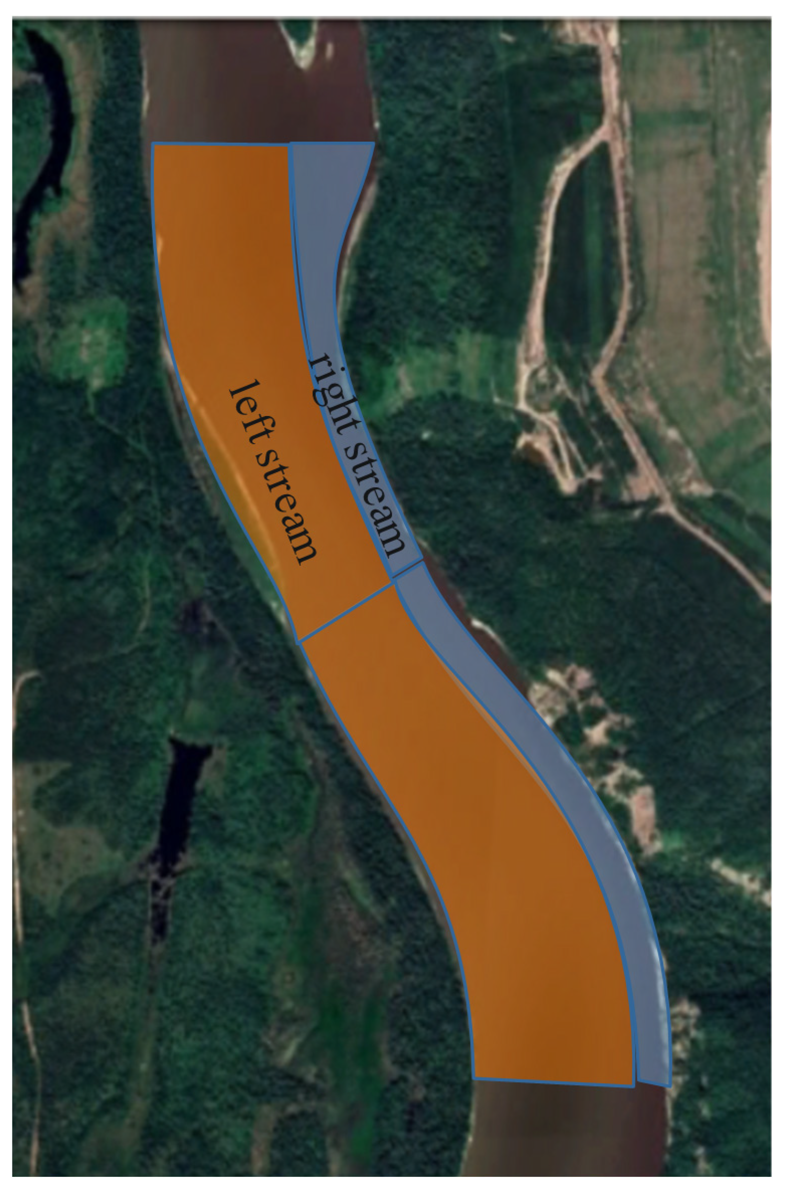
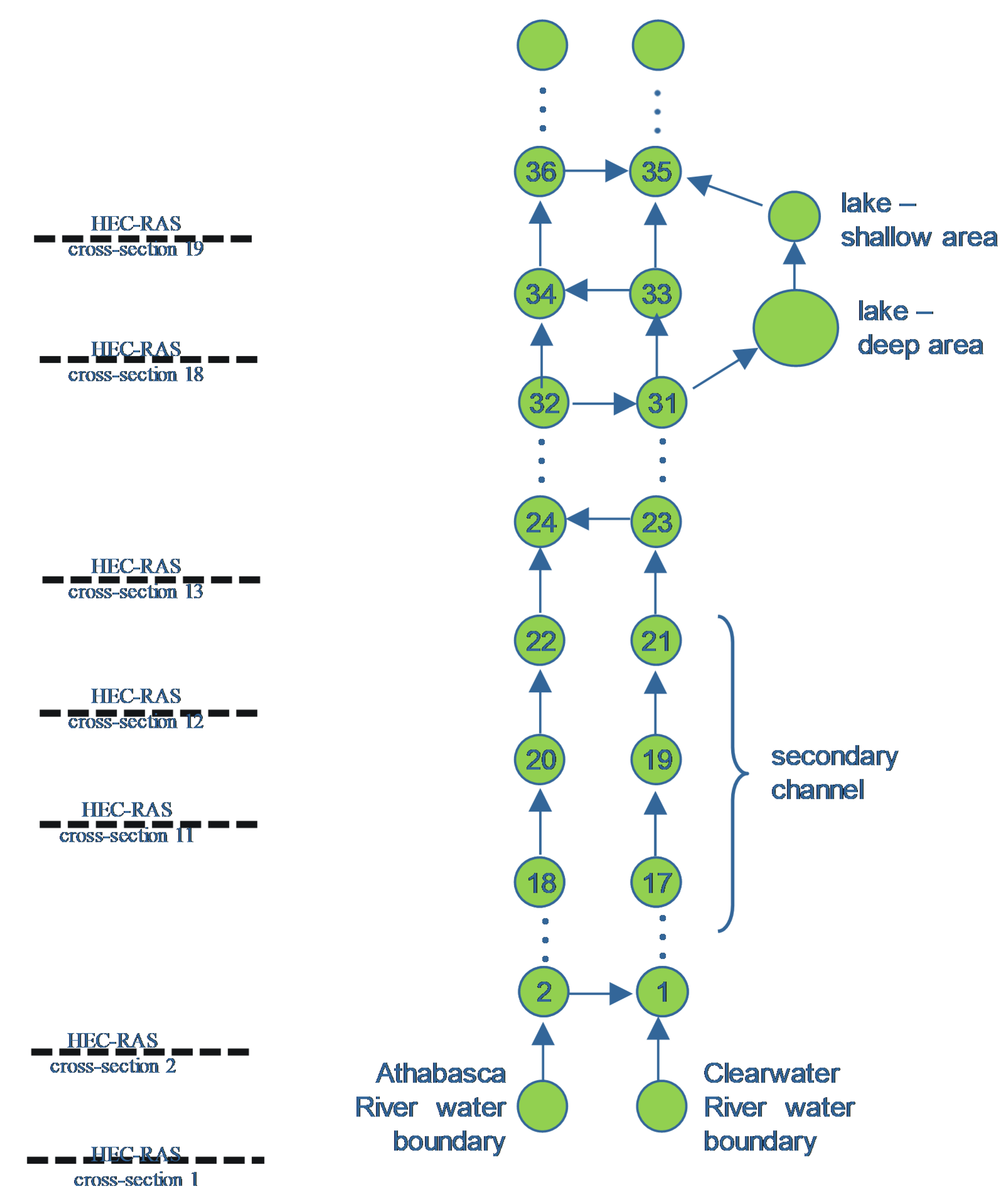
The stretches between every two cross-sections of the HEC-RAS model were divided into two stream tubes. The flow from the Clearwater River controlled the segment on the right side (right stream), and the main Athabasca River system controlled the segments on the left side (left stream), as shown in
Figure 8. Flow for the secondary channel was supplied through the right side stream. It was estimated that 2% of flow into Shipyard Lake was required to maintain water volume continuity. The flow through Shipyard Lake was anticipated to flow back into the right side stream just downstream of the lake. A schematic of the segmentation is shown in
Figure 9.
In order to characterize erosion and sedimentation, benthic segments were added under each surface water segment. Solids can be separated into clay, silt and sand, which can refine simulation results of solids. The user has four choices for simulating solids in WASP: solid flow fields, descriptive, the mechanistic Van Rijn equation, and the mechanistic Robert equation. Currently, WASP has two kinetic modules for modelling sediment transport. For the current study, the advanced toxicant module was used because it is considered to be the best module to simulate oil-sands associated substances.
5. WASP Mixing Calibration (Q = 600 m3/s)
Calibration of the mixing of the WASP model was done using simulation results from the Athabasca River Model (ARM) [
16,
17]. ARM is a vertically averaged, two-dimensional mixing model used to predict substance concentrations varying across the width and length of the lower Athabasca River for various flow conditions. The model’s calculations are analytical/explicit in nature, so there is no discretization other than differentiating between different reaches with different mixing and hydraulic parameters. ARM applies analytical solutions for river dispersion equations under steady-state conditions. Mid-field mixing is represented by dispersion equations described by Fischer et al. [
28]. The same representation is used for passive ambient mixing in the Cornel Mixing Zone Expert System (CORMIX) [
29] except that, for ARM, transverse mixing coefficients have been calibrated based on a tracer-dye study completed in 2003 [
30,
31] and validated using a range of data sources [
32]. The calibration of ARM is described in [
30,
31].
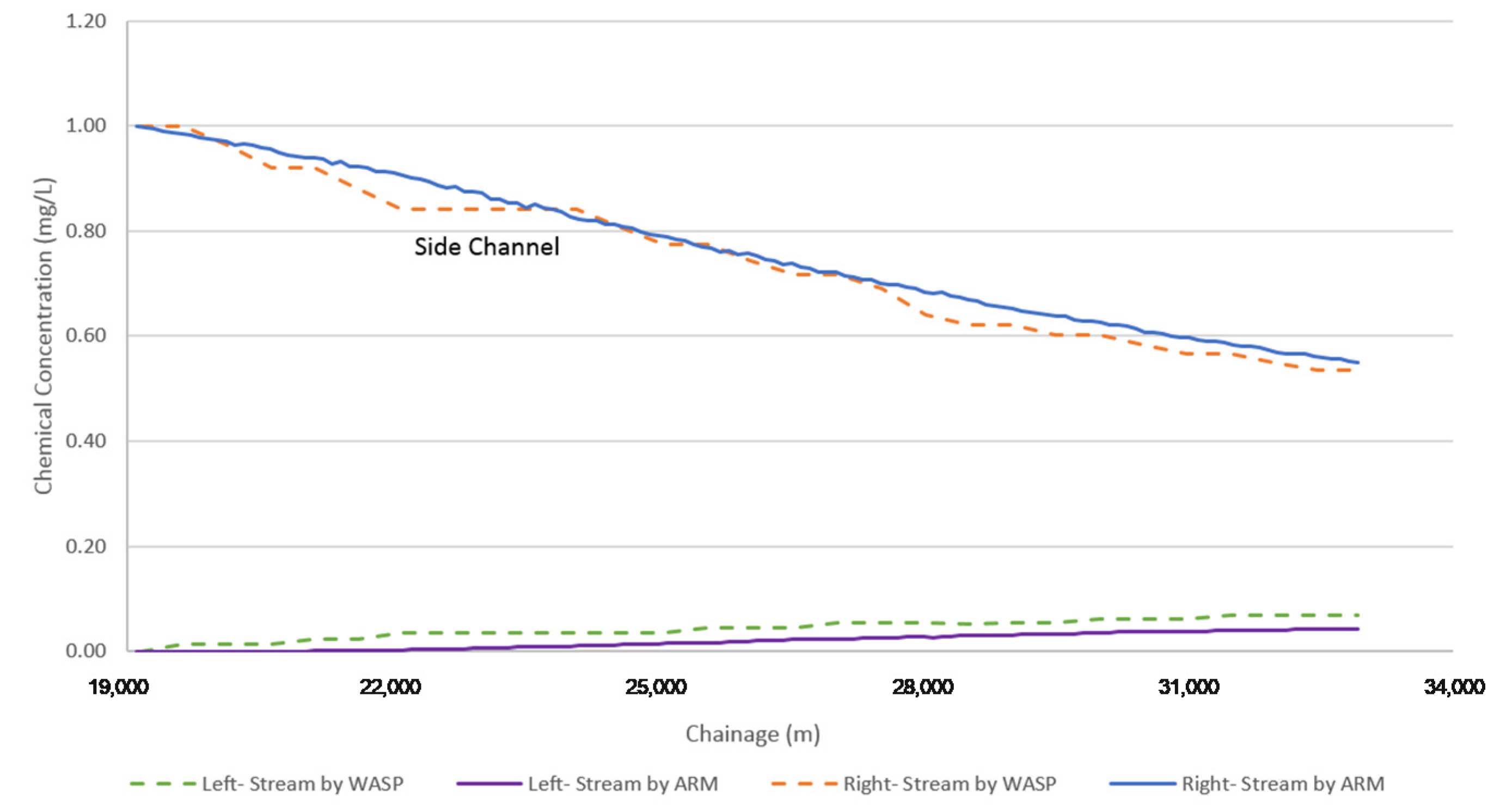
A hypothetical conservative tracer was chosen to calibrate the mixing path of the WASP model to the ARM predictions. A load of 5670 kg/day, which led to the chemical concentration of 1 mg/l in the most-upstream segment (Segment 1) was added. The flow system included two upstream boundary conditions: the Athabasca River water for the left stream boundary and the Clearwater River water for the right stream boundary.
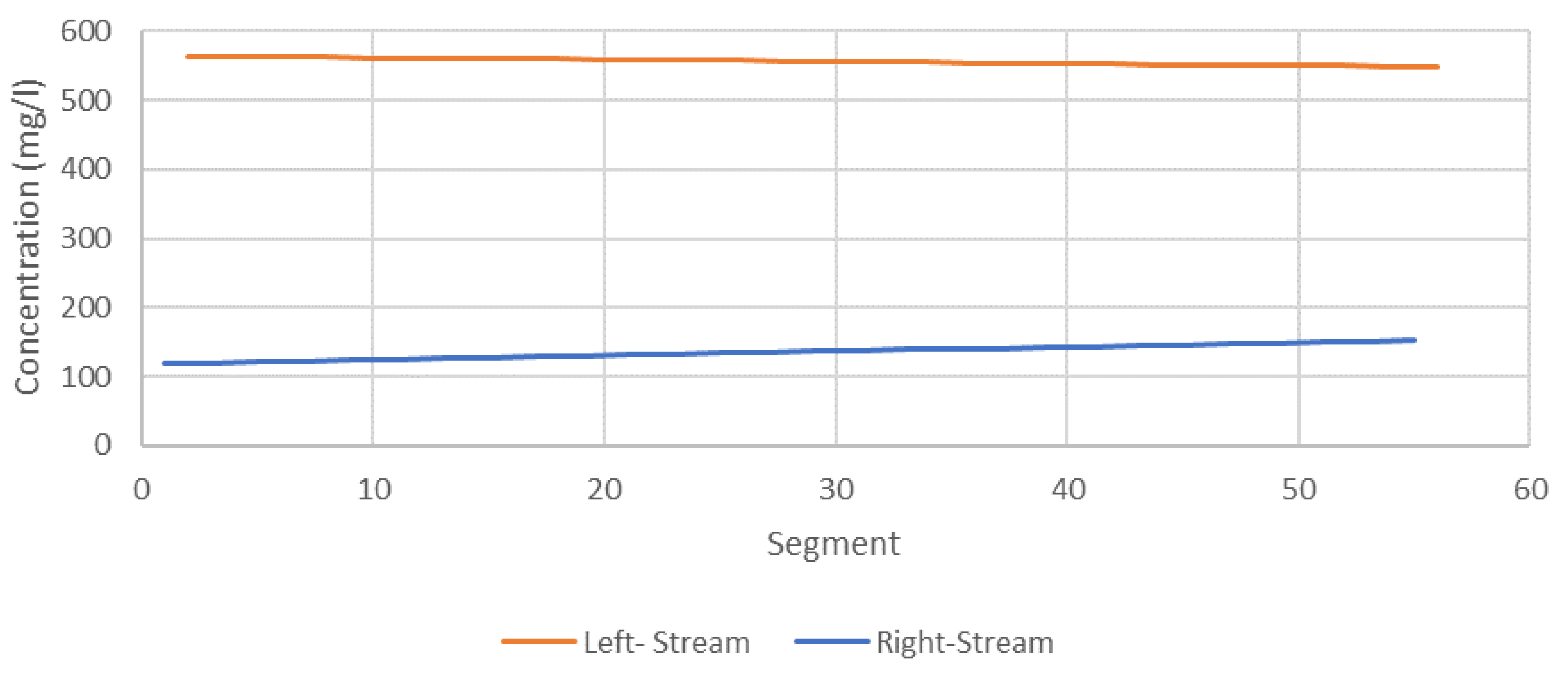
As expected, the conservative tracer was transported to the left stream when a flow was designated between them. Segments divided by islands (segment combinations 16–17, 18–19 and 20–21) had no flow between them. WASP simulated the concentrations of the tracer in each segment. These values were compared with values predicted by the ARM model and shown in
Figure 10.
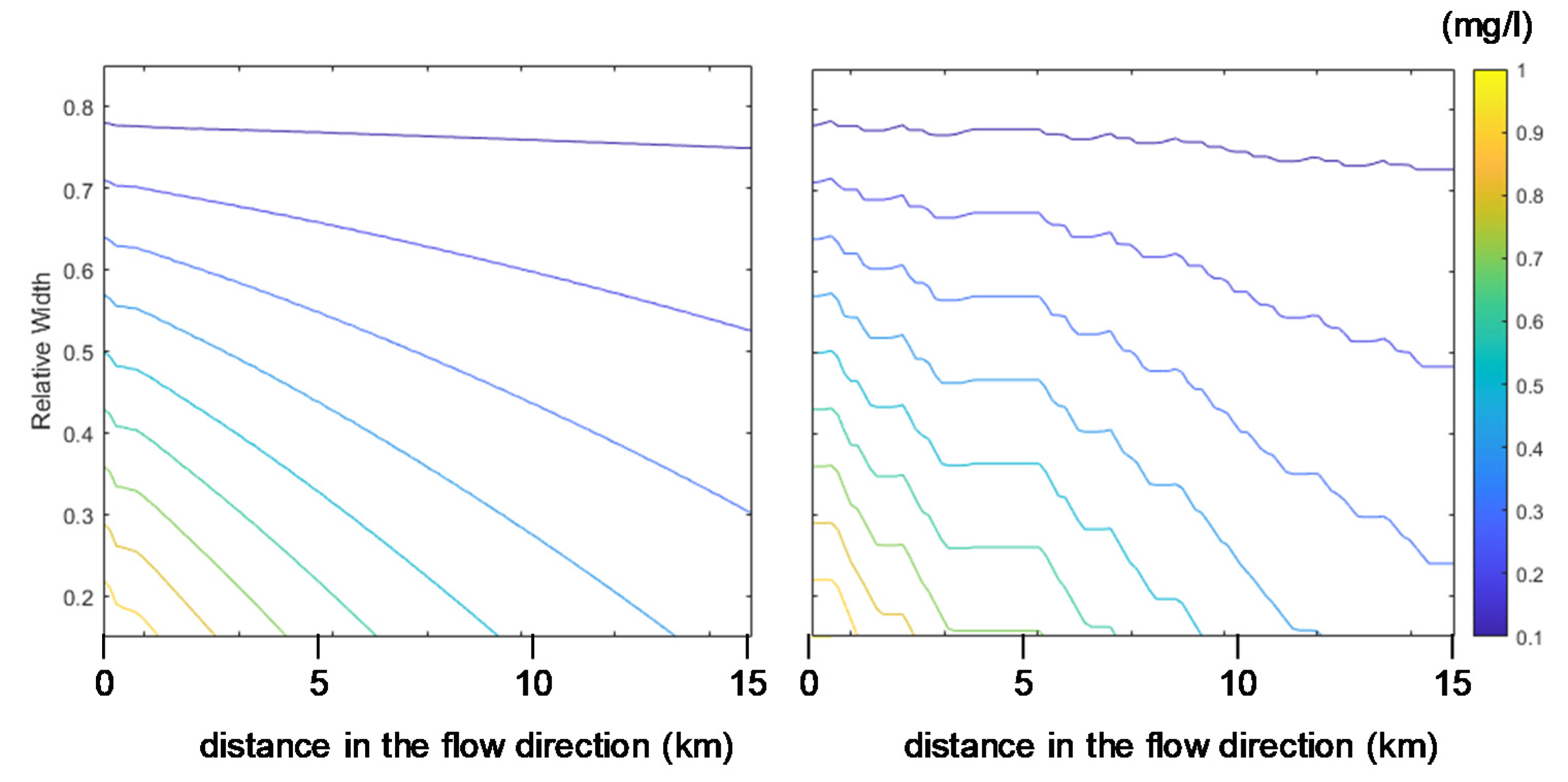
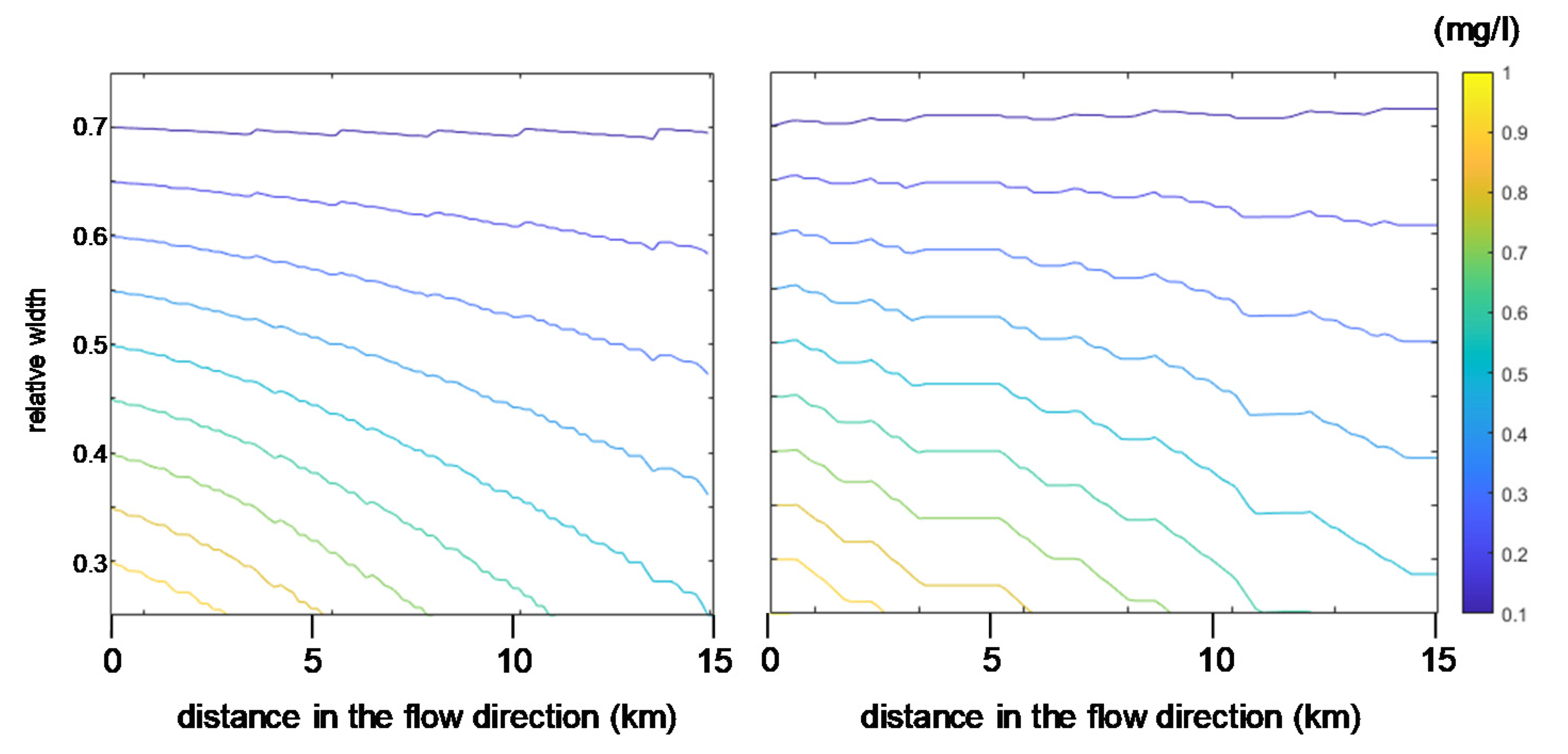
Good agreement for both left and right streams was observed. As can be seen, both models predicted the same trend for both streams: a reduction in chemical concentrations in the right stream and an increase in chemical concentrations in the left stream. Contour plots of the tracer concentrations modelled in WASP and ARM are shown in
Figure 11.
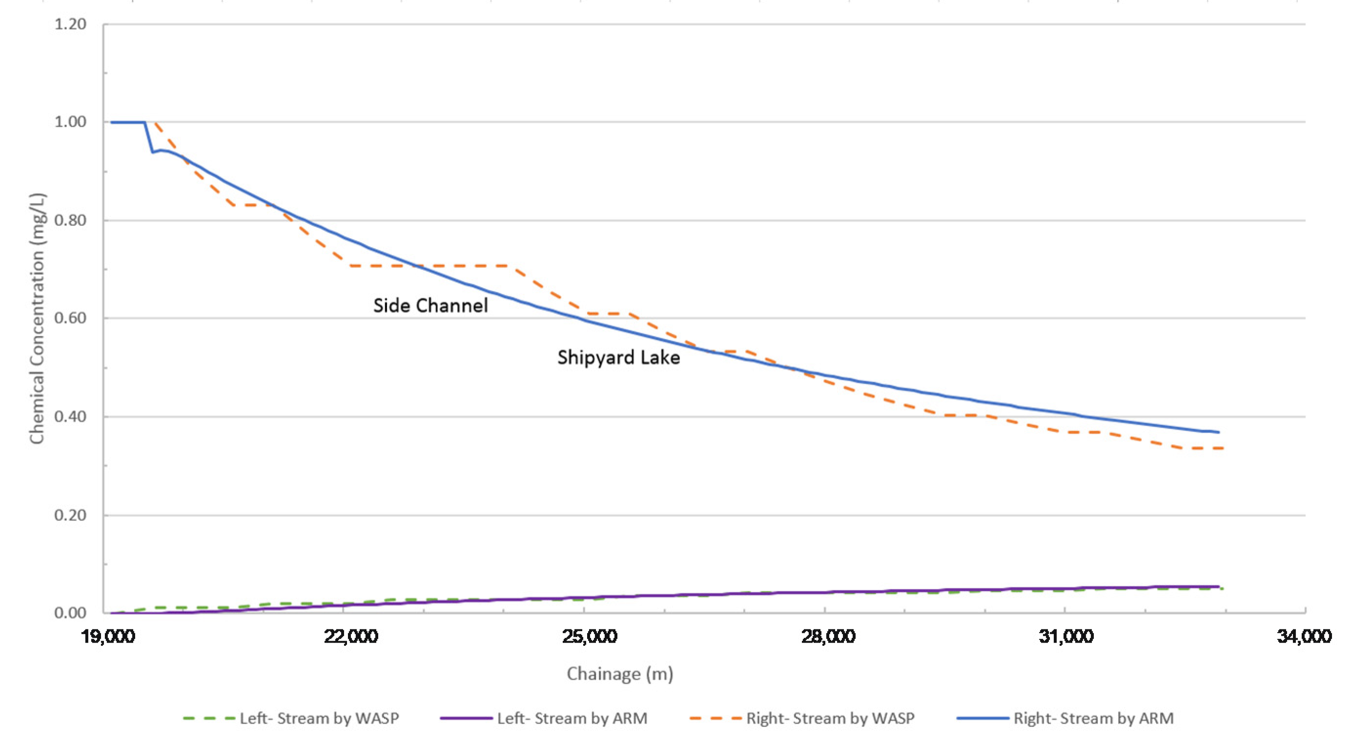
6. WASP Mixing Validation (Q = 2800 m3/s)
A simulation with a higher flow of 2800 m
3/s was carried out for which both Shipyard Lake and the secondary channel became flooded. The results of the two models for the two streams are shown in
Figure 12. Again, mixing is evident since the tracer concentrations are increasing in the right stream and decreasing in the left stream, both in the flow direction. Mixing is more rapid for the 2800 m
3/s scenario since the tracer concentrations drop to 40% of the original concentration at the end of the 15 km stretch, whereas the concentrations only drop to 55% in the 600 m
3/s scenario (
Figure 10). Contours of the tracer concentrations simulated in ARM and WASP are provided for the 2800 m
3/s flow case in
Figure 13. The same trend for the mixing was observed for both flow rates studied herein. For the higher flow rate, faster mixing was observed, which can be explained by higher turbulence and more chaotic eddies which follow observations by Dimotakis [
33] and Sreenivasan [
34].
7. Sediment Transport Modelling
Suspended solids and benthic sediments are key components of the water quality of rivers and lakes. When the flow velocity decreases, as is the case when, for example, a river flows into a lake or reservoir, suspended sediments will settle out. Key constituents in oil sands process water, such as selenium and polycyclic aromatic hydrocarbons, tend to sorb to fine sediments. For the current study, separate size classes were represented using the descriptive solids transport option in WASP. For the descriptive solids transport, constant settling and resuspension velocities were defined for each segment. Settling velocity of silt and clay were calculated from Stokes Law, and the settling velocity of sand was estimated based on the equation from Ferguson and Church [
35].
Size classes for suspended solids were estimated based on suspended sediment samples collected from the Lower Athabasca River using continuous flow centrifugation in 2012 and 2013 as part of the Joint Oil Sands Monitoring Program [
1].
Measured TSS data were fitted versus the flow rate for the sediment sampling stations. Power functions were used to fit the data yielding acceptable r
2 values (r
2 > 0.6) for all correlations. This provided equations to estimate TSS based on the given flow rates. For the sediment transport simulation, we used the flow scenario of 2800 m
3/s because at that flow, both the secondary channel and Shipyard Lake are flooded by Athabasca River water. A flow of 2800 m
3/s corresponds to a flow of 250 m
3/s for the Clearwater River (from
Figure 5), and a flow of 2550 m
3/s along the upper Athabasca River reach, which represents a flow ratio of approximately 10–90%, respectively. Although the model domain is situated downstream of the Athabasca/Clearwater river confluence, for the purpose of showing proof-of-concept in this study, the 10/90 percentage ratio was maintained for the right/left streams.
After obtaining TSS values for the flow scenario for the water quality stations, an interpolation was done to obtain initial sediment concentrations for each segment along the study area (see
Figure 14). For segments on the right stream (segments with odd numbers), linear interpolation between Clearwater River at Draper and Athabasca/Firebag confluence was carried out. For left stream segments (segments with even numbers), values were interpolated between the station upstream of the Athabasca/Clearwater confluence and Athabasca/Firebag confluence. After obtaining TSS amounts for each segment, the average ratio of long-term means was used to estimate the concentration of silt, clay and sand in each segment. Initial concentrations for benthic segments were estimated from available bed sediment data for the Lower Athabasca River collected as part of the Regional Aquatics Monitoring Program [
36].
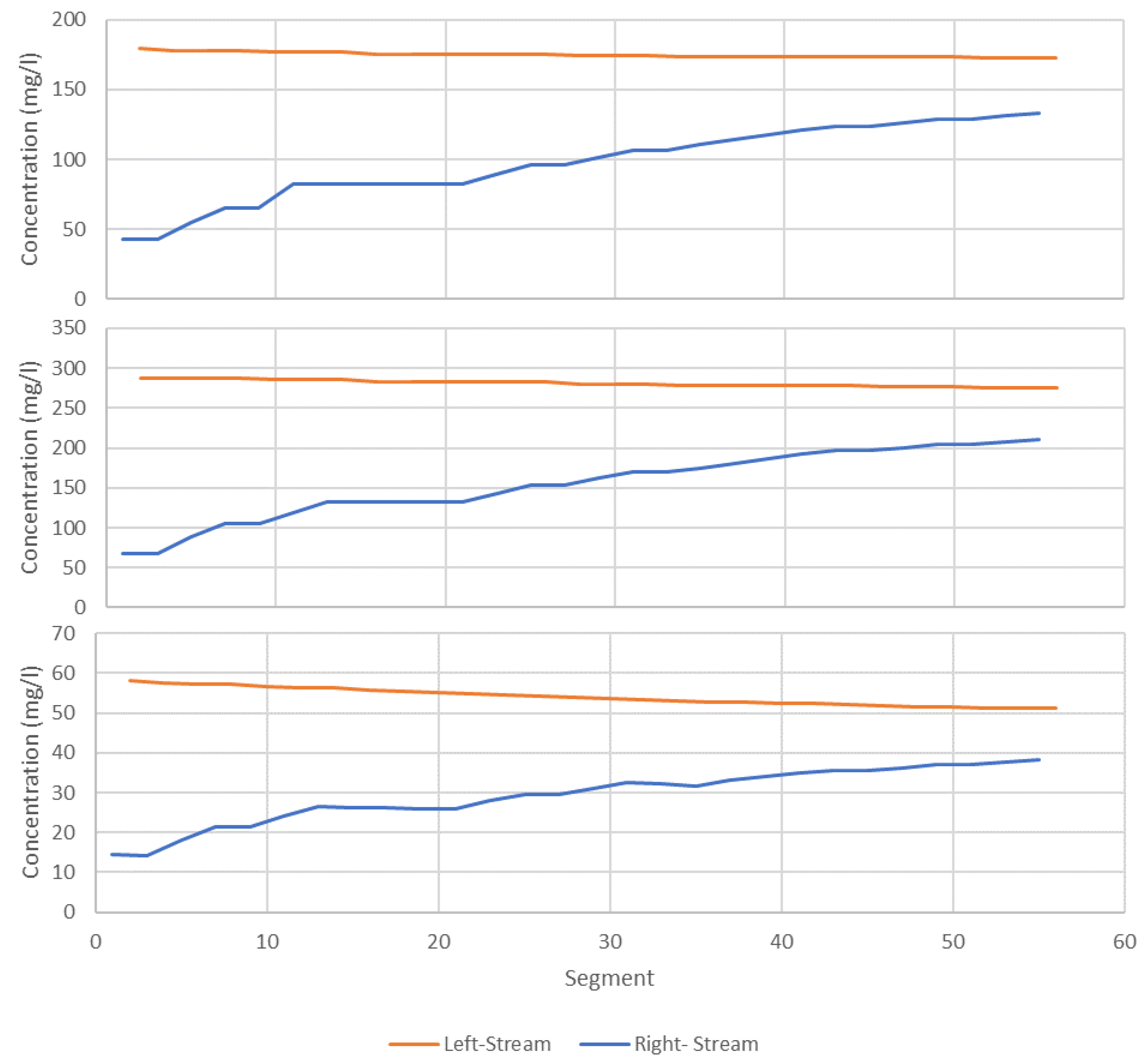
The model was run until it reached an equilibrium state, after which no significant changes in the sediment concentrations in the surface water segments were observed. It was assumed that an equilibrium state has been reached when there was no significant change in sediment concentration in the water body for more than a simulation time of 24 h. For the current study, clay, silt and sand were modelled, and the results of these for both the left and right streams of the Athabasca River are shown in
Figure 15.
The mechanics of solid transport in WASP are based on advection, and suspended sediments are only transported transversely when there is a flow routed between segments of the right and left streams. It is evident that the left stream segments have higher sediment concentrations than the right stream segments. In addition, sediment concentrations tend to drop in the left stream and increase in the right stream, both with flow direction, which is attributed to the transverse mixing, as is the case for the tracer simulations.
For all segments, including left and right streams, it was observed that, for the water columns, the amount of sediments decreases in order from silt, to clay and then sand. Due to the higher settling velocity for sand, it can be expected that there would be more sand deposits in the river compared to silt and clay. Sand is typically transported as a bedload or during higher velocity flows due to its roughness and higher density [
37,
38,
39]. Due to its low settling velocity, clay is the dominant sediment texture in the water column.
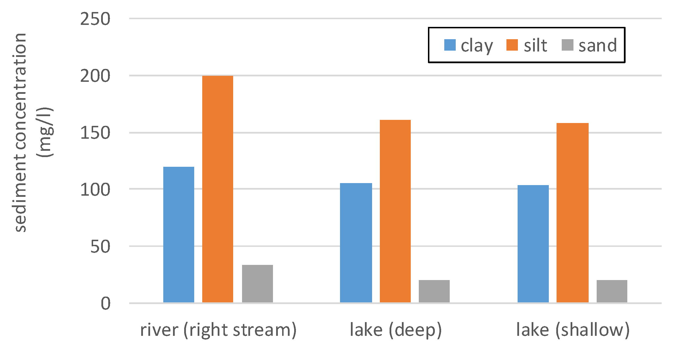
At Shipyard Lake, a considerable deposition of sediment in the lake was simulated compared to the sediment in the right stream of the Athabasca River (see
Figure 16). The flow through the lake is in the direction of: right stream → deep part → shallow part → right stream (further downstream). The higher sedimentation in the lake is due to the drop in flow velocity of the water entering the lake. Much of the sediment of all three textures is deposited in the deeper part of the lake with some additional deposition in the shallow lake area. The amount of solids increases in the surface benthic segments because settling dominates over resuspension in the lake.
The simulations with WASP were very fast, taking only about 30 s for the model to reach steady state. This is much faster than a two-dimensional approach that was carried out in which a “relatively coarser grid was used for all of the main chemical constituent runs due to their higher computational requirements” [
40]. Our approach presented here would be an alternative to creating a second grid.
8. Summary and Conclusions
A novel methodology was proposed to simulate transverse mixing along a long stream of a river network with a secondary channel and side lake. A steady-state water quality model based on two flow scenarios (600 and 2800 m3/s) was developed to study transverse mixing and sediment deposition in the modelling domain.
The first objective of this study was to model transverse mixing in the river-lake system. Good agreement with the previously developed ARM model was observed. It was established that a quasi-2D approach is a reasonable and accurate means of modelling transverse mixing of the system with a minimal processing time compared to more complex 2D models. The approach is also well suited for scaling up to a larger river network in future work by extending the modelling domain from Fort McMurray to the Athabasca Delta.
The second objective was to quantify deposition of sediments along the system. As expected, much of the sediment load deposits are found within the secondary channel and the side lake, with less deposition in the main channel. It was observed that coarser materials tend to deposit in the deep part of the lake, where the Athabasca River water first enters the lake. Due to the longer settling time for finer sediments, they were the main sediments suspended in the main stem.
The last objective was to emphasize the importance of drawing on the output from additional models to complement the water-quality modelling exercise. To support the water-quality modelling with WASP, the hydrodynamics of the water-quality modelling domain was analyzed using HEC-RAS and ONE-D. The ONE-D model has an extended domain that incorporates recordings from gauge stations. The calibrated and validated ARM model was also useful to calibrate the transverse mixing within the WASP model. Should we scale up to extend the modelling stretch from Fort McMurray to the Athabasca Delta, additional models, in particular a hydrological model of the Athabasca River basin, should also be included. This will be essential to predict the state of the river’s water quality under a changing climate scenario in the future. The impacts of an ice cover on the river’s water quality should also be considered in future research.
Author Contributions
Conceptualization, T.R. and K.-E.L.; methodology, K.-E.L.; model setup, E.A. and P.S.; calibration, P.S. and K.-E.L., validation, P.S.; formal analysis, P.S. and K.-E.L.; investigation, P.S., T.R. and K.-E.L.; resources, T.R. and K.-E.L.; data curation, T.R. and K.-E.L.; writing—original draft preparation, P.S. and K.-E.L.; writing—review and editing, T.R. and K.-E.L.; supervision, T.R. and K.-E.L.; project administration, T.R. and K.-E.L.; funding acquisition, T.R. and K.-E.L. All authors have read and agreed to the published version of the manuscript.
Funding
This research was funded by Alberta Environment and Parks and the Integrated Modelling Program for Canada (IMPC) under the University of Saskatchewan’s Global Water Futures (GWF) program.
Institutional Review Board Statement
Not applicable.
Informed Consent Statement
Not applicable.
Conflicts of Interest
The authors declare no conflict of interest. The funders had no role in the design of the study; in the collection, analyses, or interpretation of data; in the writing of the manuscript, or in the decision to publish the results.
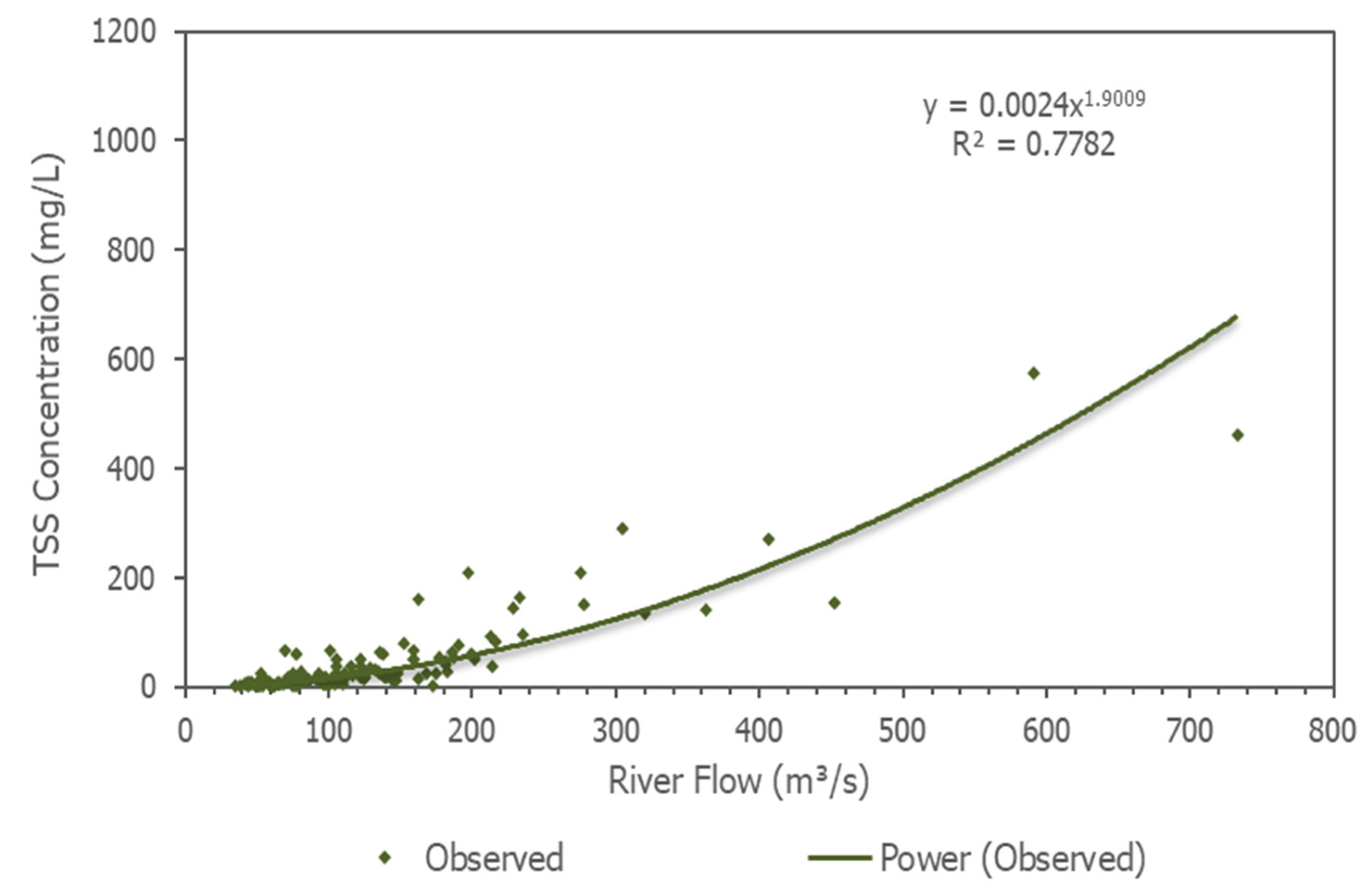
Appendix A
Figure A1.
Total suspended sediment vs. flow for Athabasca River upstream of Fort McMurray.
Figure A1.
Total suspended sediment vs. flow for Athabasca River upstream of Fort McMurray.
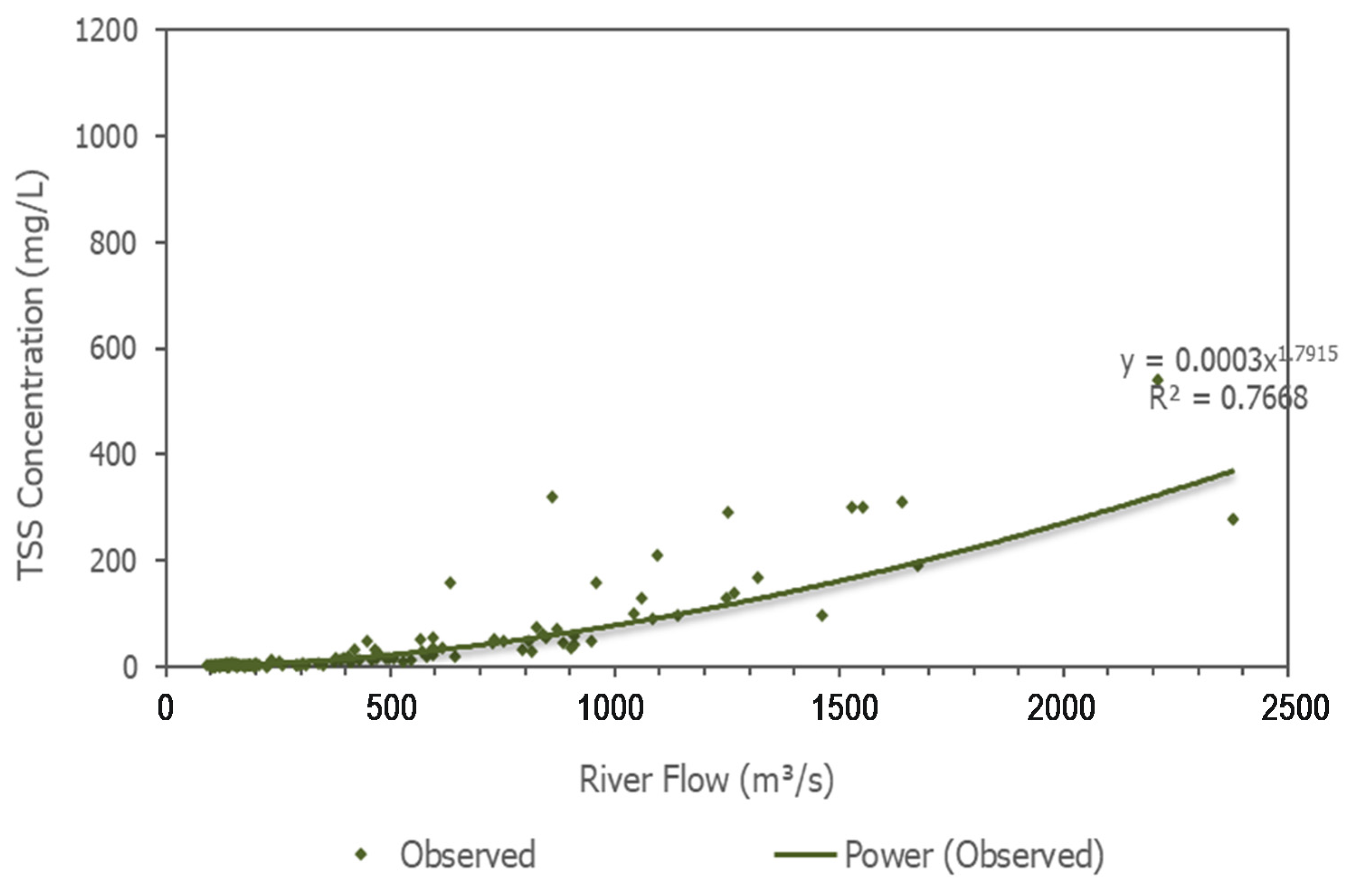
Figure A2.
Total suspended sediment vs. flow for Clearwater River.
Figure A2.
Total suspended sediment vs. flow for Clearwater River.
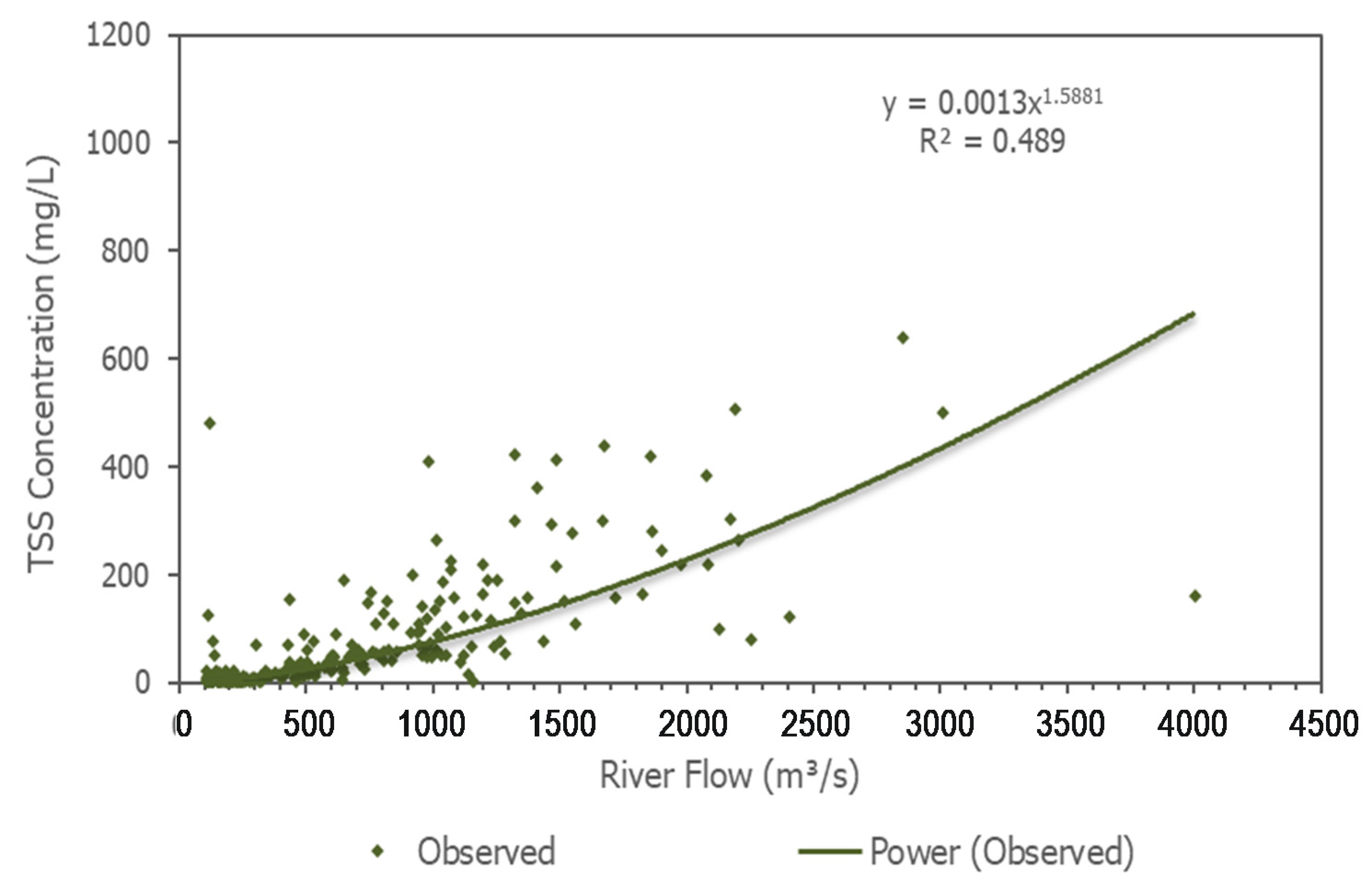
Figure A3.
Total suspended sediment vs. flow for Athabasca River upstream of Firebag River.
Figure A3.
Total suspended sediment vs. flow for Athabasca River upstream of Firebag River.
Figure A4.
Total suspended sediment vs. flow for Athabasca River at Old Fort.
Figure A4.
Total suspended sediment vs. flow for Athabasca River at Old Fort.
References
- ECCC Canada-Alberta Joint Oil Sands Monitoring Program-Suspended Sediment Monitoring Disclaimer and Notes, Environment and Climate Change Canada. 2021. Available online: https://donnees.ec.gc.ca/data/substances/monitor/sediment-oil-sands-region/sediment-quality-mainstem-and-tributaries-oil-sands-region/?lang=en (accessed on 1 November 2021).
- Gupta, A.; Farjad, B.; Wang, G.; Eum, H.; Dubé, M. Integrated Environmental Modelling Framework for Cumulative Effects Assessment; University of Calgary Press: Calgary, AB, Canada, 2021. [Google Scholar]
- EPA. Water Quality Analysis Simulation Program (WASP), Environmental Protection Agency. Available online: https://www.epa.gov/ceam/water-quality-analysis-simulation-program-wasp (accessed on 1 November 2021).
- Wool, T.; Ambrose, R.B., Jr.; Martin, J.L.; Comer, A. WASP 8: The Next Generation in the 50-year Evolution of USEPA’s Water Quality Model. Water 2020, 12, 1398. [Google Scholar] [CrossRef] [PubMed]
- Lindenschmidt, K.-E.; Pech, I.; Baborowski, M. Environmental risk of dissolved oxygen depletion of diverted flood waters in river polder systems-a quasi-2D flood modelling approach. Sci. Total Environ. 2009, 407, 1598–1612. [Google Scholar] [CrossRef] [PubMed] [Green Version]
- Lindenschmidt, K.-E. Quasi-2D approach in modelling the transport of contaminated sediments in floodplains during river flooding-model coupling and uncertainty analysis. Environ. Eng. Sci. 2008, 25, 333–352. [Google Scholar] [CrossRef] [Green Version]
- Lindenschmidt, K.-E.; Huang, S.; Baborowski, M. A quasi-2D flood modelling approach to simulate substance transport in polder systems for environmental flood risk assessment. Sci. Total Environ. 2008, 397, 86–102. [Google Scholar] [CrossRef] [PubMed]
- Sehnert, C.; Lindenschmidt, K.-E. The effect of upstream river hydrograph characteristics on zinc deposition, dissolved oxygen depletion and phytoplankton growth in a flood detention basin system. Quat. Int. 2009, 208, 158–168. [Google Scholar] [CrossRef]
- Huang, S.; Vorogushyn, S.; Lindenschmidt, K.-E. Quasi 2D hydrodynamic modelling of the flooded hinterland due to dyke breaching on the Elbe River. Adv. Geosci. 2007, 11, 21–29. [Google Scholar] [CrossRef] [Green Version]
- Huang, S.; Rauberg, J.; Apel, H.; Disse, M.; Lindenschmidt, K.-E. The effectiveness of polder systems on peak discharge capping of floods along the middle reaches of the Elbe River in Germany. Hydrol. Earth Syst. Sci. 2007, 11, 1391–1401. [Google Scholar] [CrossRef] [Green Version]
- Sehnert, C.; Huang, S.; Lindenschmidt, K.-E. Quantifying structural uncertainty due to discretisation resolution and dimensionality in a hydrodynamic polder model. J. Hydroinformatics 2009, 11, 19–30. [Google Scholar] [CrossRef]
- Cunge, J.A. Two-dimensional modeling of floodplains. In Unsteady Flow in Open Channels; Mahood, K., Yevjevich, V., Eds.; Water Resources Publications: Fort Collins, CO, USA, 1975; Volume 2, pp. 705–762. [Google Scholar]
- Aureli, A.; Maranzoni, A.; Mignosa, P.; Ziveri, C. Flood hazard mapping by means of fully-2-D and quasi-2-D numerical modeling: A case study. In Floods, From Defence to Management; van Alphen, J., van Beek, E., Taal, M., Eds.; 3rd International Symposium on Flood Defence: Nijmegen, The Netherlands; Taylor and Francis/Balkema: Blain, France, 2006; pp. 373–382. ISBN 0415391199. [Google Scholar]
- Asselman, N.E.M.; Van Wijngaarden, M. Development and application of a 1-D floodplain sedimentation model for the River Rhine in the Netherlands. J. Hydrol. 2002, 268, 127–142. [Google Scholar] [CrossRef]
- OSEM. Oil Sands Environmental Monitoring. 2021. Available online: https://www.environment.alberta.ca/apps/OSEM/ (accessed on 31 July 2021).
- Golder. Reach-Specific Water Quality Objectives for the Lower Athabasca River; Golder Associates Ltd. for Cumulative Environmental Management Association: Fort McMurray, AB, Canada, 2007. [Google Scholar]
- Golder. Aquatic Baseline Report for the Athabasca, Steepbank and Muskeg Rivers in the Vicinity of the Steepbank and Aurora Mines (Appendices); Golder Associates Ltd. for Suncor Inc.: Calgary, Alberta, Canada, 1996. [Google Scholar]
- Klohn-Crippon. Hydrology Baseline for Project Millenium; Report PA 289.03 submitted to Suncor Energy Inc. by Klohn-Crippon, Publisher: Vancouver, BC, Canada, 13 April 1998; Available online: chttps://era.library.ualberta.ca/items/2f3407d5-193a-4a9e-b2cb-633ffd7c8a3f/view/cc88c7c8-781a-44a5-934c-ecd4aaf5d0b4/2A-2_-_Hydrology_Baseline_for_Project_Millennium.pdf (accessed on 1 November 2021).
- Newman, K.T. An Integrated Analysis of Sediment Geochemistry and Flood History of Floodplain Lakes in the Athabasca Region. Ph.D. Thesis, University of Saskatchewan, Saskatoon, SK, Canada, 2019. Available online: https://harvest.usask.ca/handle/10388/12436 (accessed on 1 November 2021).
- USACE. HEC-RAS River Analysis System–User’s Manual Version 6.0. US Army Corps of Engineers Hydrologic Engineering Center. 2021. Available online: https://www.hec.usace.army.mil/software/hec-ras/documentation/HEC-RAS_6.0_Users_Manual.pdf (accessed on 31 July 2021).
- Dailey, J.E.; Harleman, D.R.F. Numerical Model for the Prediction of Transient Water Quality in Estuary Networks; Report # 158, RT72-72; Hydrodynamics Laboratory, Massachusetts Institute of Technology: Cambridge, MA, USA, 1972. [Google Scholar]
- Morse, B. St-Lawrence River Water-Levels Study: Application of the ONE-D Hydrodynamic Model; Transport Canada, Waterways Development Div., Canadian Coast Guard: Ottawa, ON, Canada, 1990. [Google Scholar]
- Matte, P.; Secretan, Y.; Morin, J. Hydrodynamic modeling of the St. Lawrence fluvial estuary, 1: Model setup, calibration and validation. J. Waterw. Port Coast. Ocean Eng. 2017, 143, 04017010. [Google Scholar] [CrossRef]
- Sydor, M.; DeBoer, A.; Cheng, T. Developing a Mathematical Flow Simulation Model for the Peace-Athabasca Delta; Environment Canada and Alberta Environment: Edmonton, AB, Canada, 1979; Available online: http://www.worldcat.org/oclc/70366515 (accessed on 1 November 2021).
- Sydor, M.; Kassem, A.; Hamory, T. Evaluating potential implications of the proposed Devils Lake outlets on the quality of receiving water. In Proceedings of the Canadian Water Resources Association 55th Annual Conference, Winnipeg, Manitoba, 11–14 June 2002. [Google Scholar]
- Chowdhury, E.H.; Hassan, Q.K.; Achari, G.; Gupta, A. Use of Bathymetric and LiDAR Data in Generating Digital Elevation Model over the Lower Athabasca River Watershed in Alberta, Canada. Water 2017, 9, 19. [Google Scholar] [CrossRef] [Green Version]
- Lindenschmidt, K.-E.; Sabokruhie, P.; Rosner, T. Modelling transverse mixing of sediment and vanadium in a river impacted by oil sands mining operations. J. Hydrol. Reg. Stud. submitted.
- Fischer, H.B.; List, J.E.; Koh, C.R.; Imberger, J.; Brooks, N.H. Mixing in Inland and Coastal Waters; Academic Press Inc.: Cambridge, MA, USA, 1979. [Google Scholar]
- Doneker, R.L.; Jirka, G.H. CORMIX User Manual: A Hydrodynamic Mixing Zone Model and Decision Support System for Pollutant Discharges into Surface Waters, EPA-823-K-07-001, December 2007. Available online: http://www.mixzon.com/downloads/ (accessed on 1 November 2021).
- Trillium. Measurement of Transverse Mixing Coefficients in the Lower Athabasca River; Prepared by Trillium Engineering and Hydrographics Inc. for the Cumulative Environmental Management Association (CEMA) Surface Water Working Group: Hood River, Oregon, USA, 2003. [Google Scholar]
- Golder. Athabasca River Model Update and Reach Segmentation; Prepared by Golder Associates Ltd. for Cumulative Environmental Management Association: Fort McMurray, AB, Canada, 2004. [Google Scholar]
- Rosner, T.D. Athabasca River Model Documentation. 2021. Available online: https://fourelements.sharepoint.com/sites/AthabascaRiverModel (accessed on 1 November 2021).
- Dimotakis, P.E. The mixing transition in turbulent flows. J. Fluid Mech. 2000, 409, 69–98. [Google Scholar] [CrossRef] [Green Version]
- Sreenivasan, K.R. Turbulent mixing: A perspective. Proc. Natl. Acad. Sci. USA 2019, 116, 18175–18183. [Google Scholar] [CrossRef] [PubMed] [Green Version]
- Ferguson, R.I.; Church, M.A. A simple universal equation for grain settling velocity. J. Sediment. Res. 2004, 74, 933. [Google Scholar] [CrossRef]
- RAMP. Regional Aquatics Monitoring Program in Support of the Joint Oil Sands Monitoring Plan; Final 2015 Program Report; Prepared for Alberta Environmental Monitoring Evaluation and Reporting Agency by Hatfield Consultants, Kilgour and Associates Ltd., and Western Resource Solutions: Fort McMurray, AB, Canada, April 2016. [Google Scholar]
- van Rijn, L.C. Unified View of Sediment Transport by Currents and Waves. I: Initiation of Motion, Bed Roughness, and Bed-Load Transport. J. Hydraul. Eng. 2007, 133, 649–667. [Google Scholar] [CrossRef] [Green Version]
- Dey, S.; Papanicolaou, A. Sediment threshold under stream flow: A state-of-the-art review. ASCE J. Civ. Eng. 2008, 12, 45–60. [Google Scholar] [CrossRef]
- Maggi, F. The settling velocity of mineral, biomineral, and biological particles and aggregates in water. J. Geophys. Res. Ocean. 2013, 118, 2118–2132. [Google Scholar] [CrossRef]
- Kashyap, S.; Dibike, Y.; Shakibaeinia, A.; Prowse, T.; Droppo, I. Two-dimensional numerical modelling of sediment and chemical constituent transport within the lower reaches of the Athabasca River. Environ. Sci. Pollut. Res. 2017, 24, 2286–2303. [Google Scholar] [CrossRef] [PubMed]
| Publisher’s Note: MDPI stays neutral with regard to jurisdictional claims in published maps and institutional affiliations. |
© 2021 by the authors. Licensee MDPI, Basel, Switzerland. This article is an open access article distributed under the terms and conditions of the Creative Commons Attribution (CC BY) license (https://creativecommons.org/licenses/by/4.0/).


