
Trigno River Mouth Evolution via Littoral Drift Rose


 ,
,
Abstract
:1. Introduction
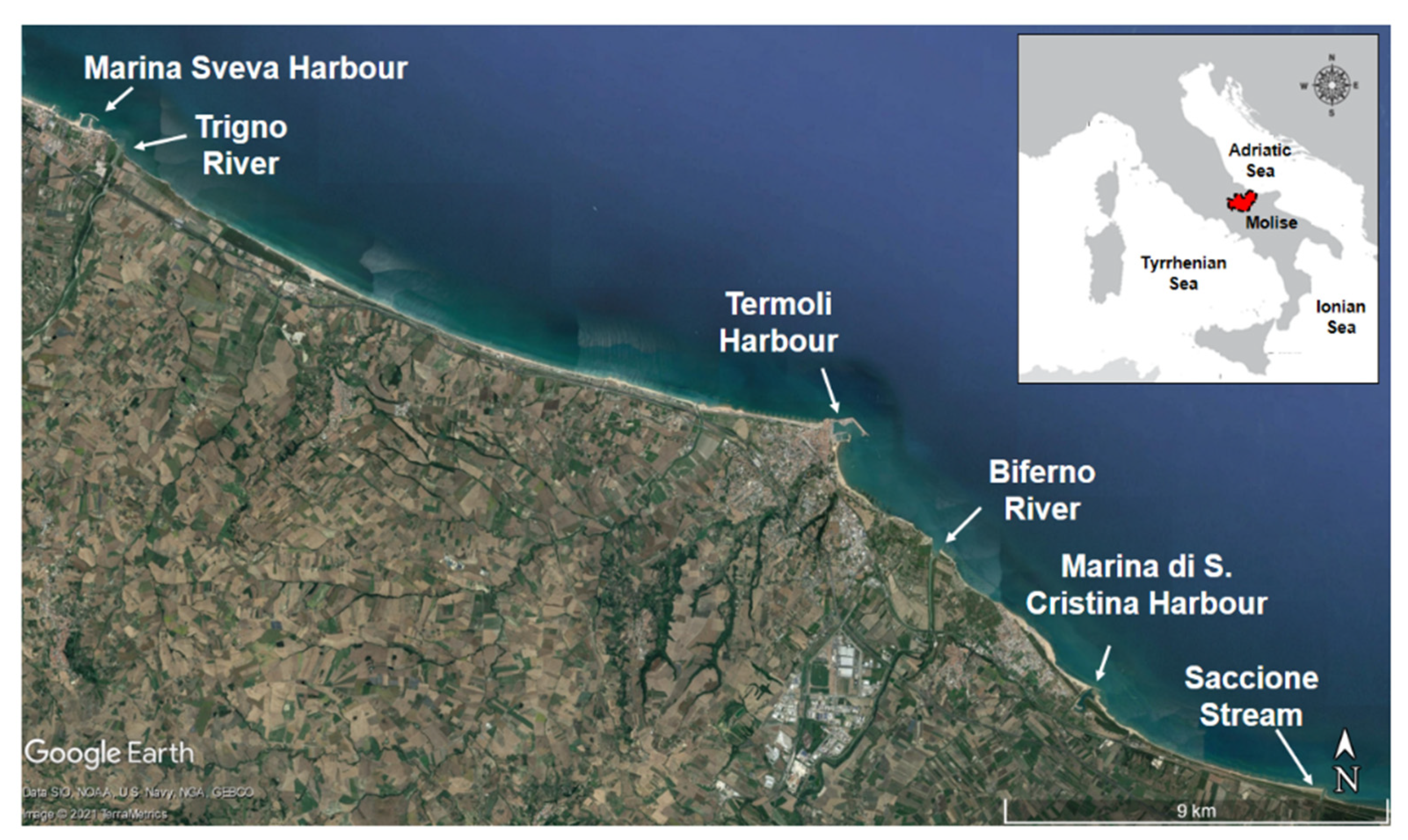
2. Regional Setting
2.1. Molise Coast and Shoreline General Trend
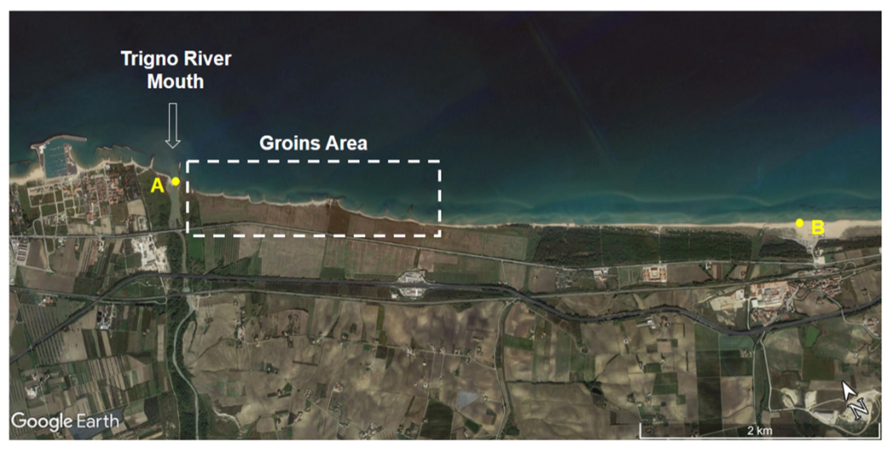
2.2. Trigno River Mouth
3. Materials and Methods
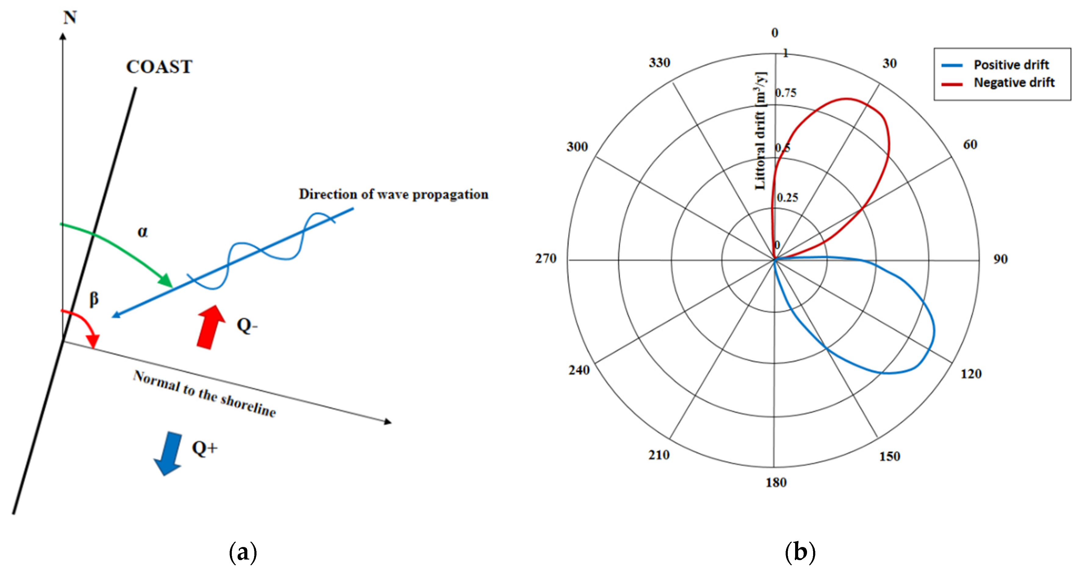
3.1. Littoral Drift Rose Concept and Shore Diffusivity
3.2. Wave Climate and Littoral Drift Rose of Molise Coast
3.2.1. Molise Wave Climate
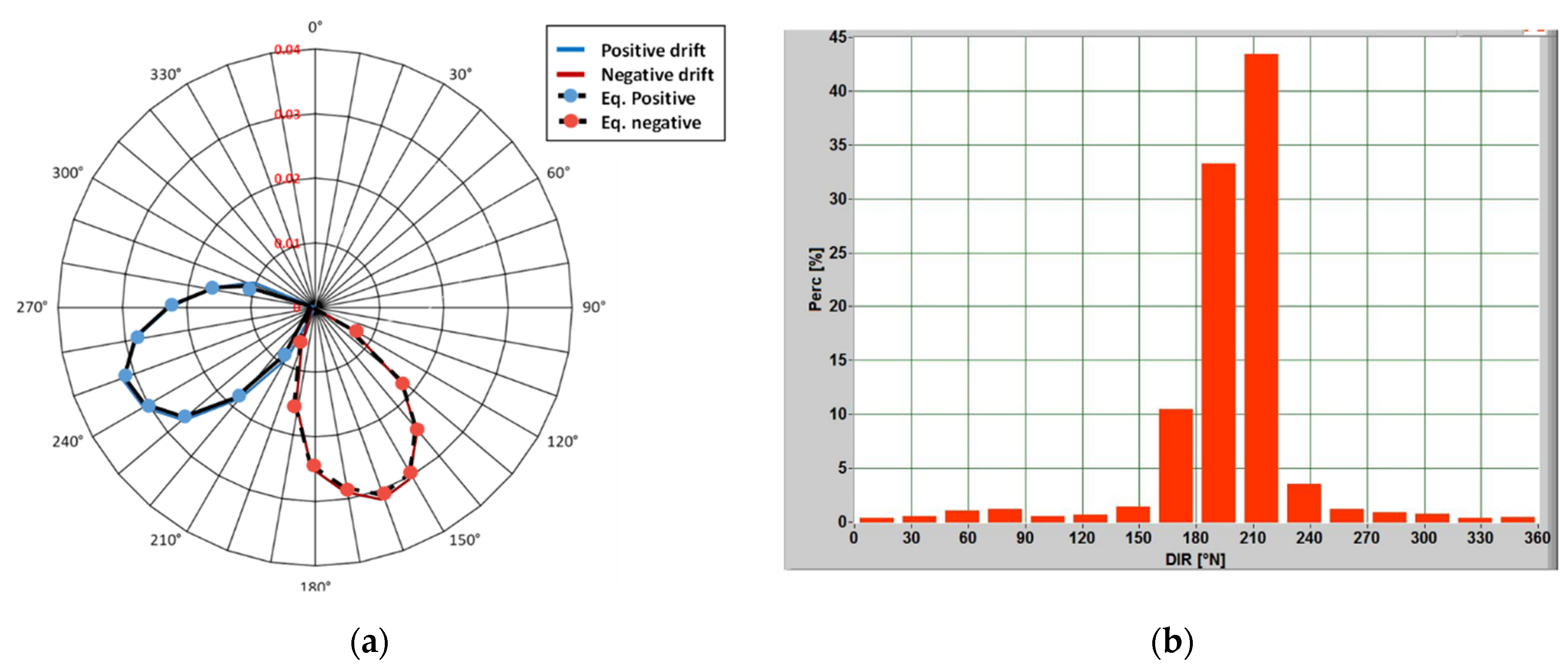
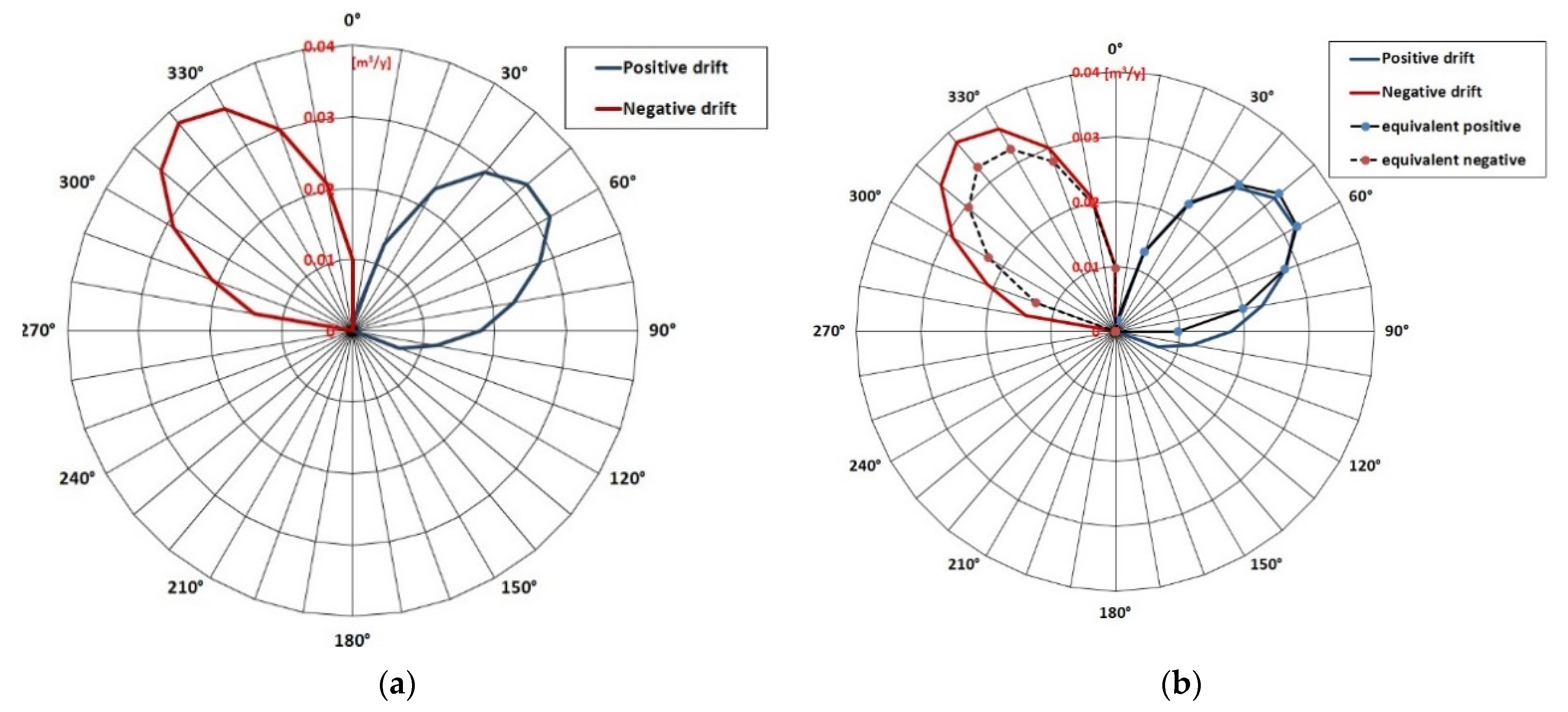
3.2.2. Molise LDR
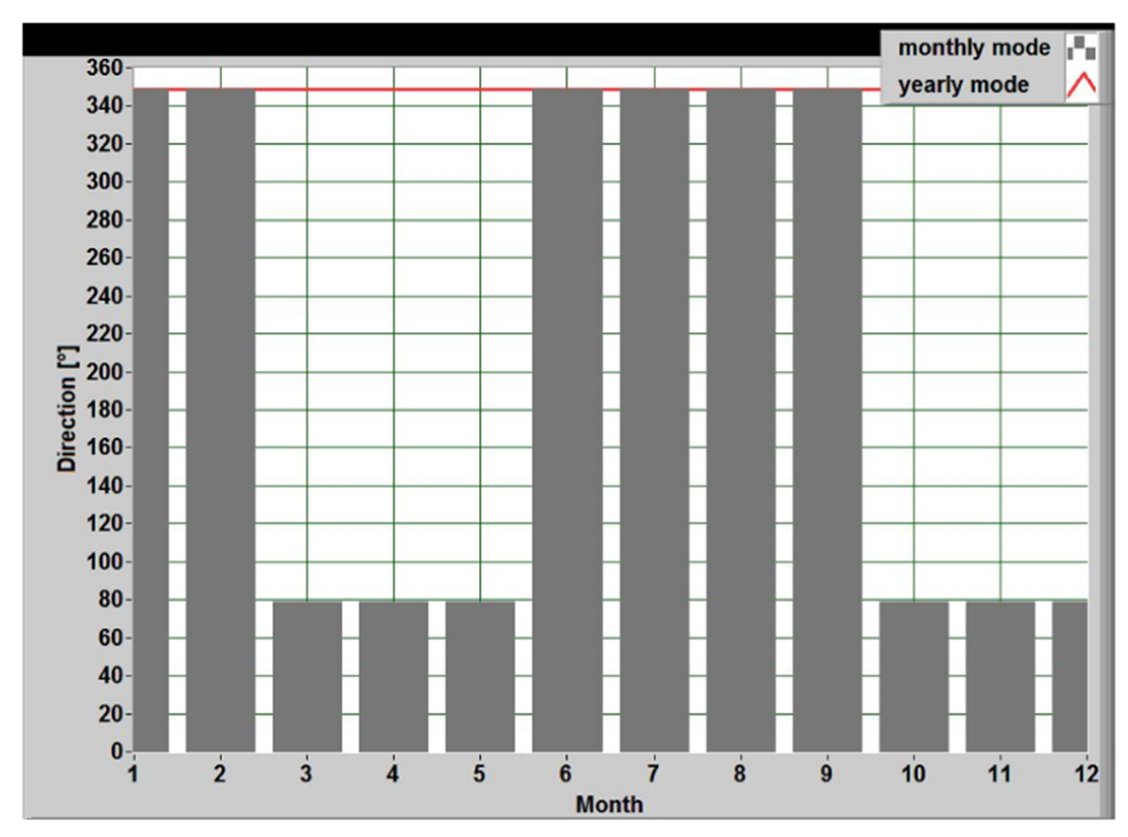
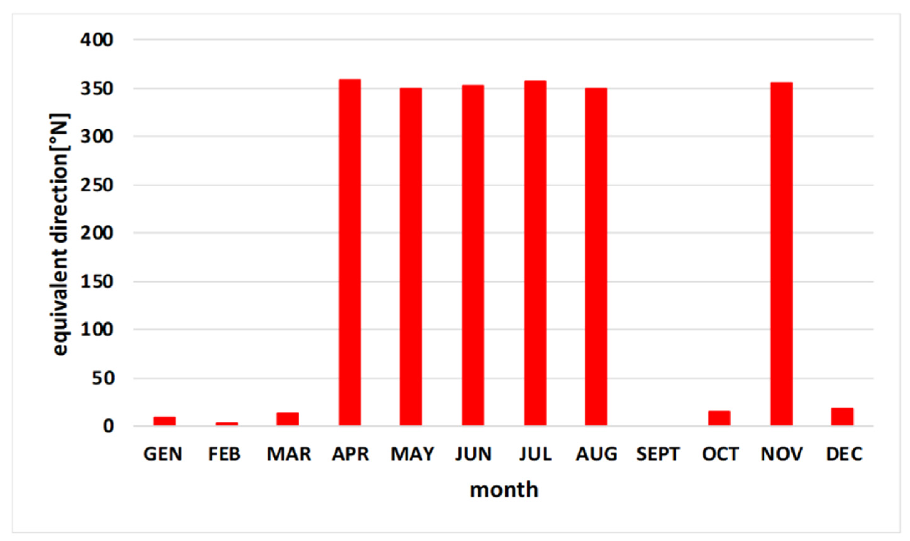
3.2.3. Monthly LDR-Equivalent Wave Climate
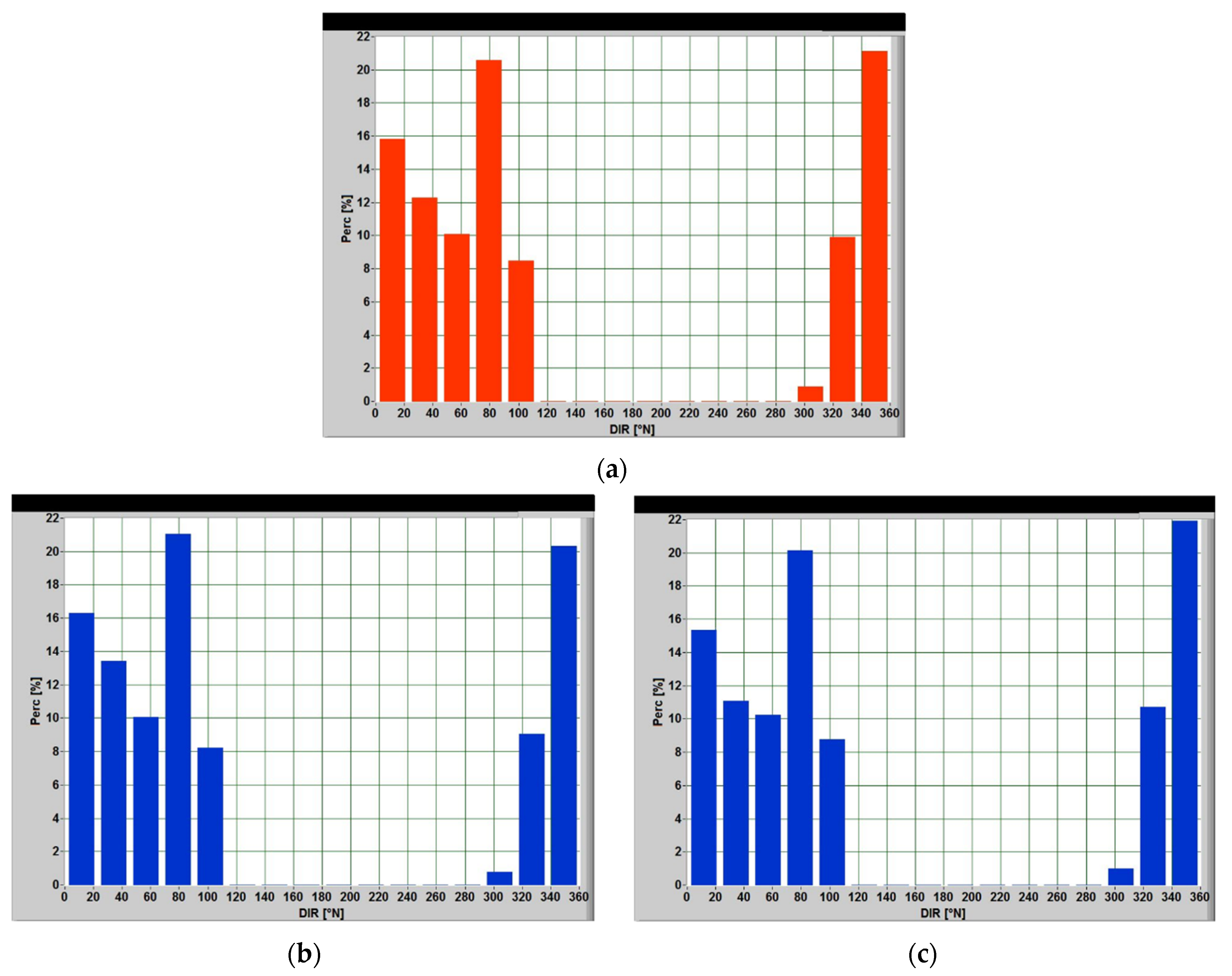
3.2.4. Frequency-Equivalent Wave Climate
3.3. Numerical Study
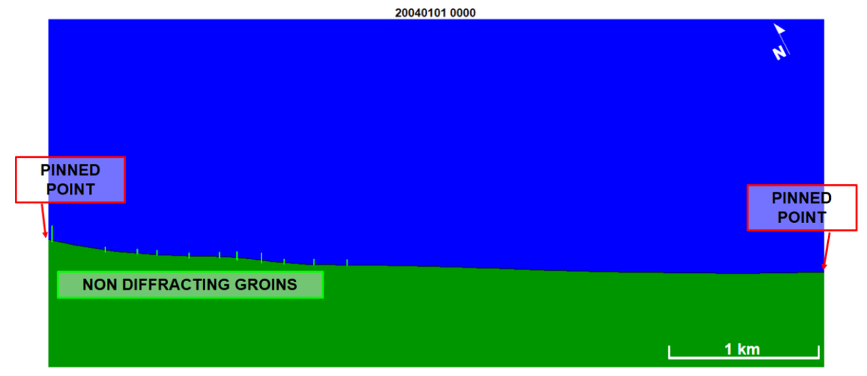
Software, Boundary Conditions and Model Parameters
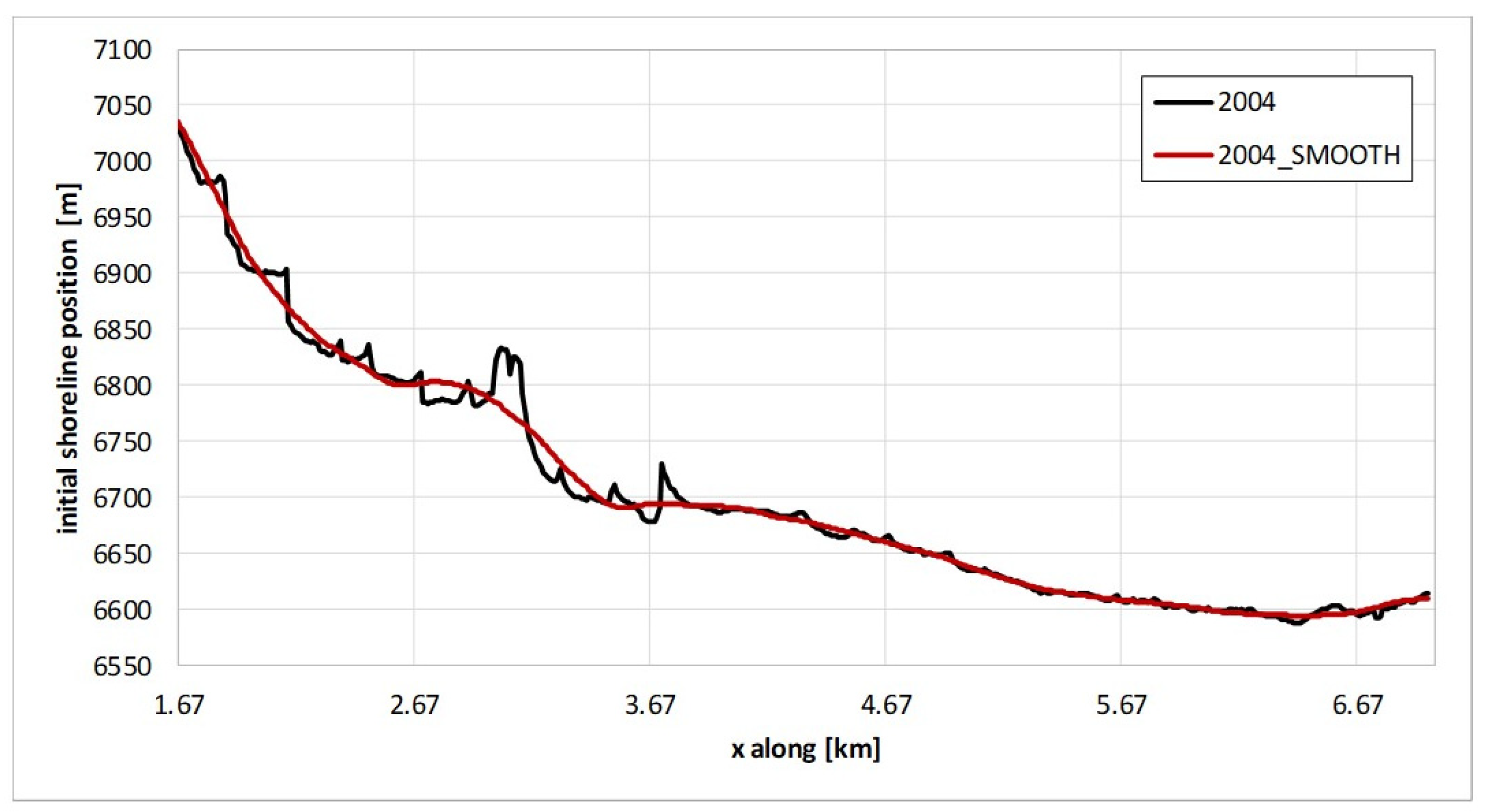
- Initial shoreline, y0 (x);
- Lateral boundary conditions;
- Structure characteristics;
- Transport coefficients;
- Values of Dc and DB;
- Wave climate.
4. Results
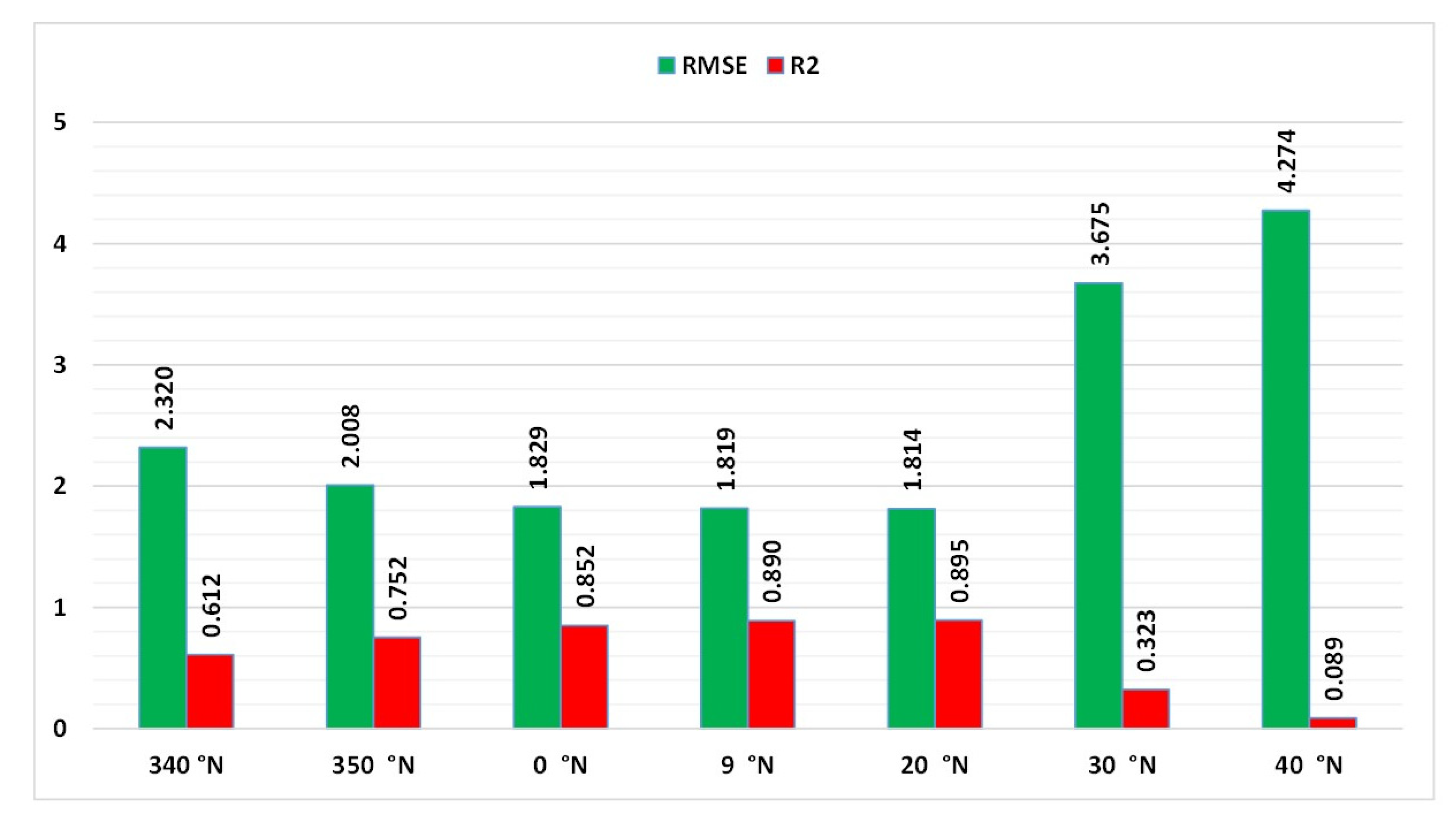
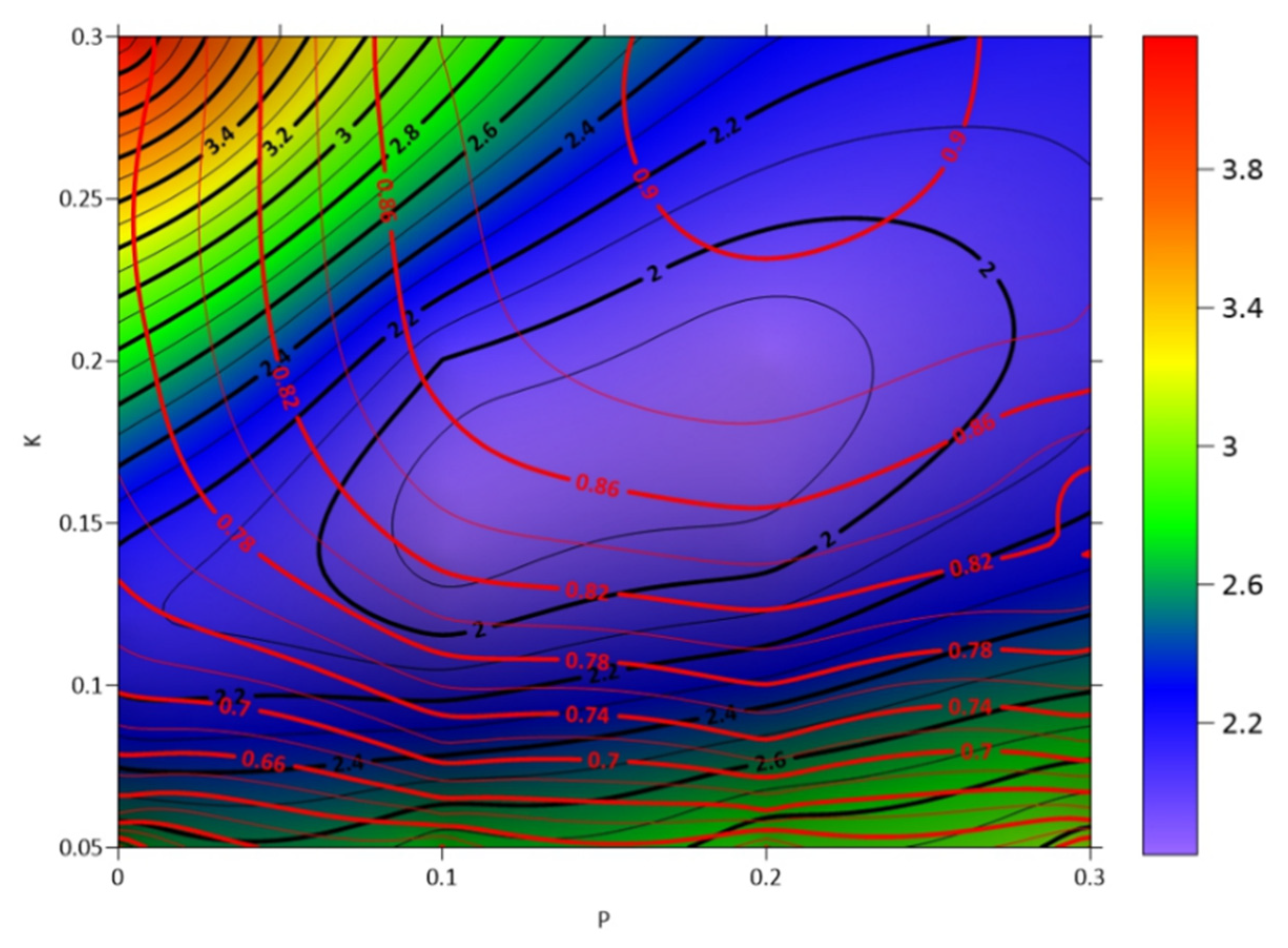
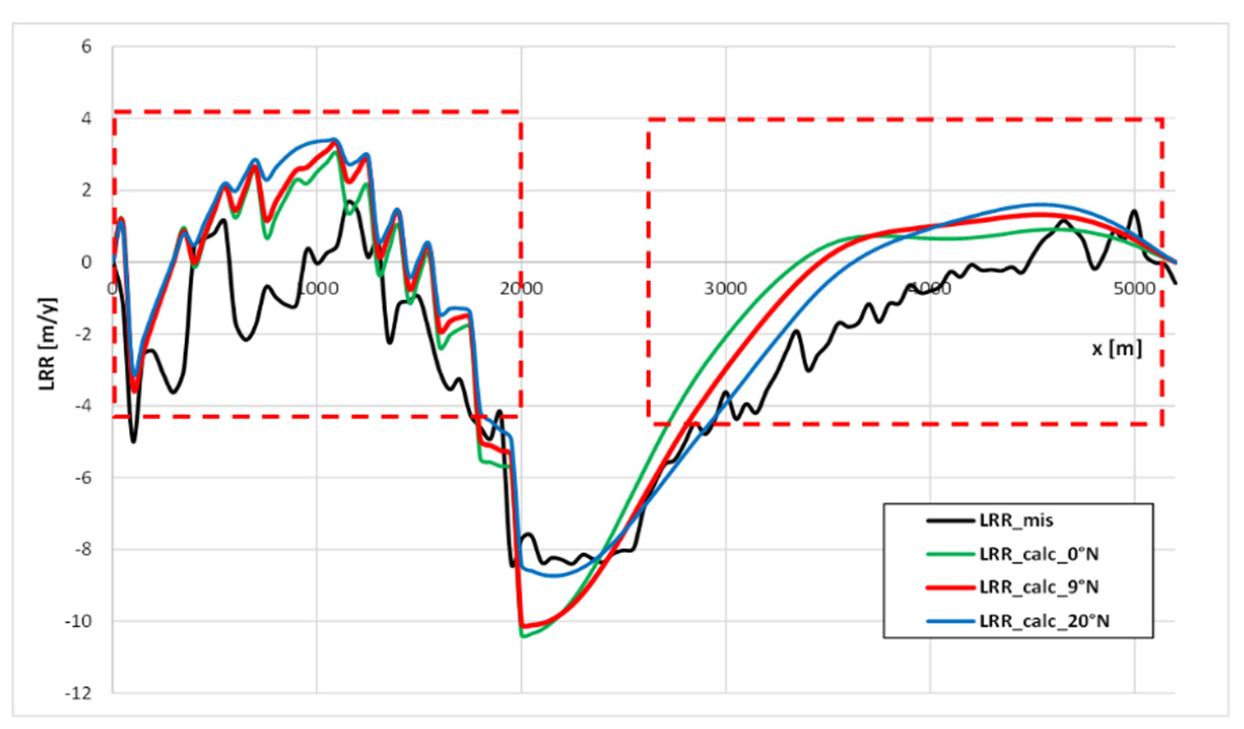
4.1. Annual LDR-Equivalent Wave Climate
- the R2 statistics, indicating the correlation between measured and predicted LRR;
- the relative mean square error (RMSE), given by
4.2. Monthly LDR-Equivalent Wave Climate
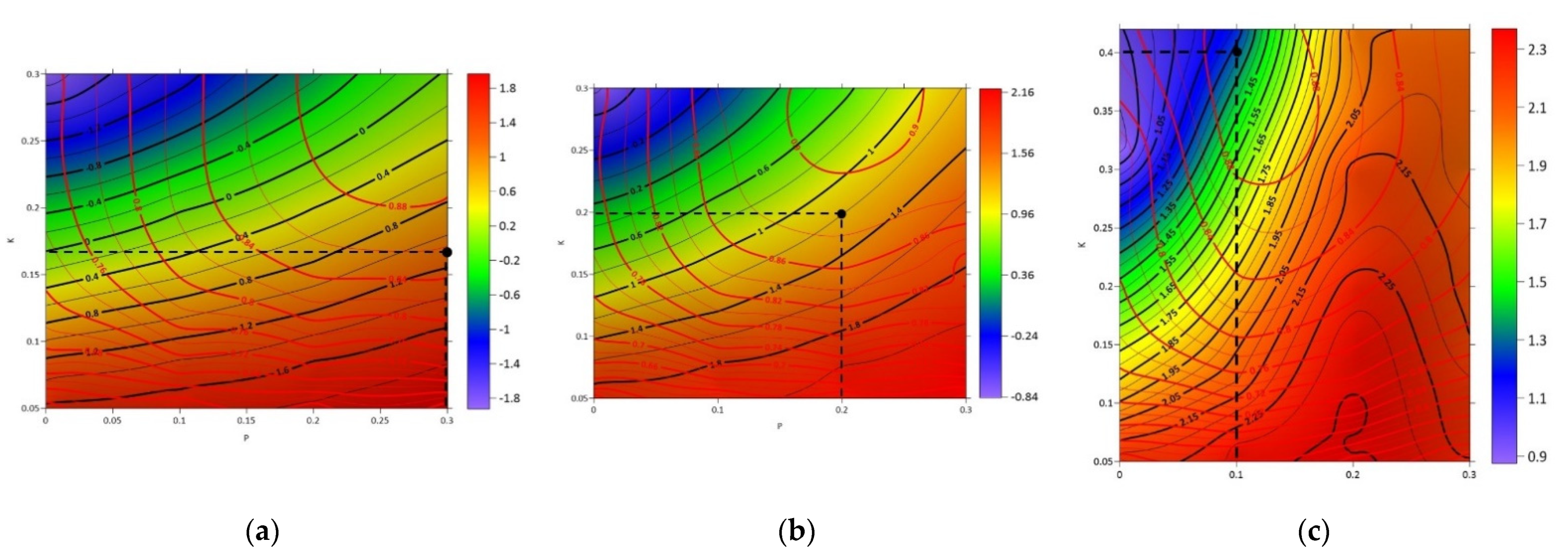
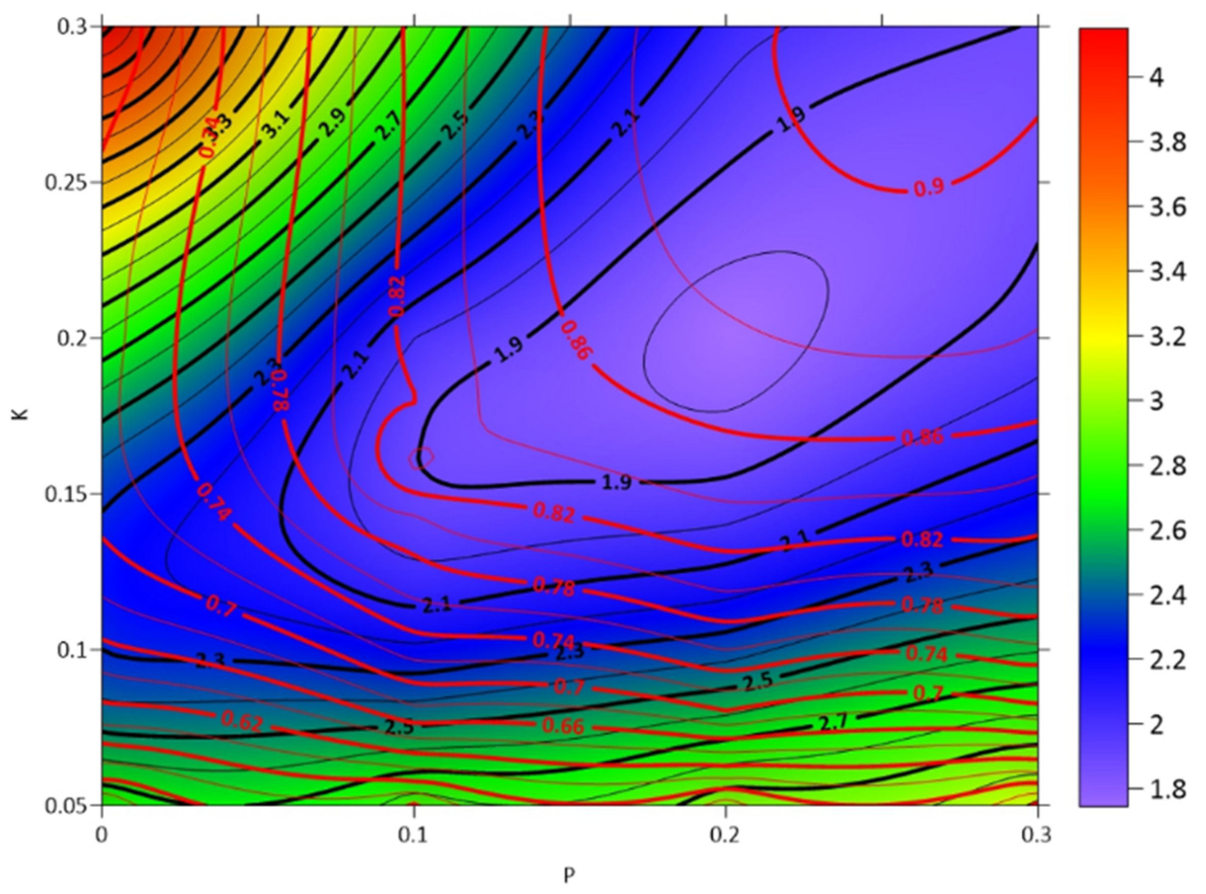
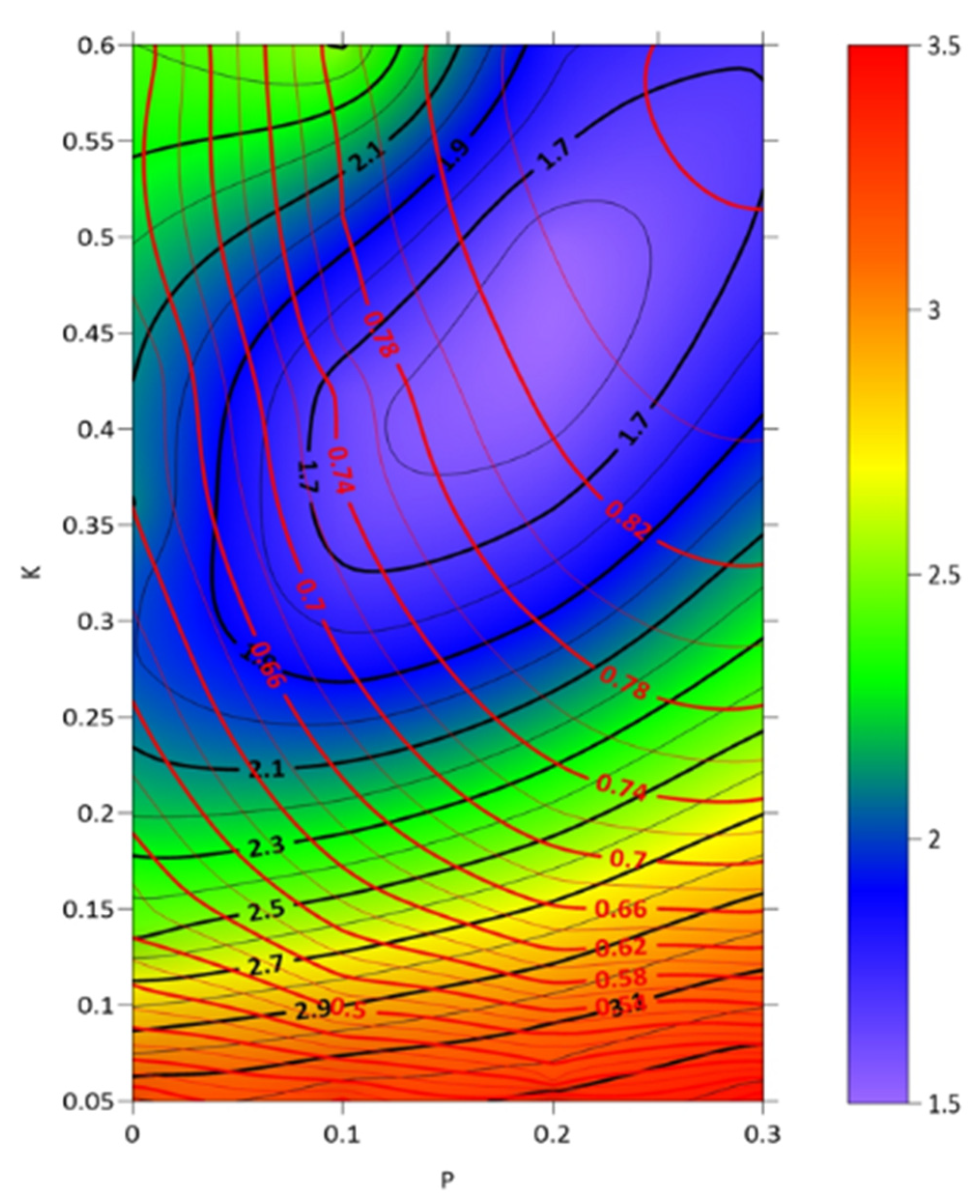
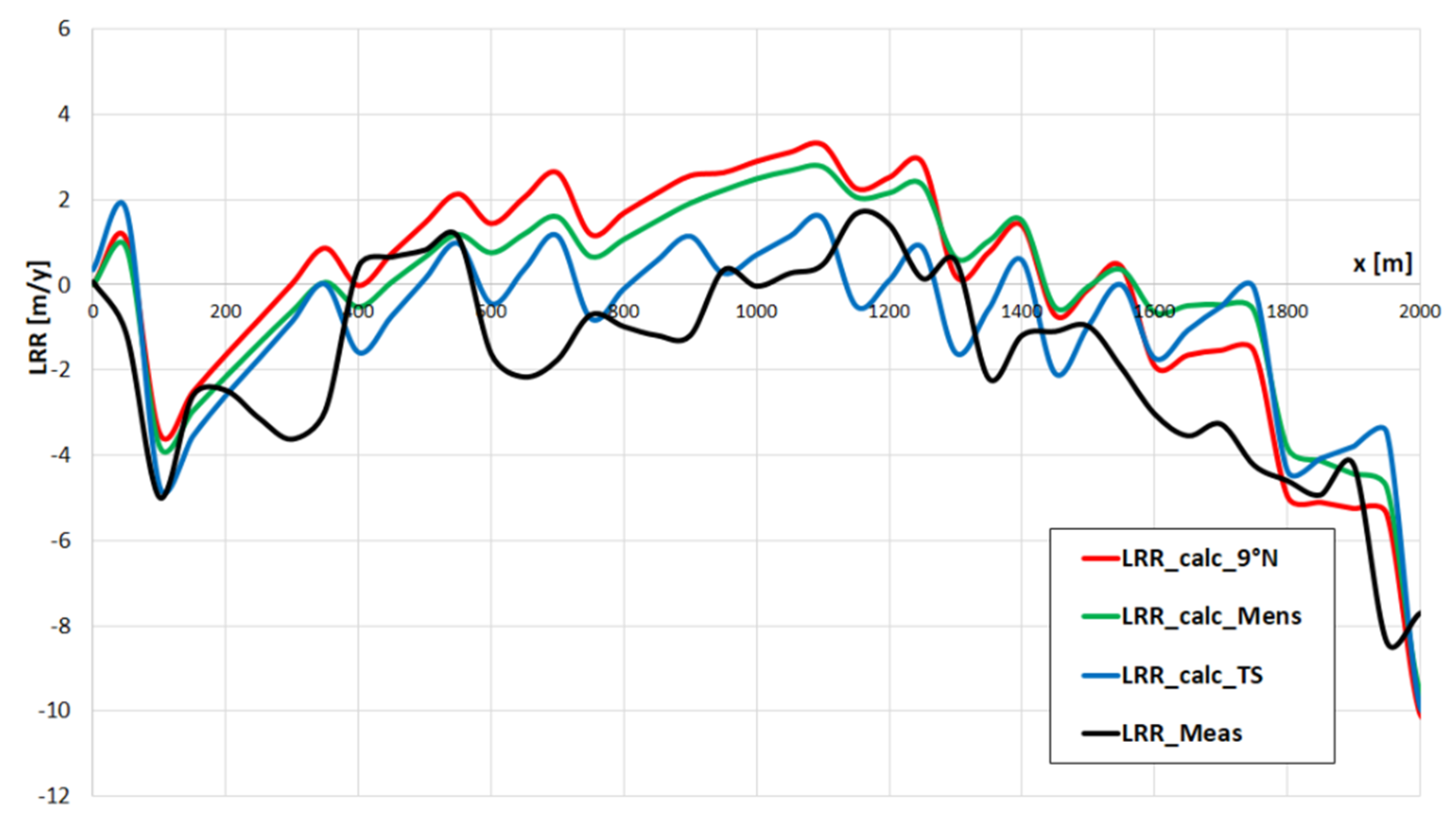
4.3. Frequency-Equivalent Time Series
5. Discussion and Conclusions
Author Contributions
Funding
Conflicts of Interest
References
- Hanson, H.; Kraus, N.C. GENESIS: A Generalized Shoreline Change Numerical Model for Engineering Use. Ph.D. Thesis, University of Lund, Lund, Sweden, 1989. [Google Scholar]
- Walton, T.L.; Dean, R.J. Application of Littoral Drift Roses to Coastal Engineering Problems. In Proceedings of the Conference on Engineering Dynamics in the Surf Zone, Institution of Engineers, Sydney, Australia, 14–17 May 1973; pp. 221–227. [Google Scholar]
- Walton, T.L.; Dean, R.J. Longshore Sediment Transport Via Littoral Drift Rose. Ocean. Eng. 2010, 37, 228–235. [Google Scholar] [CrossRef]
- Rosskopf, C.M.; Di Paola, G.; Atkinson, D.E.; Rodriguez, G.; Walker, I.J. Recent shoreline evolution and beach erosion along the central Adriatic coast of Italy: The case of Molise region. J. Coast. Conserv. 2018, 22, 879–895. [Google Scholar] [CrossRef]
- Aucelli, P.P.C.; Di Paola, G.; Rizzo, A.; Rosskopf, C.M. Present day and future scenarios of coastal erosion and flooding processes along the Italian Adriatic coast: The case of Molise region. Envrion. Earth Sci. 2018, 77, 371. [Google Scholar] [CrossRef]
- De Vincenzo, A.; Covelli, C.; Molino, A.J.; Pannone, M.; Ciccaglione, M.C.; Molino, B. Long-term Management Policies of Reservoirs: Possible Re-use of Dredged Sediments for Coastal Nourishment. Water 2019, 11, 15. [Google Scholar] [CrossRef] [Green Version]
- Molino, B.; Bufalo, G.; De Vincenzo, A.; Ambrosone, L. Semiempirical Model for Assessing Dewatering Process by Flocculation of Dredged Sludge in an Artificial Reservoir. Appl. Sci. 2020, 10, 3051. [Google Scholar] [CrossRef]
- Covelli, C.; Luigi, C.; Pagliuca, D.N.; Molino, B.; Pianese, D. Assessment of Erosion in River Basins: A Distributed Model to Estimate the Sediment Production over Watersheds by a 3-Dimensional LS Factor in RUSLE Model. Hydrology 2020, 7, 13. [Google Scholar] [CrossRef] [Green Version]
- Di Paola, G.; Ciccaglione, M.C.; Buccino, M.; Rosskopf, C.M. Influence of Hard Defence Structures on Shoreline Erosion Along Molise Coast (Southern Italy): A Preliminary Investigation. Rend. Online Ital. (ROL) 2020, 52, 2–11. [Google Scholar] [CrossRef]
- Buccino, M.; Di Paola, G.; Ciccaglione, M.C.; Rosskopf, C.M. A Medium-Term Study of Molise Coast Evolution Based on the One-Line Equation and “Equivalent Wave” Concept. Water 2020, 12, 2831. [Google Scholar] [CrossRef]
- Draper, N.R.; Smith, H. Applied Regression Analysis; John Wiley and Sons: Hoboken, NJ, USA, 1985. [Google Scholar]
- Aucelli, P.P.C.; Izzo, M.; Mazzarella, A.; Rosskopf, C.M.; Russo, M. L’evento meteorico estremo di gennaio 2003 sul Molise. Quad. Geol. Appl. 2004, 11, 101–119. [Google Scholar]
- Scorpio, V.; Aucelli, P.P.C.; Giano, S.I.; Pisano, L.; Robustelli, G.; Rosskopf, C.M.; Schiattarella, M. River channel adjustments in Southern Italy over the past 150 years and implications for channel recovery. Geomorphology 2015, 251, 77–90. [Google Scholar] [CrossRef]
- Aucelli, P.P.C.; Fortini, P.; Rosskopf, C.M.; Scorpio, V.; Viscosi, V. Recent channel adjustments and riparian vegetation response: Some examples from Molise (Italy). Geogr. Fis. Dinam. Quat. 2011, 34, 161–173. [Google Scholar] [CrossRef]
- Crowell, M.; Leatherman, S.P.; Buckley, M.K. Shoreline Change Rate Analysis: Long Term versus Short Term Data. Shore Beach 1993, 61, 13–20. [Google Scholar]
- US Army Corps of Engineers. Shore Protection Manual; Coastal Engineering Research Centre: Washington, DC, USA, 1984. [Google Scholar]
- Buccino, M.; Tuozzo, S.; Ciccaglione, M.C.; Calabrese, M. Predicting Crenulate Bay Profiles from Wave Fronts: Numerical Experiments and Empirical Formulae. Geosciences 2021, 11, 208. [Google Scholar] [CrossRef]
- Ashton, A.D.; Murray, A.B. High-angle wave instability and emergent shoreline shapes: 1. Modeling of sand waves, flying spits, and capes. J. Geophys. Res. 2006, 111, F04011. [Google Scholar] [CrossRef] [Green Version]
- Ashton, A.D.; Murray, A.B. High-angle wave instability and emergent shoreline shapes: 2. Wave climate analysis and comparisons to nature. J. Geophys. Res. 2006, 111, F04012. [Google Scholar] [CrossRef] [Green Version]
- Pelnard-Considere, R. Essai de theorie de l’evolution des forms de rivages en plage de sable et de galets. In 4th Journees de l’Hydralique, Les Energies De La Mer; Question III, Rapport No. 1; Société Hydrotechnique de France: Paris, France, 1956; pp. 289–298. [Google Scholar]
- Hallermeier, W.A. Field Data on Seaward Limit of Profile Change. J. Waterw. Port. Coast. 1985, 111, 598–602. [Google Scholar]
- Hasselmann, K.; Dunckel, M.; Ewing, J.A. Directional wave spectra observed JONSWAP. J. Phys. Oceanogr. 1973, 10, 1264–1280. [Google Scholar] [CrossRef]
- Contini, P.; De Girolamo, P. Impatto Morfologico di Opere a Mare: Casi di studio. In Proceedings of the VIII Conference Italian Association Offshore and Marina, La Spezia, Italy, 28–29 May 1998. [Google Scholar]
- Holthuijsen, L.H. Waves in Oceanic and Coastal Waters; University of Cambridge Press: Cambridge, UK, 2007. [Google Scholar]
- Buccino, M.; del Vita, I.; Calabrese, M. Predicting wave transmission past Reef Ball™ submerged breakwaters. J. Coast. Res. 2013, SI 65, 171–176. [Google Scholar] [CrossRef]
- N.W.H.; Bruce, T.; De Rouck, J.; Kortenhaus, A.; Pullen, T.; Schüttrumpf, H.; Troch, P.; Zanuttigh, B. 2018. Available online: www.overtopping-manual.com (accessed on 1 November 2018).
- Buccino, M.; Daliri, M.; Dentale, F.; Di Leo, A.; Calabrese, M. CFD experiments on a low crested sloping top caisson breakwater. Part 1. Nature of loadings and global stability. Ocean. Eng. 2019, 182, 259–282. [Google Scholar] [CrossRef]
- Buccino, M.; Daliri, M.; Dentale Calabrese, M. CFD experiments on a low crested sloping top caisson breakwater. Part 2. Analysis of plume impact. Ocean. Eng. 2019, 182, 345–357. [Google Scholar] [CrossRef]
- Hamm, L.; Peronnard, C. Wave parameters in the nearshore: A clarification. Coast. Eng. 1997, 32, 119–135. [Google Scholar] [CrossRef]


| Time Window | Average Shoreline Change (m/Year) |
|---|---|
| 1954–1986 | −1.52 |
| 1986–2016 | −2.02 |
| 1986–1998 | −0.61 |
| 1998–2011 | −1.94 |
| 2004–2016 | −2.33 |
| DD (°N) | P | K | RMSE (Months/Year) | R2 | μ (Months/Year) |
|---|---|---|---|---|---|
| 340 | 0.3 | 0.1 | 2.091 | 0.503 | 1.122 |
| 350 | 0.3 | 0.12 | 2.034 | 0.601 | 1.169 |
| 0 | 0.3 | 0.16 | 2.138 | 0.689 | 1.418 |
| 9 | 0.2 | 0.2 | 2.301 | 0.709 | 1.699 |
| 20 | 0.1 | 0.4 | 2.546 | 0.714 | 1.528 |
| 30 | 0 | 0.16 | 2.839 | 0.114 | 1.772 |
| 40 | 0.3 | 0.05 | 3.900 | 0.302 | 1.062 |
| P | K | R2 | RMSE (Months/Year) | μ (Months/Year) |
|---|---|---|---|---|
| 0 | 0.12 | 0.6841 | 2.248 | 1.23 |
| 0.1 | 0.16 | 0.8449 | 1.902 | 1.13 |
| 0.2 | 0.2 | 0.8766 | 1.743 | 1.20 |
| 0.3 | 0.2 | 0.9041 | 1.896 | 1.17 |
| P | K | RMSE (Months/Year) | R2 | μ (Months/Year) |
|---|---|---|---|---|
| 0 | 0.36 | 2.105 | 0.620 | 0.081 |
| 0.1 | 0.38 | 1.643 | 0.744 | 0.519 |
| 0.2 | 0.46 | 1.519 | 0.835 | 0.721 |
| 0.3 | 0.55 | 1.693 | 0.864 | 1.054 |
| Climate | P | K | RMSE (Months/Year) | R2 | μ (Months/Year) |
|---|---|---|---|---|---|
| Annual LDR (9° N) | 0.2 | 0.2 | 2.301 | 0.709 | 1.699 |
| Monthly LDR | 0.2 | 0.2 | 2.112 | 0.688 | 1.574 |
| Frequency EQ | 0.2 | 0.46 | 1.897 | 0.505 | 0.830 |
Publisher’s Note: MDPI stays neutral with regard to jurisdictional claims in published maps and institutional affiliations. |
© 2021 by the authors. Licensee MDPI, Basel, Switzerland. This article is an open access article distributed under the terms and conditions of the Creative Commons Attribution (CC BY) license (https://creativecommons.org/licenses/by/4.0/).
Share and Cite
Ciccaglione, M.C.; Buccino, M.; Di Paola, G.; Tuozzo, S.; Calabrese, M. Trigno River Mouth Evolution via Littoral Drift Rose. Water 2021, 13, 2995. https://doi.org/10.3390/w13212995
Ciccaglione MC, Buccino M, Di Paola G, Tuozzo S, Calabrese M. Trigno River Mouth Evolution via Littoral Drift Rose. Water. 2021; 13(21):2995. https://doi.org/10.3390/w13212995
Chicago/Turabian StyleCiccaglione, Margherita Carmen, Mariano Buccino, Gianluigi Di Paola, Sara Tuozzo, and Mario Calabrese. 2021. "Trigno River Mouth Evolution via Littoral Drift Rose" Water 13, no. 21: 2995. https://doi.org/10.3390/w13212995
APA StyleCiccaglione, M. C., Buccino, M., Di Paola, G., Tuozzo, S., & Calabrese, M. (2021). Trigno River Mouth Evolution via Littoral Drift Rose. Water, 13(21), 2995. https://doi.org/10.3390/w13212995