Evaluation of MNA in A Chlorinated Solvents-Contaminated Aquifer Using Reactive Transport Modeling Coupled with Isotopic Fractionation Analysis

Abstract

Groundwater contamination by chlorinated hydrocarbons is a worldwide problem that poses important challenges in remediation processes. In Italy, the Legislative Decree 152/06 defines the water quality limits to be obtained during the cleanup process. In situ bioremediation techniques are becoming increasingly important due to their affordability and, under the right conditions, because they can be more effective than conventional methodologies. In the initial feasibility study phase, the numerical modeling supports the reliability of each technique. Two different codes, BIOCHLOR and PHREEQC were discussed and compared assuming different field conditions. Isotopic Fractionation-Reactive Transport Models were then developed in one synthetic and one simple field case. From the results, the two codes were in agreement and also able to demonstrate the Monitored Natural Attenuation processes occurring at the dismissed site located in Italy. Finally, the PHREEQC model was used to forecast the remediation time frame by MNA, hypothesizing a complete source cleanup: a remediation time frame of about 10–11 years was achieved by means of natural attenuation processes.

1. Introduction

Chlorinated Hydrocarbons (CHCs) are globally distributed anthropogenic contaminants that affect the groundwaters at industrial sites. Tetrachloroethene (PCE), Trichloroethene (TCE) and Dichloroethene (DCE) were widely used in dry cleaning and degreasing operations, but had a large variety of other uses [1,2,3]. The Italian Legislative Decree 152/06, which adopts the European Directive 2006/118/CE, introduces the water quality objectives that must be fulfilled as a result of remediation processes, which correspond to the Contamination Concentration Threshold (CCT) for the different pollutants.

Nowadays, the in situ remediation methodologies for contaminated groundwaters are preferred because they avoid off-site handling of contaminated materials, resulting in less expensive operations [4]. Among these, bioremediation techniques are assuming more importance due to the relatively low costs and good removal efficiencies. Bioremediation involves the use of microorganisms to degrade the contaminants into non-harmful compounds; it can be divided into two main categories: Monitored Natural Attenuation (MNA), which is a passive methodology, and Enhanced Natural Attenuation (ENA), which involves active methodologies.

MNA is based on the reliance on natural processes to achieve site-specific remediation objectives within a time frame that is reasonable compared to that offered by other more active methods [5]. The key concepts of this method are to take advantage of preexisting processes occurring at the site and to benefit from the absence of direct actions on the contamination. The processes ascribable to natural attenuation are biodegradation, dispersion, dilution, volatilization, sorption, and biochemical stabilization. Among such processes, biodegradation plays an important role since it involves the reduction in contaminant mass, while the others involve dilution or sequestration processes. The knowledge and understanding of such processes, which are strictly related to the site-specific conditions, is essential to evaluate whether MNA can be a suitable methodology for the site remediation [6]; nevertheless, it requires a detailed site characterization aimed at the evaluation of the contaminant’s characteristics and the environment’s suitability for the natural attenuation processes [5]. The method minimizes the amount of material to be handled, mainly because all that are needed are the set-up of the observation wells and the simple monitoring of the concentration over time and the personnel exposure to the contaminations, resulting in a low-cost and safe method. For instance, considering the chlorinated solvents case, a common degradation pathway in reducing redox conditions is the reductive dechlorination, a bacteria-mediated process by Dehalococcoides strains [7,8]. In oxic conditions, a possible degradation pathway is provided by the cometabolic oxidation mediated by methanotrophic bacteria, even if it is reported to be significantly effective only in the plume fringe or along sections where the plume discharges to surface water bodies [4,9]. Compound Specific Isotope Analysis (CSIA) can improve MNA interpretation results [10,11,12,13,14,15], supporting the identification of the biodegradation processes and distinguishing them from other natural attenuation mechanisms, by means of the isotopic fractionation effect. However, many manuals and handbooks are present in the literature, encouraging the evaluation and the choice of MNA as a remediation strategy [5,16,17].

MNA is not accepted worldwide as a proper remediation technique, although its popularity is increasing, and more and more countries are including it in their national regulations on remediation processes. In the literature, [16,17] presented a comprehensive analysis of regulations in European countries and the USA, concerning MNA and the occurrence of this strategy as a remediation action. Countries such as the USA and the Flanders region in Belgium introduced MNA as a remediation strategy and often apply it, such as Germany does, but with the difference that is not yet clearly regulated. Finally, countries such as Finland do not recognize it as proper remediation action. However, MNA is generally coupled with other active remediation processes and usually is implemented for residual contaminations or low concentration plumes, mainly due to the quick response needed to protect sensible targets (e.g., a pump & treat procedure to protect water supply wells) that MNA is not able to fulfill.

Several case studies concerning the MNA approach applied alone or combined with other treatments are present: [18] applied the U.S. EPA’s screening protocol for MNA evaluation in the Superfund site of Brooklawn (Baton Rouge, LA, USA), where a CHC (chlorinated ethane and ethene compounds) contamination existed, highlighting the importance of implementing a detailed conceptual model. In the study, a Reactive Transport Model (RTM) through the U.S. EPA’s BIOCHLOR [19] was also developed and several simulations assuming different scenarios were performed, carrying out that MNA could be one of the feasible alternatives for the site remediation. In the literature, [4] presented the Twin Cities Army Ammunition Plant (TCAAP) case study (Arden Hills, MN, USA), where MNA was successfully applied to clean up the residual contamination by trichloroethene (TCE) and 1,1,1-tichloroethane (1,1,1-TCA) after the application of active remediation strategies (pump & treat, P&T). Additionally, [20] presented the unique Italian case study available in the literature, showing evidence of degradation by natural attenuation for a BTEXS plume in the NIT site and highlighting the need for evaluation protocols before the application of this methodology in formal plans. Some studies include a comprehensive analyses of several plumes managed through MNA [21,22], other studies on Carbon Tetrachloride and Chloroform plume [23], CHCs [24,25,26,27], and hydrocarbons [28,29,30] and abiotic MNA [31].

Numerical modeling enables evaluation and prediction of the results of MNA and ENA approaches: some numerical codes can be applied with this goal and the purpose of the code selection is to identify appropriate models to develop an Isotopic Fractionation-Reactive Transport Model (IF-RTMs) able to simulate MNA or ENA processes. In the literature, a variety of codes are able to reproduce reactive transport conditions is present [32,33,34,35]. Some implement analytical solutions, such as BIOCHLOR [19] and BIOSCREEN [36], while others are numerical codes, such as PHREEQC [37], PHT3D ([38,39,40,41], which is a code coupling PHREEQC and MT3D [42] a solute transport code based on a MODFLOW [43]), RT3D [44], OpenGeoSys [45,46], TOUGHREACT [47], MIN3P [48,49,50] and many others. However, not all the codes can simulate the isotopic fractionation (IF), e.g., BIOCHLOR-ISO [51,52] and PHREEQC. BIOCHLOR-ISO is an extension of the EPA’S BIOCHLOR, an analytical model able to reproduce both the natural attenuation processes and the isotopic fractionation occurring during biodegradation through an extension of the analytical solution proposed by [53]; the codes also include the stable isotope ratios analysis for carbon and chlorine isotopes in chloroethenes [54,55]. BIOCHLOR-ISO exists in a version that considers only carbon isotopes (2015 version, [51]) and a more recent version where the dual-isotope approach (carbon-chlorine, version 2016, [52]) is implemented. PHREEQC is a 1D geochemical code that allows the definition of customized reactions defining any type of compound as a new chemical species. Such versatility makes PHREEQC a simple numerical model able to reproduce many possible situations occurring in the groundwater. In the literature, many examples of RTMs implemented by means of PHREEQC are discussed. In [56], an IF-RTM for a chlorinated ethenes plume is presented, while [57] discussed a model able to reproduce 3D-CSIA data. Beyond CHCs, PHREEQC, for example, was used to simulate behavior of arsenic in groundwater [58,59,60,61,62], the behavior of soluble reactive phosphorus [63], to model carbon and hydrogen isotopes during propanol and toluene volatilization [64], heavy metal dissolution [65] and to simulate electrokinetic transport and biogeochemical reactions in porous media [66].

Nowadays, it is becoming clear that RTMs and CSIA are important tools for the assessment of bioremediation processes that can help Public Authorities in accepting MNA as remediation strategy. Indeed, the combination of these tools can strengthen the confidence of designers and controllers in the existence of active biodegradation processes, allowing a better evaluation of the feasibility and design of remediation actions. For this reason, it is needed to perform field-case studies in which these tools are applied.

In the present study, the analytical and numerical codes that are suitable for modeling both the reactive transport and the isotopic fractionation (IF-RTM) reproducing the natural attenuation processes were initially selected. Then, an initial comparison between the numerical code (PHREEQC) and the analytical one (BIOCHLOR) was carried out, in order to further validate the first code.

The aim of this study is to evaluate the feasibility of MNA as remediation strategy in a real dismissed contaminated site in southern Italy by means of data interpretation and numerical modelling, in order to demonstrate the advantages of the combined application of RTMs and CSIA. First, a CSM was developed and then a numerical model was implemented both for descriptive and forecast purposes. After an initial calibration of the degradation parameters, the numerical model was used to forecast the remediation time frame as a result of the removal of the pollution source.

2. Materials and Methods

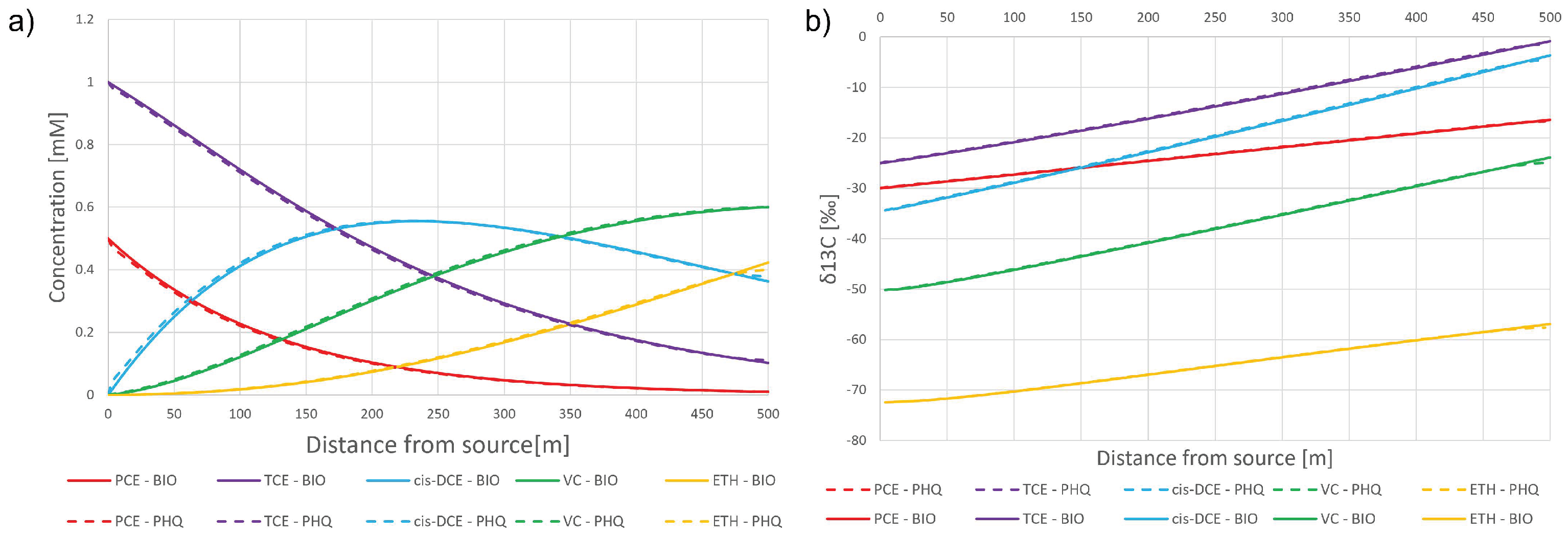
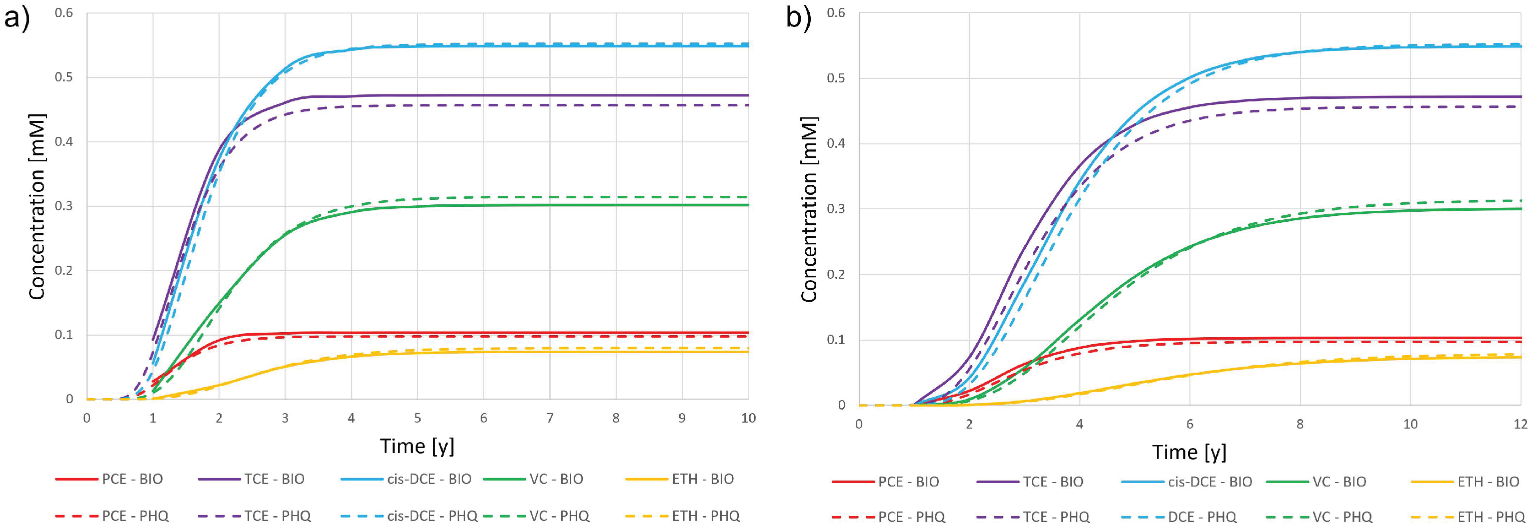
PHREEQC was selected as the IF-RTM numerical code, as it was deemed suitable to represent the 1D conditions of the site and BIOCHLOR-ISO was selected as the analytical code since it is a well-established tool to evaluate the MNA processes. The MNA is strongly based upon a full conceptual model, borehole drillings, monitoring and characterization of the polluted site; however, a preliminary analysis carried out by means of numerical models can be useful to understand the feasibility of the approach.

2.1. Synthetic Case

The first step of this study was to compare the results of PHREEQC and BIOCHLOR-ISO for a benchmark case, concerning a groundwater contamination by chlorethenes. In accordance with the example discussed in [51] based on the work of [67], PHREEQC codes were developed (the code is provided as Supplementary file S4) for two different cases, summarized in

Table 1. Comparison case summary.

Case	RTM 1	Sorption	IF 2
Case 1	✓	✗	✓
Case 2	✓	✓	✗

¹ RTM = Reactive Transport Model; ² IF = Isotopic Fractionation.

. Since PHREEQC can simulate only 1D transport, the benchmark example was modified to compare the results by setting the transversal parameters (transversal and vertical dispersion) to 0 and the source dimensions equal to unity. The simulation ran for 30 years to reach steady-state conditions. A summary of the model parameters used in each case is presented in the Supplementary Materials (Table S1).

The two versions of BIOCHLOR-ISO give the same results for the IF-RTM simulations, while BIOCHLOR-ISO version 2015 is not able to model the solute sorption; therefore, for Case 2 only BIOCHLOR-ISO version 2016 was used. The parameters used in the BIOCHLOR-ISO model are provided in Supplementary file S1. A comprehensive User’s Guide for BIOCHLOR-ISO version 2015 is reported as Supplementary file S2. The models developed in PHREEQC need more inputs. First, the chemical species (which are PCE, TCE, DCE and VC) must be defined through the KEYWORDS (specific word of the programming language that defines an internal algorithm in PHREEQC code) “SOLUTION_MASTER_SPECIES” and “SOLUTION_SPECIES”, assigning a name to each of them. For a detailed description of the code and KEYWORDS, see the Supplementary file S4. Second, the initial concentration in each cell at the boundary side (concentrations of the four compounds, called “infilling solution”) is defined by the keyword “SOLUTION”. Third, through “KINETICS”, the stoichiometry and the degradation parameters needed in the calculations must be defined. Fourth, the degradation reactions must be specified: e.g., assuming a 1:1 stoichiometry for each time step, the model calculates, a certain amount of 1,2-cis-DCE produced by the degradation of its parent compound (TCE) and a certain amount of degraded 1,2-cis-DCE, which becomes its daughter compound (VC). This behavior can be modeled following a first order degradation sequential process, as described in [19].

The concentration of a generic compound i, at a given time t, for a known initial concentration $C\left(t=0\right)$, is given by the negative exponential:

$$C_i\left(t\right)=C_i\left(t=0\right)e^{-{\lambda }_{i}t}$$

(1)

where ${\lambda }_i$ is the degradation rate constant of the related compound. The keyword “RATE” defines a reaction for each compound, through a Basic code. The code reads the moles of each compound present in the cell, then reads the degradation parameter from the “KINETICS” keyword and calculates the increase/decrease in moles (depending on the sign defined in the stoichiometry) in the specific time step integrating the equation in time.

Finally, by means of the “TRANSPORT” keyword, the usual groundwater flow and transport parameters are defined.

In Case 1, a more complex code was written because of the presence of different isotopic species. Indeed, the “heavy” and the “light” isotope of each compound must be defined as a separate chemical species to carry out the calculations. The initial concentration of the two isotopes can be calculated from the initial isotopic composition, assuming that the sum of the two carbon (C) isotopes gives the total amount of C:

$${}_{ }{}^{12}C=C-{}_{ }{}^{13}C$$

(2)

$$R_{comp}=\frac{{}_{ }{}^{13}C}{{}_{ }{}^{12}C}=\frac{{}_{ }{}^{13}C}{C-{}_{ }{}^{13}C}$$

(3)

$${\delta }^{13}C=\left(\frac{R_{comp}}{R_{STD}}-1\right)\times 1000$$

(4)

where ${}_{ }{}^{13}C$ and ${}_{ }{}^{12}C$ are the concentrations (in $\mathrm{mol}/\mathrm{l}$) of the heavy and light C isotope, respectively, $R_{comp}$ is the isotopic ratio, $R_{STD}$ is the standard isotopic ratio (Vienna Pee Dee Belemnite, shortened as VPDB, 0.0112372), and ${\delta }^{13}C$ is the isotopic signature.

Next, because the reaction rates change from light to heavy isotope (slower for the last one), the equations must be adapted. First, in KINETICS, the reaction rate is provided for the light isotope species and the enrichment factor (ε) is provided for the heavy one. Then, the equations are written for the two isotopes (modified from [56]).

$$\delta {}_{ }{}^{12}C=[{\lambda }_i\times {}_{ }{}^{12}C]\times t$$

(5)

$$\delta {}_{ }{}^{13}C={\alpha }_i\times [{\lambda }_i\times {}_{ }{}^{13}C]\times t$$

(6)

where, for a generic compound $i$, ${}_{ }{}^{13}C$ and ${}_{ }{}^{12}C$ are the concentrations (in $\mathrm{mol}/\mathrm{l}$) of the heavy and light C isotope, respectively, ${\lambda }_i$ is the degradation rate constant, ${\alpha }_i$ is the fractionation factor, and $t$ is the time. Finally, the isotopic composition is calculated through Equation (4) once the abundance of the two isotopes is known.

In Case 2, sorption mechanisms were considered. Assuming a linear isotherm, the sorption effect was modeled through the introduction of a retardation factor $(R_d)$, calculated as:

$$R_d=1+\frac{{\rho }_b}{\theta }\times f_{oc}\times k_{oc}$$

(7)

where ${\rho }_b$ is the bulk density (g/cm³), $\theta$ is the porosity, $f_{oc}$ is the fraction of organic carbon and $k_{oc}$ is the partition coefficient (cm³/g). The product $f_{oc}\times k_{oc}$ is often indicated as $K_d$ (distribution coefficient).

The BIOCHLOR-ISO 2016 solution only allows the application of an overall retardation factor ($R_{d,model}$), which was calculated as the average value of all components, since each compound has its specific retardation factor depending on the partition coefficient ($k_{oc}$). To compare the PHREEQC results with the BIOCHLOR-ISO 2016 ones, the overall retardation factor was applied to both the seepage velocity ($v_r$) and the degradation rate constants (${\lambda }_i$). Therefore, the retarded velocity $v_{ret}$ and the new degradation rate constants (${\lambda }_{i,ret}$) were computed as:

$$v_{ret}=\frac{v_r}{R_{d,model}}$$

(8)

$${\lambda }_{i,ret}=\frac{{\lambda }_i}{R_{d,model}}$$

(9)

2.2. Field Case

The codes were then applied to a real case study, representing an industrial site in southern Italy. The plant started its activity in the early 1960s, remaining in production until 1979 when the activities ceased. During this period, the plant produced VCM/PVC (Monomer Vinyl Chloride and Poly Vinyl Chloride), methanol, and caustic soda. At the beginning of the 1990, all the industrial facilities were demolished, and a first site characterization of the soils and groundwater was carried out. Then, a groundwater monitoring program was activated, and a large number of concentration data of the pollutants was collected, evidencing the current presence of a secondary source composed by TCE, 1,2-cis-DCE and VC. However, based on the historical production information, the primary source was probably caused by a TCE storage facility. Among the different contaminants present in the area, the chlorinated ethenes were the most diffused and therefore were studied in detail. In particular, the conceptual model implemented in the numerical codes concerns the NE side of the site, where the contaminant’s plume is well detected by a series of monitoring wells displaced along the natural groundwater flow direction (Figure 1b), running along a slurry wall.

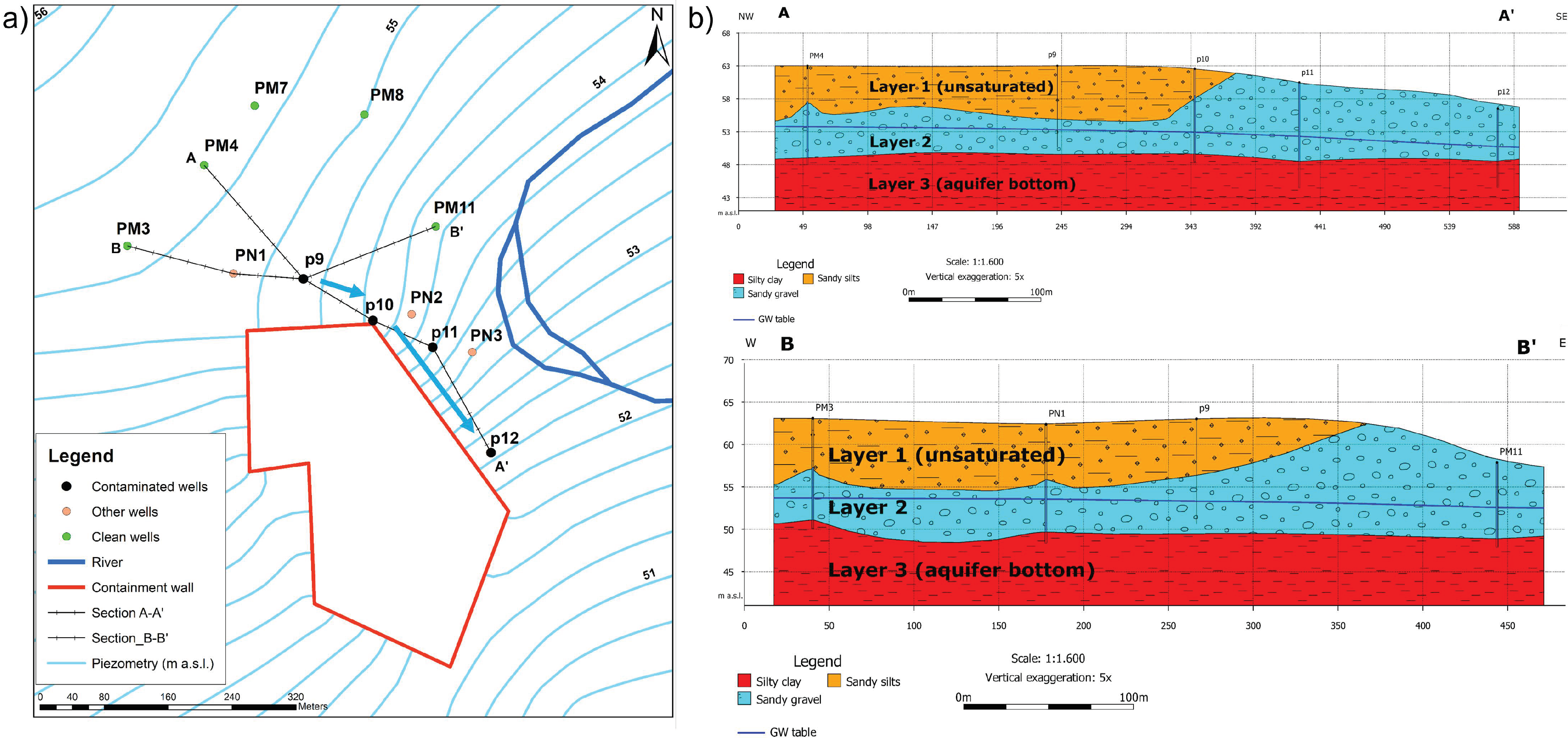
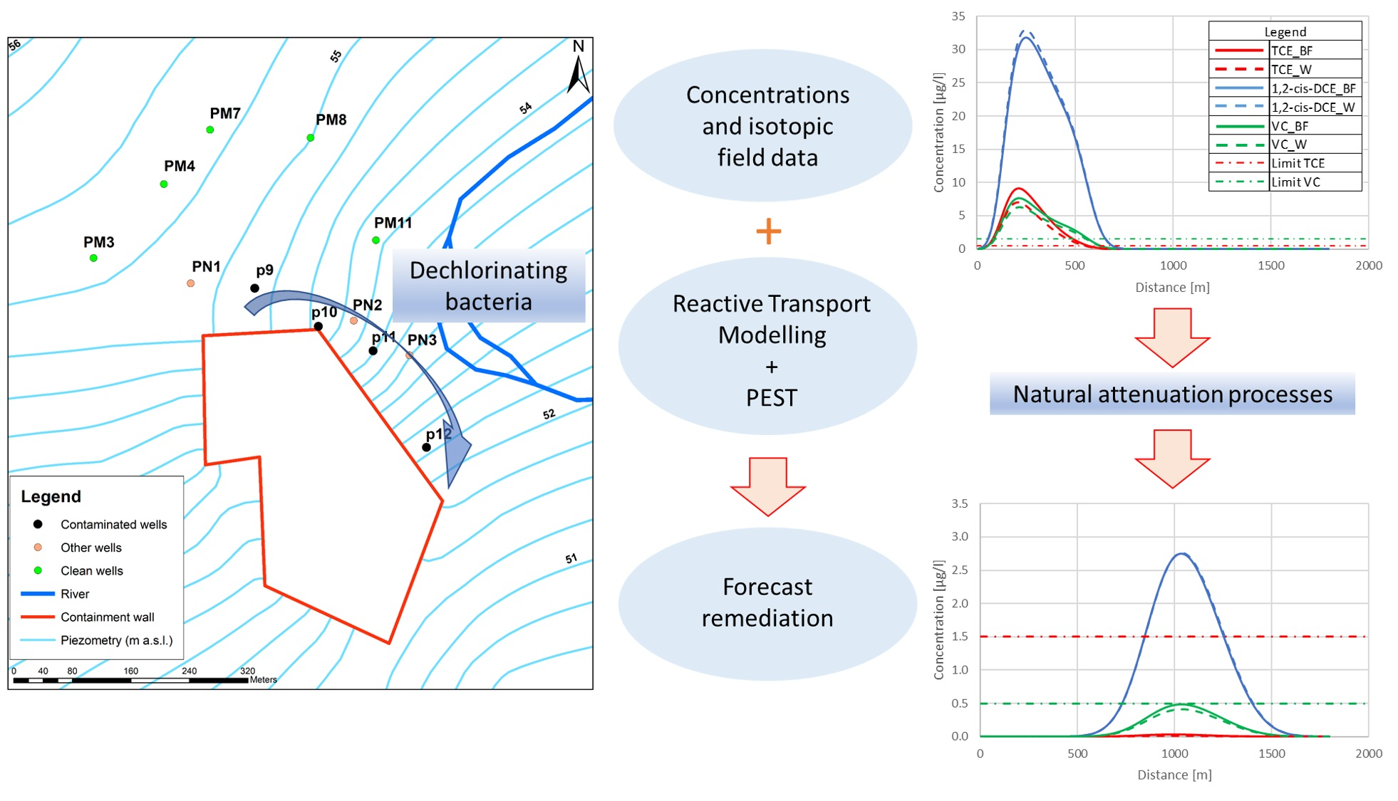
2.2.1. Hydrogeological Setting

The site is located in a valley and has a river to the east, in a fairly flat area. The geology is characterized almost completely by quaternary and recent alluvial deposits in the valley floor, while argillites have emerged on the sides, creating a low permeability boundary. The characterization surveys identified three different stratigraphic layers, as already shown in [68] (Figure 1a):

• Sandy silts: consisting of recent Holocenic alluvial sediments, this layer is composed of sandy silts and silty fine sands, with an average thickness of 5 m. The hydraulic conductivity was derived from an in situ pumping test and estimated to be around 10⁻⁷ m/s. This layer is unsaturated.
• Sandy gravels: also consisting of recent Holocenic alluvial sediments, this layer is composed of polygenic gravels with sub-rounded clasts in sandy or silty sandy matrix. The hydraulic conductivity of the layer was derived from an in situ pumping test and estimated to be around 10⁻⁴ m/s. This layer hosts the phreatic aquifer that is characterized by a saturated thickness between 3 m and 5.30 m; the total thickness of the layer in the area is about 5–10 m.
• Silty clay: consisting of Pliocenic sediments, this layer reaches considerable thickness (greater than 50 m). This is considered the bottom of the aquifer (low permeability boundary), since is consisting of not permeable alluvial materials with a hydraulic conductivity estimated (from literature analyses) around 10⁻⁸–10⁻¹¹ m/s.

The groundwater flow is mainly from NO towards SE, with an average hydraulic gradient of 0.005 and an average hydraulic conductivity of about 5 × 10⁻⁴ m/s.

Locally, the piezometric map shows that the water runs along the containment wall turning southwards in correspondence of the piezometer p10, flowing towards p11 and p12. Globally, in the area, groundwater table distance from the ground surface varies from 5 (upgradient of the wall) to 10.5 m.

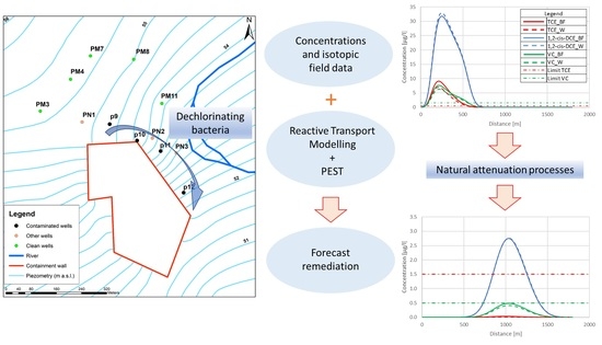
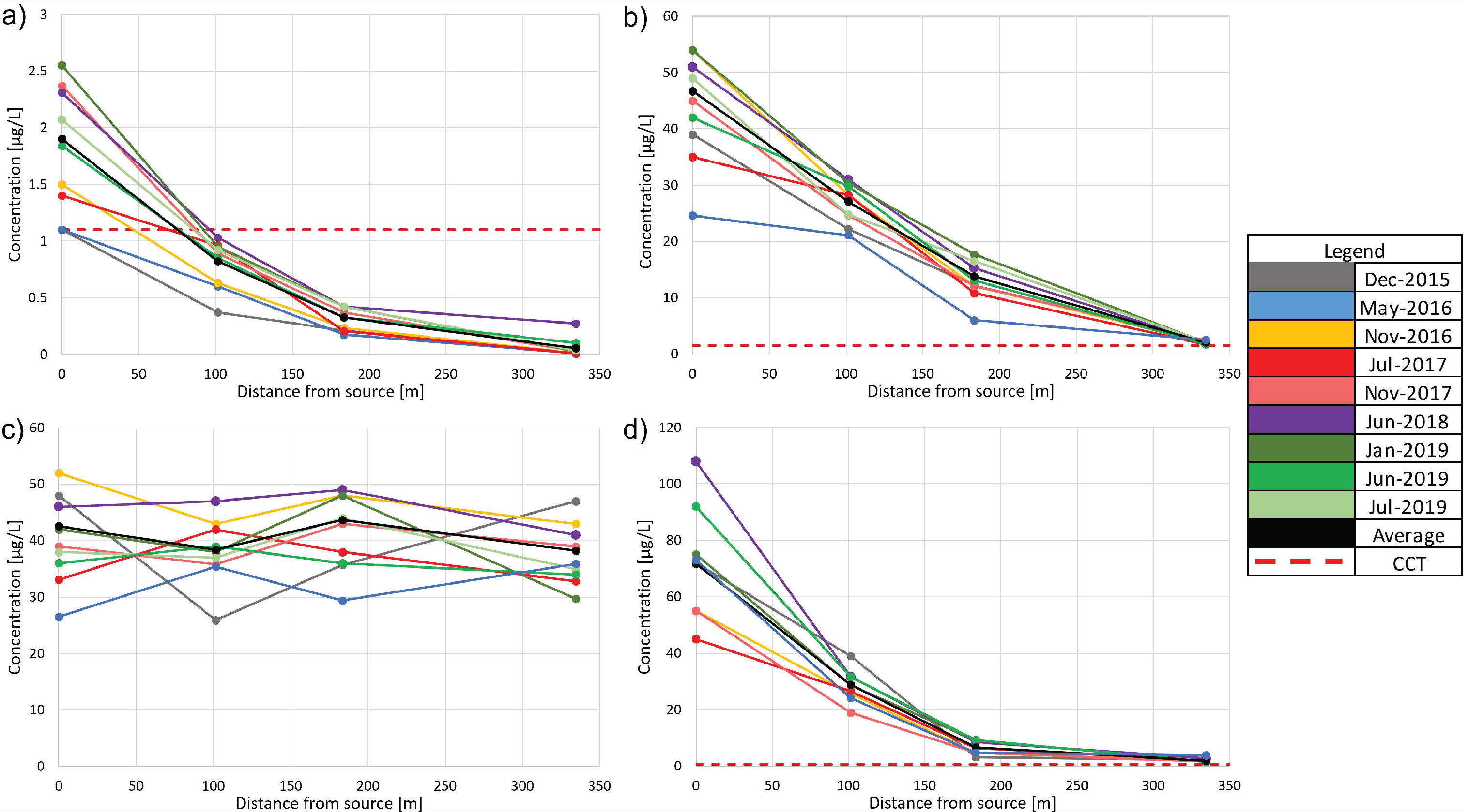
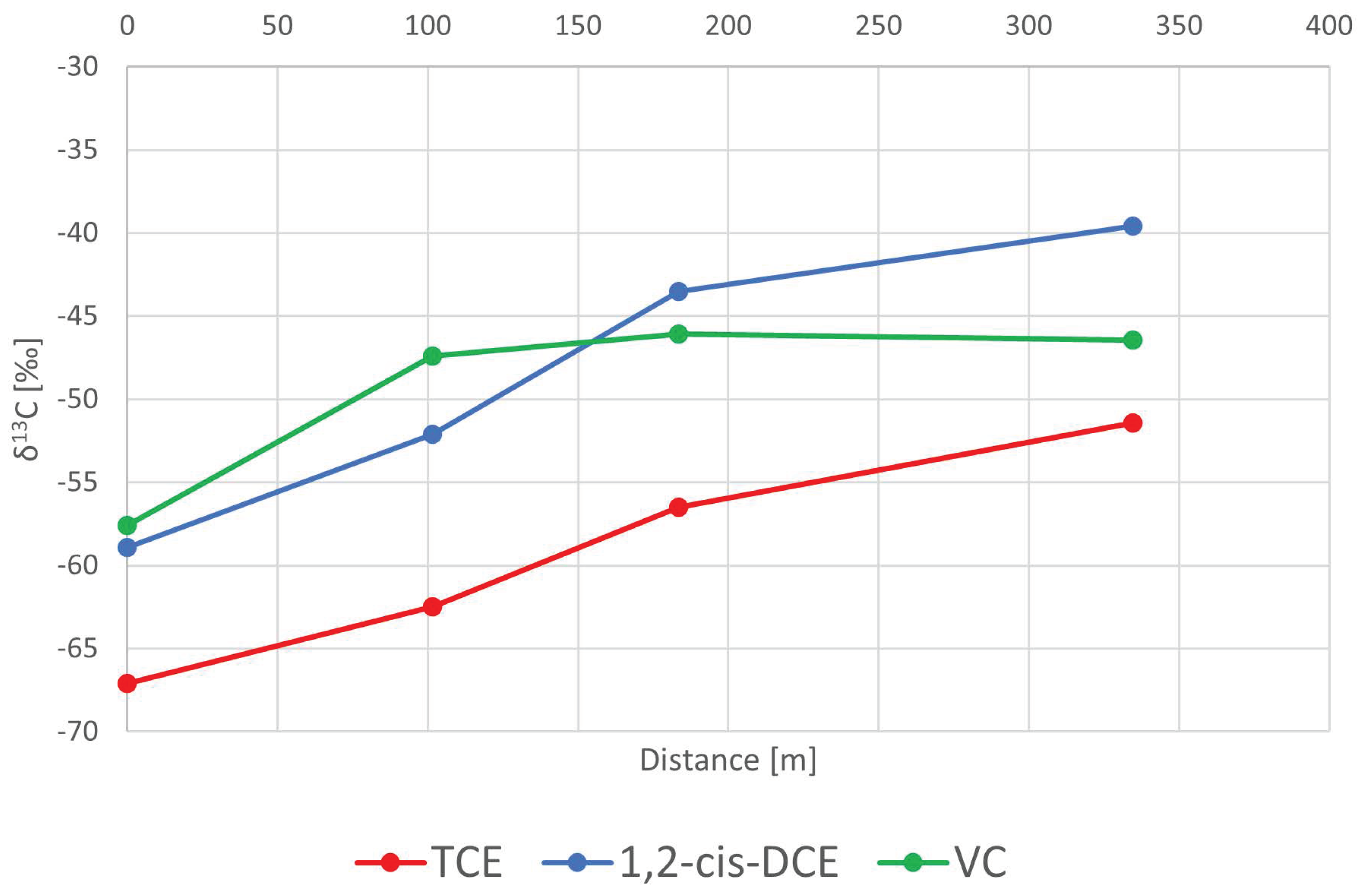
2.2.2. Analysis of Historical Concentrations and Isotopic Composition

The database of the historical concentrations available for the site spans from 2001 to 2019, however, for the purposes of the present work only the analytic campaigns performed from 2015 were used (Figure 2), due to differences in the analytical methods and the presence of many missing values in the database of the 4 monitoring wells for the previous years. The concentration analysis showed that the wells along the plume path are p9, p10, p11, p12, PN1, PN2 and PN3, however the last three points were excluded from the analyses, since only one analytical campaign and no isotopic composition data were available. Furthermore, the position of well p10 can influence the detected concentration, because it is not perfectly positioned along the hypothesized plume center line.

Since no contamination was detected in the wells upstream of p9 and the concentrations in this well were similar to the one measured in well PN1, it was assumed that p9 may likely represents the source concentrations.

The presence of PCE, TCE, 1,2-cis-DCE, VC, and ethene indicates that reductive dechlorination is active in the area. The concentrations of all components, except for the 1,2-cis-DCE, tend to decrease with distance from the source, whereas they remain almost constant in the different piezometers over time (except for seasonal variations or exceptional years). The almost constant values of 1,2-cis-DCE over space can be explained by a balanced production and consumption of the compound, following the reductive dechlorination degradation chain. While the concentrations of PCE are relatively low (even though in p9 it is still above the CCT equal to 1.1 µg/L), the other compounds show significant abundance. TCE and VC concentrations exceed the CCT defined by the Italian law (152/06, 1.5 µg/L and 0.5 µg/L respectively) in each piezometer, while 1,2-cis-DCE is always below the threshold value (152/06 sets a limit of 60 µg/L only for total 1,2-DCE).

The analyses of isotope values is very important and can support the interpretation of the concentration values. Study [69] showed strongly depleted carbon signatures and chlorine and hydrogen signatures similar to literature values of the 2 field cases; this was the proof that by means of a multi-element CSIA approach, the identification of sources and site-specific processes affecting chloroethene transformation in groundwater can be better interpreted. Concerning the measured carbon isotopic composition (shown in Figure 3), the available data is limited to one analytic survey in 2014 for TCE, 1,2-cis-DCE, and VC only (PCE shows very low concentrations). Moving away from the source, there is significant isotopic enrichment (i.e., less negative isotopic composition), indicating active biodegradation of these compounds. During biodegradations, the lighter isotope is consumed more rapidly because it is easier for bacteria to break bonds (metabolize) containing the light isotope [14]. This fractionation process is not significantly influenced by sorption or dilution [70,71,72]. There is enrichment phenomenon for TCE and 1,2-cis-DCE, whereas VC tends to maintain a constant isotopic composition downgradient of well p10, showing that the degradation stops (no more fractionation occurs). The isotopic composition for all compounds is particularly negative compared to the literature values; this specific characteristic is due to the production process that started from a local methane gas reservoir, which is characterized by very depleted levels [73,74].

Concerning the concentrations and isotopic composition analysis, some essential conclusions can be drawn. The concentration values can be assumed to be representative of a steady state condition because the values are constant over the time. Similar to concentration values, the isotopic composition can be assumed to be in steady-state conditions as initial hypothesis, missing new isotopic analyses. A clear presence of the compounds, which belong to the reductive dechlorination chain of chloroethenes, was shown indicating that this biodegradation reaction is occurring. The CSIA shows evidence of biodegradation for all the chlorinated solvents and the abundance of such compounds entails a potentially harmful situation and marks the site as “contaminated”, given that the concentration of some compounds is above the Italian CCTs.

2.2.3. Conceptual Site Model Setup

Based both on the hydrogeological setting and on the concentrations and isotopic composition analyses, a Conceptual Site Model (CSM) was developed to represent a simple but comprehensive overview of the situation, in order to show the potential contaminant’s pathways, the interfering elements and the potentially sensible receptors. The sandy gravel layer, where the groundwater flows, was assumed homogeneous since no evidence of sub-layers with different permeabilities was found during the field surveys. The source potential location was identified to be a few meters upgradient of well p9, a hypothesis confirmed by a recent additional characterization campaign that shows no contamination in the upgradient wells and soils (Figure 1, clean wells). Some wells were recently drilled close to the historical ones during this characterization procedure (PN1, PN2 and PN3) showing that the plume spreads also eastwards with generally lower concentrations, defining the plume fringe. However, these concentration data were not taken into account during the analysis, since only one measure over the time was available for such points. A leakage of chlorinated solvents from storage tanks or improper removal in the proximity of the production facilities was assumed. Due to the chemical-physical characteristics of these compounds (DNAPL), they either deeply penetrated in the aquifer causing a contaminant pool or were adsorbed on a low-permeability layer, which continuously and slowly released the pollutants in the aquifer (e.g., following a back-diffusion mechanism, such as in [68]). The CHCs move downgradient of the source in accordance with the natural groundwater flow direction along the containment wall, towards the site boundaries, showing important decreases in the concentration values. Therefore, since no active measures are employed at the site, strong natural attenuation effects are evidently active in the area enclosing the above shown piezometers. In particular, the reductive dechlorination almost completely degrades the higher chlorinated compounds into final non-harmful compounds (ethene).

2.2.4. Analytical and Numerical Model Setup

Implementing the analytical and numerical models, some hypotheses are necessary to simplify the complexity of IF-RTM and to compare the two models:

• 1D simulations, due to the simple hydrogeological setting
• homogeneous aquifer properties
• the degradation follows a 1st order kinetic with a 1:1 molar stoichiometry
• degradation rate constants and enrichment factors are set constant
• the only degradation process is the reductive dechlorination, with a simplified reaction chain, i.e., only TCE, 1,2-cis-DCE, and VC are produced and consumed
• the degradation takes action only in the dissolved phase
• the source is located in proximity to well p9 and contains TCE, 1,2-cis-DCE, and VC.

PCE was not considered because of the low concentrations. The homogeneous aquifer properties are summarized in

Table 2. Groundwater flow, sorption, and advective-dispersive transport parameters.

Parameter	Symbol	Value	Unit
Domain length	L	334	m
Total simulation time	-	50	y
Average pore water velocity	$v_r$	${10}^{-5}$	m/s
Hydraulic conductivity	$k$	$6\times {10}^{-4}$	m/s
Hydraulic gradient	$i$	0.003	-
Effective porosity	θ	0.2	-
Longitudinal dispersivity	${\alpha }_L$	10	m
Transversal and vertical dispersivity	${\alpha }_{T,V}$	0	m
Bulk density	${\rho }_{bulk}$	1.7	g/cm3
Fraction of organic carbon 1	$f_{oc}$	0.0034	-

¹ Average value of 3 soil samples taken below a depth of 3.7 m in the study area.

, while the initial estimated values of the degradation rate constants (following [75]) and enrichment factors (set as the median value calculated from the statistical analysis in Table S4, Supplementary file S1) are presented in the (Table S3, Supplementary file S1), together with the initial concentration and isotopic composition in the source (well p9). In particular, the hydraulic conductivity was derived from 11 pumping tests available for the site, whereas the effective porosity and longitudinal dispersivity was achieved using literature analyses. The initial concentration value in p9 for the different compounds was selected to be equal to the average values measured since 2015 (which is the year from which complete and consistent analytical measurements are available), while the initial isotopic composition was set equal to the only available isotopic campaign, assuming the steady-state condition hypothesis.

Furthermore, the effect of the sorption was considered. Applying Equation (7), the retardation factors were evaluated for each compound and an average value $R_{d,model}$ was calculated equal to 3.74 (see Table S4 in Supplementary file S1).

The spatial and temporal discretizations in the PHREEQC model are shown in

Table 3. Parameters selected for the PHREEQC model.

Parameter	Interpretative Model	Forecast Model	Unit
	Value
Cell number	29	150	-
Shift number 1	350	79	-
Time step length	4,444,444	4,444,444	s
Flow direction	Forward	forward	-
Boundary Conditions (BCs)	constant—flux	constant—flux	-
Cell lengths	12	12	m

¹ Shift number = number of time steps.

, while the complete code is available in the Supplementary file S4.

In the forecast model, the number of cells was varied and increased to 150, extending the domain up to 1800 m. Furthermore, the shift number was adapted in order to reach the complete cleanup time (about 11 years, when all the concentrations are below the relative CCT) and to get solutions at specific times.

In this case, the sequential dechlorination considers only TCE, 1,2-cis-DCE, and VC, therefore the PHREEQC code was adapted. The initial concentration of the light and heavy isotopes was calculated for each compound following Equations (2)–(4), starting from the isotopic composition measured in p9 (Figure 3).

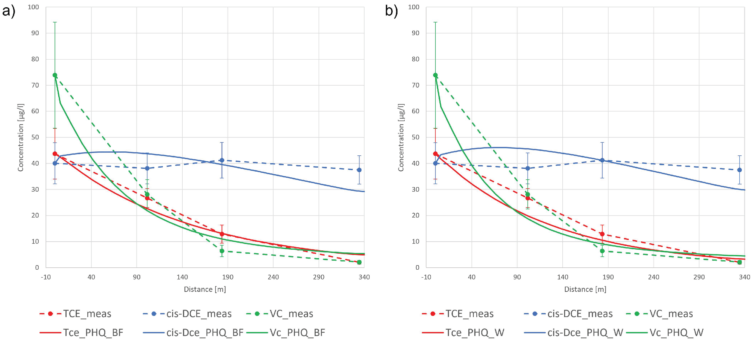
2.2.5. Model Calibration

The aim of the calibration process is to minimize an objective function that represents a least-squares estimate of the fit between field observations and computed values [76].

In the present study, in order to achieve a good agreement between the computed and the observed values, the model degradation rate constants and enrichment factors were simultaneously calibrated through the optimization code PEST [77], relying on the observed concentrations and isotopic composition data. The assisted calibration is a technique that allows the calibration to be sped up by widely spanning the parameters variability through the minimization of the error variance; it is often applied in optimization procedures of complex flow models, transport models and RTMs [59,78,79,80,81,82,83,84]. The upper and lower calibration bounds for the degradation rate constants were set as the minimum and the maximum values for each compound indicated by [85], respectively. Boundary values for enrichment factors were set by applying the same logic: a statistical analysis concerning enrichment factors data coming from the BIOCHLOR-ISO database [51] and the website www.isodetect.de (accessed on 18 November 2020) (see Figure S2 and Table S5 in Supplementary file S1 and the database presented in Supplementary file S3) was carried out.

The parameters are subsequently updated by the code in order to minimize an objective function PHI (Equation (10)), defined as the sum of the squared residuals between computed and observed values:

$$\mathrm{PHI}={\displaystyle \sum }_i{\left(y_i-y_{obs}\right)}^2$$

(10)

where $y_i$ and $y_{obs}$ are the concentration or isotope ratio computed and observed values, respectively. The observations were divided in two groups, one for concentration and one related to the isotope ratios, in order to quantify the error associated to each group. The resulting overall objective function value (PHI) was 248.28, with a contribution of the concentrations PHI_conc = 195.83 and of the isotope ratios of PHI_iso = 52.45.

A second calibration was performed weighting the observation relative to well p10, considering that the position of this well is not strictly along the plume center line, and thus the detected values may be biased. The initial parameter values were set equal to the first calibration results. Selecting a weighting factor of 0.25 for these observations, the calibration led to an overall PHI value of 135.58, with a contribution of the concentrations PHI_conc = 85.92 and of the isotope ratios of PHI_iso = 49.66.

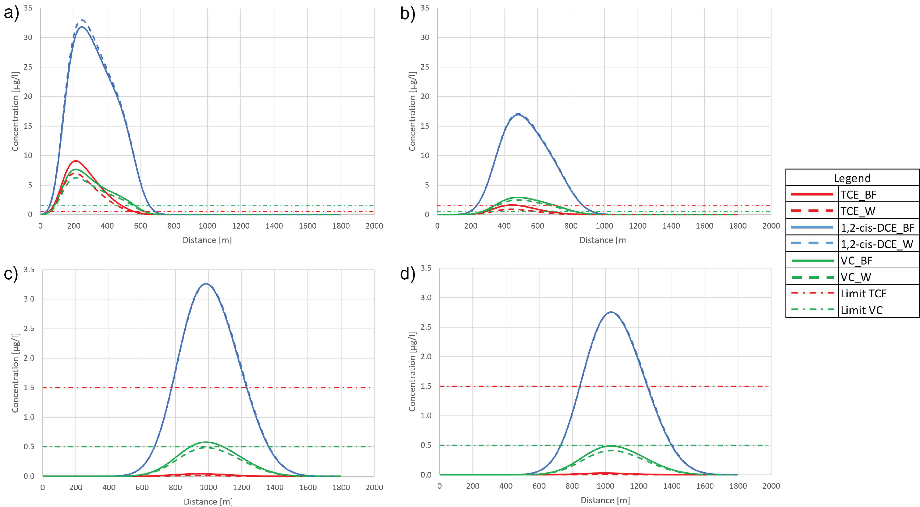
2.2.6. Predictive Model

The calibrated model was then used to forecast the remediation time frame according to the hypothesis of complete source removal by active methods. The model was divided by three Stress Periods (SPs,

Table 4. Predictive model SPs definition.

Stress Period	Period	Duration (Days)	Initial Conditions
SP1	Pre-source removal	204	Steady-state concentrations
SP2	During source removal	204	Half of the steady-state concentrations
SP3	Post-source removal	variable 1	Null

¹ variable = variable duration, adapted to search for the remediation time frame.

), representing the pre-source removal situation (204 days); the source removal work period (204 days), where the concentrations were assumed half of the initial ones; and the post-source removal period, where the source concentration was set to be null. Varying the last period length (SP3), the remediation time frame was selected to be as long as it was necessary to reach compound concentrations below the CCT set by the Italian law.

The PHREEQC code was adapted both assuming a linear trend of the concentrations among the wells and introducing the corresponding concentration as initial concentration in each cell of the model (a total of 29 initial concentrations, one for each model cell). This allowed the initial conditions of SP1 for the presence of a well-developed and stable plume (June 2019) to be correctly reproduced. Moreover, the model domain was extended up to 2000 m from the source (the aquifer extends more than 2 km) in order to check the time frame for which concentrations were below the CCT in the aquifer.

3. Results

The PHREEQC code was initially compared to BIOCHLOR-ISO for two synthetic cases to validate the code with an analytical solution. In the first case, concentrations and isotopic composition were calculated along a contaminant plume downstream of the source consisting of chlorinated ethenes (PCE, TCE, 1,2-cis-DCE, and VC). Then, in the second case, the two models were compared by considering sorption effects through Breakthrough (BT) curves 200 m downstream of the source, maintaining the same source mix as in case 1. The two models were then used to implement an interpretative model of a real contaminated site, modeling concentrations, isotopic compositions, and sorption effects. Finally, the validated PHREEQC model was used for a predictive analysis in a Natural Attenuation scenario to forecast the remediation time frame.

3.1. Synthetic Case

3.1.1. Case 1

Concerning the synthetic case 1, Figure 4a compares the concentration values in space along the plume center line while Figure 4b shows the isotopic composition calculated by the two models.

The simulated concentrations over the time and space achieved through PHREEQC agree almost perfectly to those achieved by BIOCHLOR-ISO, as well as the isotopic composition calculated by the two models. The computed RMSE between the two results is 0.0062 mM for the concentrations and 0.17‰ for the isotopic composition. These results show good agreement, therefore PHREEQC can be considered a suitable and reliable code for RTM simulations.

3.1.2. Case 2

Concerning the synthetic case n.2, Figure 5 shows the results of the comparison between the BT curves computed by PHREEQC and BIOCHLOR-ISO version 2016 at 200 m downgradient of the source. Figure 5a shows the BT curves without implementing the sorption effects, while Figure 5b considers sorption mechanisms through the implementation of a retardation factor $R_d=$ 2.14.

Also, in this case, the model results show good agreement with an RMSE equal to 0.01 mM in both cases.

3.2. Real Case

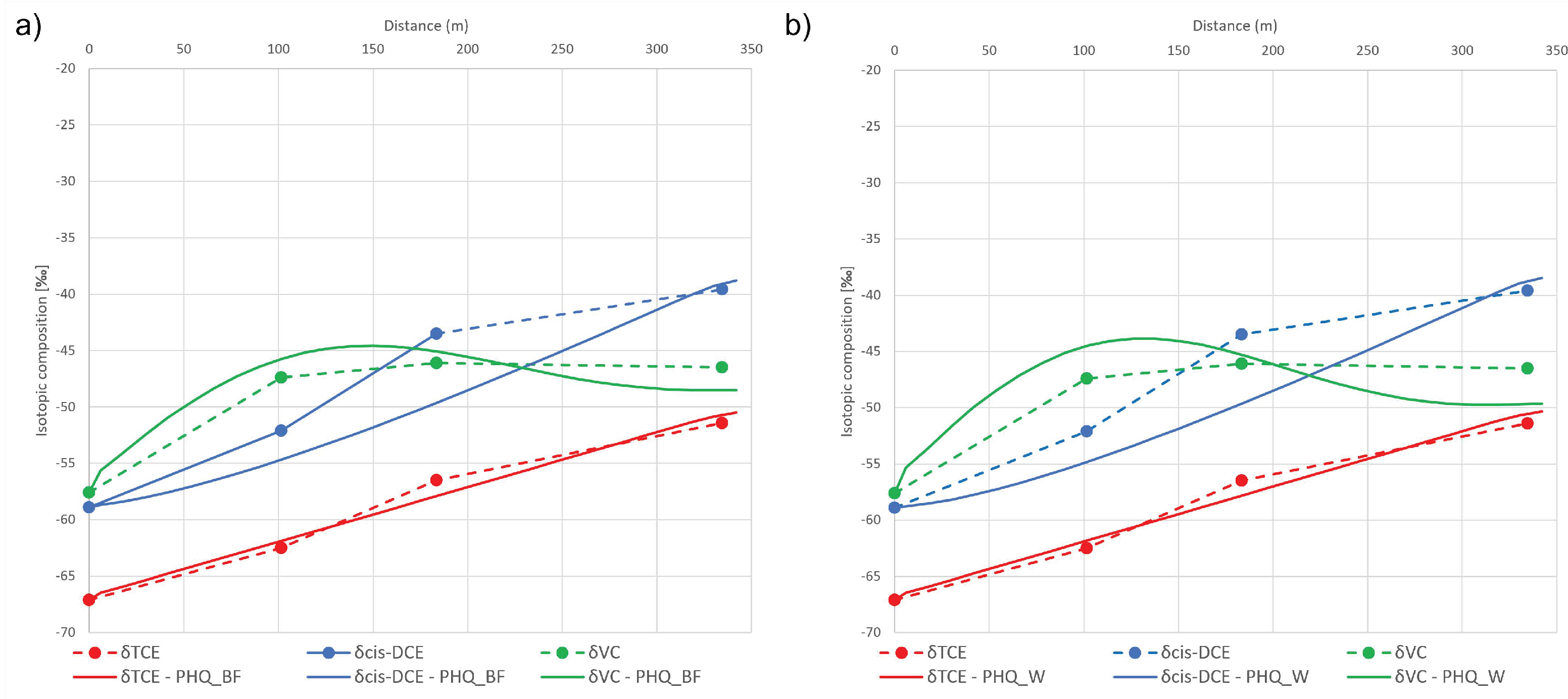
3.2.1. Interpretative Model

The first important result applying RTM to the real case was the identification of the most reliable degradation rate constant values by means of a calibration process. Both the trial-and-error and the assisted calibration (PEST) approaches can be used, but to reduce the time expenditure, the second approach was chosen. The calibration process is a crucial and necessary step to properly set the model for any following predictive simulations. Figure 6 shows the concentrations resulting from the model after the calibration process of the degradation rate constants in the Best Fit (BF) parameters case and the weighted (W) case. The results of BIOCHLOR-ISO and PHREEQC agreed well also in the real case (the comparison in the Best Fit case is shown in Supplementary file S1, Figure S1). The associate calibrated values and corresponding RMSE before and after the calibrations are shown in

Table 5. Degradation rate constants and RMSE values for the concentrations. For the degradation rate constants, two different values are presented: the actual degradation rate constant values (λ) on the left and the degradation rate constant considering sorption effects on the right (λ/R).

Compound	Pre-Calibration			Best Fit			Weighted
	λ [1/y]	λ/R [1/y]	RMSE [µg/L]	λ [1/y]	λ/R [1/y]	RMSE [µg/L]	λ [1/y]	λ/R [1/y]	RMSE [µg/L]
TCE	3.20	0.86	5.61	2.22	0.59	2.53	2.64	0.71	1.45
1,2-cis-DCE	0.045	0.012	25.01	1.040	0.28	4.52	1.02	0.27	3.32
VC	3.85	1.03	3.11	4.80	1.28	4.01	5.43	1.45	2.58

.

The results of the calibration of the enrichment factors are shown in Figure 7, while the calibrated values and the corresponding RMSE are shown in

Table 6. Enrichment factors and RMSE values relative to the isotope composition.

Compound	Pre-Calibration		Best Fit		Weighted
	ε [‰]	RMSE [‰]	ε [‰]	RMSE [‰]	ε [‰]	RMSE [‰]
TCE	−22.9	28.88	−8.2	1.32	−7.1	1.35
1,2-cis-DCE	−30.5	16.89	−30.5	3.50	−30.5	3.26
VC	−31.2	43.34	−15.9	0.66	−16.0	1.17

.

The calibration process satisfactorily adapted the parameters to the field-measured concentrations: the comparison between the simulated curves and the measured values agrees quite well and an improvement related to the pre-calibration simulations is clear. However, the VC isotopic values computed by PHREEQC show a first enrichment of the isotopic composition but, after p10, the curve decreases showing more depleted values. This behavior can be explained as an effect of VC production and consumption balance. Around p9, the VC shows higher concentrations that rapidly decrease towards p12, while the 1,2-cis-DCE shows almost constant values (around 40 µg/L) throughout the whole domain. Therefore, a huge amount of VC is degraded in the first part of the domain, resulting in an enrichment of the isotopic composition. However, downgradient of p10, the production of depleted VC by the 1,2-cis-DCE degradation results in an overall decrease of ¹³C concentration and, therefore, in more depleted values, effect that is enhanced by the higher enrichment factor of 1,2-cis-DCE.

The PHREEQC results were also compared with the analytical solution of BIOCHLOR-ISO achieving good agreements; therefore, this is an additional validation of the numerical code for a real case.

The calibrated parameters were then compared with literature values to verify whether the values were acceptable in comparison with the existing field measurements. The degradation rate constants were compared with the values reported by [85], which performed a statistical analysis on 185 field or laboratory measured degradation rate constant data. All the calibrated parameters are included in the box-plot within the 25° and 75° percentile and are quite close to the median values (except for the TCE value, which is closer to the 75th percentile). Therefore, the calibration process can be considered consistent with the literature values.

In order to compare the calibrated enrichment factors with literature values, a statistical analysis was performed relying on 179 enrichment factors available in the literature (See Table S5 in Supplementary file S1), mainly from microcosm studies, both in aerobic and anaerobic conditions. The comparison is shown in Figure 8.

The calibrated TCE enrichment factor is acceptable and comparable with anaerobic degradation. The 1,2-cis-DCE calibrated enrichment factor falls on the lower whisker of the anaerobic boxplot. This value seems to be extreme but is nonetheless acceptable. Moreover, the modeled isotopic composition of 1,2-cis-DCE shows the biggest error among the different compounds, as previously discussed, indicating complex degradation. Finally, the VC enrichment factor value falls between the boxes relative to the aerobic and anaerobic conditions, indicating that the degradation conditions can be mixed.

3.2.2. Predictive Model

Once the RTM parameters were calibrated, according to the detected concentrations and isotope signatures, PHREEQC was applied to predict the natural attenuation effects on chloroethenes following a hypothetical source removal. In Figure 9, the results for three different time frames show the concentrations change after the source remediation, comparing the achieved solution using the parameters calibrated for the Best Fit case (BF) and the weighted case (W).

The graphs show an important reduction in the concentrations along the plume line, following the contamination source removal: 500 m downstream of the source, after just 5 years TCE and VC concentrations are less than 3 µg/L and just above the CCT. A complete site remediation is predicted to be achieved after 3876 days (10.6 years) in the weighted calibration parameters case (W), whereas after 4080 days (11.2 years) in the Best Fit (BF) parameters case. Conversely, considering a non-degradative model, the concentrations decrease less rapidly with a remediation time greater than 30 years (see Figure S2 in Supplementary file S1).

4. Discussion

The reported case study shows how the design of the remediation actions needs to assess the presence of Natural Attenuation processes and include them in the prediction modeling. The aim of the paper is to show that even simple 1D models can help to assess the field conditions and can be used only as a preliminary feasibility tool for Natural Attenuation remediation procedures. Additionally, 1D models can be useful for simple hydrogeological settings, such as the one discussed here. Nevertheless, it is important to follow a series of steps to achieve reliable predictions. After the site hydrogeological characterization, the analysis of monitored concentration over space and time, as well as the identification of the contaminants’ attenuation and degradation products, represents the first essential step. Moreover, CSIA can provide an added value in confirming the presence of degradation processes, excluding that the concentration reduction is given by mechanical dispersion, dilution, sorption or volatilization. Monitoring the isotopes in water samples is not a common or widespread technique but is often considered an added value. Indeed, once this information is available, it can be used to support the remediation design starting from the modeling phase.

In the real case presented herein, the site characterization indicates the presence of chlorinated ethenes, mainly TCE, 1,2-cis-DCE, and VC, whose source is assumed to be located upgradient of well p9. The supporting CSIA analyses on C isotopes and the concentration trends clearly indicate the occurrence of a steady-state plume that is undergoing biodegradation due to reductive dechlorination processes. The hydrogeological setting is simple because the aquifer is included into a uniform sandy gravels layer, which rests on a silty clay layer at the bottom. The silty clay layer could have produced the back-diffusion phenomenon over time and from concentration and isotopes analyses, the situation can be approximated as in steady-state condition. Therefore, the hydrogeological and contamination background discussed makes the site suitable for a combined remediation approach between an active source removal method and MNA to clean up the residual concentrations.

Then, a reliable numerical code is necessary for the modelling phase. The present study confirms that PHREEQC is a multidisciplinary code that can be adapted to reproduce the Natural Attenuation processes in aquifers. During the design phase, this code is indeed a useful tool to support both the remediation techniques based on biodegradation and the best possible alternative. The modeling phase requires a proper calibration of the transport parameters. In the present case, the adopted simultaneous calibration (carried out using PEST) of the degradation rate constant and isotope enrichment factor represents an added value because it considers the relative effect that one parameter group has on the other. Using the assisted calibration instead of a trial-and-error approach allows easy determination of an optimized solution and is a method seldomly used in IF-RTMs calibration.

The calibrated degradation rate constant values were compared with the statistical analysis performed by [85], with the selected values within the 25th and 75th percentiles of the population and comparable to anaerobic degradation. Moreover, the calibrated enrichment factors were compared with the statistics calculated on the database presented as Supplementary file S3. The TCE values were coherent with anaerobic degradation, while the ones for VC and 1,2-cis-DCE show values that may involve mixed conditions. In particular, the 1,2-cis-DCE enrichment factor was close to the lower extreme boundary of the aerobic conditions and outside the lower whisker of the anaerobic values. This issue cannot be neglected since two factors could affect the results. First, only one isotopic survey is available for the site (in 2014) and second, the enrichment factors database includes many values derived from both laboratory and field studies, which are strongly dependent on specific site conditions. Therefore, no values can be excluded, even if they fall outside the whisker. To properly design an executive remediation project, a new isotopic survey and new microcosm experiments should be executed in order to further constrain the model parameter ranges.

A potential limitation of this model is the simple 1D simulation, which could neglect the transversal dispersivity, which in some cases determines a reduction in the mass flowing along the plume center line. This influences the values of the targets used during the calibration process and, consequently, PEST adapts the degradation rate constant values, adjusting them to represent the transversal dilution effect. This issue affects the absolute values of the degradation rate constants but not the solution reliability, since the concentration reduction due to transversal dispersion is included. However, the 1D approach allows easy representation of the reactive transport occurring at the site, owing to the homogeneous hydrogeological setting, and contemporarily interprets and represents the simple Natural Attenuation processes occurring at the site quite well. For a more complex hydrogeological case, the model can be further improved through representation of 2D conditions by introducing trace tests to better estimate the dispersivity, by planning more isotopic campaigns and extending the CSIA to chlorine atoms using a dual-isotope approach, or by more thoroughly investigating the biodegradation of 1,2-cis-DCE and VC.

If MNA is selected as the remediation strategy, in general and for more complex cases, it should be accompanied by a structured monitoring network and planning. For example, in order to better characterize the site, new wells can be drilled downgradient of p12 in order to check that no contaminants exit from the site boundary and a backup system can be provided (e.g., Pump-and-treat P&T), in case MNA does not work as expected. However, the model shows that in simple geological contexts MNA can be a preferable technique to active strategies, such as P&T, as it is both an effective and a low-cost option.

5. Conclusions

This paper evaluates the applicability of MNA as possible a remediation strategy for a site contaminated by chlorinated solvents by means of a 1D numerical model in a field case where hydrogeological conditions are simple. First, the analytical model BIOCHLOR-ISO and the numerical code PHREEQC were compared assuming two different conditions, i.e., considering an IF-RTM and the sorption effects. The comparison showed good agreement in each case, for both the concentrations and the isotopic composition; therefore, PHREEQC is a reliable code that can be used for IF-RTMs and is more appropriate than BIOCHLOR-ISO because it is able to simulate transient conditions. Moreover, this PHREEQC property allows the coupling with common 2D or 3D hydrogeological codes in order to carry out more detailed results.

Subsequently, a CSM of a chlorinated solvents-contaminated site located in southern Italy was developed and converted into a 1D steady-state IF-RTM. The degradation rate constants were initially estimated by means of the method presented by [86] and the enrichment factors were selected carrying out a statistical analysis on 179 values collected from literature research. The flow and transport parameter values were derived from field data. Then, the numerical models were calibrated by using the optimization code PEST, calibrating the degradation rate constants and the enrichment factors simultaneously.

The calibrated model was finally used to forecast the remediation time frame. Assuming the hypothesis of complete source removal, the remediation time frame was determined to be about 11 years, making the site suitable for MNA application. The computed remediation time is reasonably short and a MNA procedure can be easily applied in this case because of the implicit hypothesis and of the simplicity of the site (hydrogeological setting, few monitoring wells, etc.). The solution was compared with a non-degradative case, showing that the remediation time frame without degradation would have been much longer than 30 years. This is further evidence of how RTM can provide an estimate of remediation times with or without degradation processes, in order to help engineers or agencies to clean up polluted sites.

In conclusion, even if MNA is not yet diffused as a common remediation strategy in Italy, this application study shows the potential and value, which can be relevant for similar industrial sites. IF allows researchers to confirm that degradation (bond-braking reactions), not only dispersion, dilution and sorption are active; therefore, this strongly supports MNA. This study provides a stepwise methodology that can be applied to preliminary evaluate the feasibility of the MNA approach application. For this case, the model is also able to provide an estimation of the remediation time frame that can be helpful to site owners and Public Authorities in the process of selecting a suitable remediation strategy that is both effective in reasonable time frames and as low-cost as possible.

References

1. Doherty, R.E. A History of the Production and Use of Carbon Tetrachloride, Tetrachloroethylene, Trichloroethylene and 1,1,1-Trichloroethane in the United States: Part 2—Trichloroethylene and 1,1,1-Trichloroethane. Environ. Forensics 2000, 1, 83–93. [Google Scholar] [CrossRef]
2. Doherty, R.E. A History of the Production and Use of Carbon Tetrachloride, Tetrachloroethylene, Trichloroethylene and 1,1,1-Trichloroethane in the United States: Part 1—Historical Background; Carbon Tetrachloride and Tetrachloroethylene. Environ. Forensics 2000, 1, 69–81. [Google Scholar] [CrossRef]
3. Mccarty, P.L. Groundwater Contamination by Chlorinated Solvents: History, Remediation Technologies and Strategies; Springer: Berlin/Heidelberg, Germany, 2010; pp. 1–28. [Google Scholar]
4. Stroo, H.F.; Ward, C.H. In Situ Remediation of Chlorinated Solvent Plumes; Springer: Berlin/Heidelberg, Germany, 2010; ISBN 1441914013. [Google Scholar]
5. Wiedemeier, T.; Swanson, M.; Moutoux, D.; Gordon, E.; Wilson, J.; Wilson, B.; Kampbell, D.; Haas, P.; Miller, R.; Hansen, J.; et al. Technical Protocol for Evaluating Natural Attenuation of Chlorinated Solvents in Ground Water; United States Environmental Protection Agency: Washington, DC, USA, 1998.
6. Zanini, A.; Ghirardi, M.; Emiliani, R. A multidisciplinary approach to evaluate the effectiveness of natural attenuation at a contaminated site. Hydrology 2021, 8, 101. [Google Scholar] [CrossRef]
7. Maymó-Gatell, X.; Chien, Y.T.; Gossett, J.M.; Zinder, S.H. Isolation of a bacterium that reductively dechlorinates tetrachloroethene to ethene. Science 1997, 276, 1568–1571. [Google Scholar] [CrossRef]
8. He, J.; Ritalahti, K.M.; Aiello, M.R.; Löffler, F.E. Complete detoxification of vinyl chloride by an anaerobic enrichment culture and identification of the reductively dechlorinating population as a Dehalococcoides species. Appl. Environ. Microbiol. 2003, 69, 996–1003. [Google Scholar] [CrossRef] [Green Version]
9. Němeček, J.; Marková, K.; Špánek, R.; Antoš, V.; Kozubek, P.; Lhotský, O.; Černík, M. Hydrochemical Conditions for Aerobic/Anaerobic Biodegradation of Chlorinated Ethenes—A Multi-Site Assessment. Water 2020, 12, 322. [Google Scholar] [CrossRef] [Green Version]
10. Dempster, H.S.; Lollar, B.S.; Feenstra, S. Tracing organic contaminants in groundwater: A new methodology using compound-specific isotopic analysis. Environ. Sci. Technol. 1998, 31, 3193–3197. [Google Scholar] [CrossRef]
11. Hunkeler, D.; Aravena, R. Determination of compound-specific carbon isotope ratios of chlorinated methanes, ethanes, and ethenes in aqueous samples. Environ. Sci. Technol. 2000, 34, 2839–2844. [Google Scholar] [CrossRef] [Green Version]
12. Hunkeler, D.; Aravena, R.; Butler, B.J. Monitoring microbial dechlorination of tetrachloroethene (PCE) in groundwater using compound-specific stable carbon isotope ratios: Microcosm and field studies. Environ. Sci. Technol. 1999, 33, 2733–2738. [Google Scholar] [CrossRef] [Green Version]
13. Hunkeler, D.; Aravena, R.; Parker, B.L.; Cherry, J.A.; Diao, X. Monitoring oxidation of chlorinated ethenes by permanganate in groundwater using stable isotopes: Laboratory and field studies. Environ. Sci. Technol. 2003, 37, 798–804. [Google Scholar] [CrossRef] [Green Version]
14. Aelion, C.M.; Höhener, P.; Hunkeler, D.; Aravena, R. Environmental Isotopes in Biodegradation and Bioremediation; CRC Press: Boca Raton, FL, USA, 2009; ISBN 9781420012613. [Google Scholar]
15. Looney, B.; Heitkamp, M.M.; Wein, G.; Bagwell, C.C.; Vangelas, K.K.; Adams, K.K.-M.; Gilmore, T.; Cutshall, N.; Major, D.; Truex, M.; et al. Characterization and Monitoring of Natural Attenuation of Chlorinated Solvents in Groundwater: A Systems Approach; Pubinfo: Aiken, SC, USA, 2006. [Google Scholar]
16. Declercq, I.; Cappuyns, V.; Duclos, Y. Monitored natural attenuation (MNA) of contaminated soils: State of the art in Europe—A critical evaluation. Sci. Total Environ. 2012, 426, 393–405. [Google Scholar] [CrossRef]
17. Rügner, H.; Finkel, M.; Kaschl, A.; Bittens, M. Application of monitored natural attenuation in contaminated land management-A review and recommended approach for Europe. Environ. Sci. Policy 2006, 9, 568–576. [Google Scholar] [CrossRef]
18. Clement, T.P.; Truex, M.J.; Lee, P. A case study for demonstrating the application of U.S. EPA’s monitored natural attenuation screening protocol at a hazardous waste site. J. Contam. Hydrol. 2002, 59, 133–162. [Google Scholar] [CrossRef]
19. Aziz, C.E.; Newell, C.J.; Gonzales, J.R.; Haas, P.; Clement, T.P.; Sun, Y.; Jewett, D.G. BIOCHLOR Natural Attenuation Decision Support System; United States Environmental Protection Agency: Washington, DC, USA, 2000.
20. Colombani, N.; Gargini, A.; Mastrocicco, M. The use of monitored natural attenuation as a cost-effetive technique for groundwater restoration: The NIT site (ITALY). In Proceedings of the 1st International Workshop on Aquifer Vulnerability and Risk, Mexico City, Mexico, 28–30 May 2003. [Google Scholar]
21. McGuire, T.M.; Newell, C.J.; Looney, B.B.; Vangelas, K.M. Historical and Retrospective Survey of Monitored Natural Attenuation: A Line of Inquiry Supporting Monitored Natural Attenuation and Enhanced Passive Remediation of Chlorinated Solvents; Savannah River Site, Funding Organisation, US Department of Energy: Washington, DC, USA, 2003.
22. Newell, C.J.; Cowie, I.; McGuire, T.M.; McNab, W.W. Multiyear Temporal Changes in Chlorinated Solvent Concentrations at 23 Monitored Natural Attenuation Sites. J. Environ. Eng. 2006, 132, 653–663. [Google Scholar] [CrossRef] [Green Version]
23. Puigserver, D.; Herrero, J.; Parker, B.L.; Carmona, J.M. Natural attenuation of pools and plumes of carbon tetrachloride and chloroform in the transition zone to bottom aquitards and the microorganisms involved in their degradation. Sci. Total Environ. 2020, 712, 135679. [Google Scholar] [CrossRef]
24. Zhang, X.; Zhu, X.; Chen, R.; Deng, S.; Yu, R.; Long, T. Assessment of Biodegradation in Natural Attenuation Process of Chlorinated Hydrocarbons Contaminated Site: An Anaerobic Microcosm Study. Soil Sediment Contam. 2020, 29, 165–179. [Google Scholar] [CrossRef]
25. Ferrey, M.F.M.; Wilson, J.T. Complete Natural Attenuation of PCE and TCE without Vinyl Chloride and Ethene Accumulation. Available online: https://www.researchgate.net/publication/259366445_Complete_Natural_Attenuation_of_PCE_and_TCE_without_Vinyl_Chloride_and_Ethene_Accumulation (accessed on 15 September 2020).
26. Kawabe, Y.; Komai, T. A Case Study of Natural Attenuation of Chlorinated Solvents Under Unstable Groundwater Conditions in Takahata, Japan. Bull. Environ. Contam. Toxicol. 2019, 102, 280–286. [Google Scholar] [CrossRef]
27. Schiefler, A.A.; Tobler, D.J.; Overheu, N.D.; Tuxen, N. Extent of natural attenuation of chlorinated ethenes at a contaminated site in Denmark. Energy Procedia 2018, 146, 188–193. [Google Scholar] [CrossRef]
28. Kao, C.M.; Wang, Y.S. Field investigation of the natural attenuation and intrinsic biodegradation rates at an underground storage tank site. Environ. Geol. 2001, 40, 622–631. [Google Scholar] [CrossRef]
29. Kao, C.M.; Huang, W.Y.; Chang, L.J.; Chen, T.Y.; Chien, H.Y.; Hou, F. Application of monitored natural attenuation to remediate a petroleum-hydrocarbon spill site. Water Sci. Technol. 2006, 53, 321–328. [Google Scholar] [CrossRef] [PubMed]
30. Neuhauser, E.F.; Ripp, J.A.; Azzolina, N.A.; Madsen, E.L.; Mauro, D.M.; Taylor, T. Monitored Natural Attenuation of Manufactured Gas Plant Tar Mono- and Polycyclic Aromatic Hydrocarbons in Ground Water: A 14-Year Field Study. Ground Water Monit. Remediat. 2009, 29, 66–76. [Google Scholar] [CrossRef]
31. Brown, R.A.; Wilson, J.T.; Ferrey, M. Monitored natural attenuation forum: The case for abiotic MNA. Remediat. J. 2007, 17, 127–137. [Google Scholar] [CrossRef]
32. Steefel, C.I.; Appelo, C.A.J.; Arora, B.; Jacques, D.; Kalbacher, T.; Kolditz, O.; Lagneau, V.; Lichtner, P.C.; Mayer, K.U.; Meeussen, J.C.L.; et al. Reactive transport codes for subsurface environmental simulation. Comput. Geosci. 2015, 19, 445–478. [Google Scholar] [CrossRef] [Green Version]
33. Cheng, Y.; Arora, B.; Şengör, S.S.; Druhan, J.L.; Wanner, C.; van Breukelen, B.M.; Steefel, C.I. Microbially mediated kinetic sulfur isotope fractionation: Reactive transport modeling benchmark. Comput. Geosci. 2020, 25, 1–13. [Google Scholar] [CrossRef]
34. Younes, A.; Fahs, M.; Ackerer, P. Modeling of Flow and Transport in Saturated and Unsaturated Porous Media. Water 2021, 13, 1088. [Google Scholar] [CrossRef]
35. Xu, T.; Ye, Y.; Zhang, Y.; Xie, Y. Recent advances in experimental studies of steady-state dilution and reactive mixing in saturated porous media. Water 2018, 11, 3. [Google Scholar] [CrossRef] [Green Version]
36. Newell, C.J.; Mcleod, R.K.; Gonzales, J.R.; Wilson, J.T. BIOSCREEN Natural Attenuation Decision Support System; U.S. Environmental Protection Agency: Washington, DC, USA, 1996.
37. Parkhurst, D.L.; Appelo, C.A.J. User’s Guide to PHREEQC (Version 2)—A Computer Program for Speciation, Batch-Reaction, One-Dimensional Transport, And Inverse Geochemical Calculations; U.S. Geological Survey: Denver, CO, USA, 1999.
38. Prommer, H.; Davis, G.B.; Barry, D.A. PHT3D—A Three-Dimensional Biogeochemical Transport Model for Modelling Natural and Enhanced Remediation; Centre for Groundwater Studies, CSIRO: Canberra, Australia, 1999; pp. 21–25. [Google Scholar]
39. Prommer, H.; Barry, D.A.; Chiang, W.H.; Zheng, C. PHT3D-A MODFLOW/MTBDMS-based reactive multi ‘component transport model. Groundwater 2001, 41, 477–483. [Google Scholar]
40. Prommer, H.; Barry, D.A.; Zheng, C. MODFLOW/MT3DMS-based reactive multicomponent transport modeling. Ground Water 2003, 41, 247–257. [Google Scholar] [CrossRef]
41. Appelo, C.A.J.; Rolle, M. PHT3D: A reactive multicomponent transport model for saturated porous media. Ground Water 2010, 48, 627–632. [Google Scholar] [CrossRef]
42. Zheng, C.; Wang, P. MT3DMS: A Modular Three-Dimensional Multispeces Transport Model for Simulation of Advection, Dispersion, and Chemical Reactions of Contaminants in Groundwater Systems; Technical Report; Waterways Experiment Station, US Army Corps of Engineers: Washington, DC, USA, 1999. [Google Scholar]
43. Harbaugh, A.W. MODFLOW-2005, The U.S. Geological Survey Modular Ground-Water Model-the Ground-Water Flow Process; USG: Reston, VA, USA, 2005. [Google Scholar]
44. Clement, T.P.; Sun, Y.; Hooker, B.S.; Petersen, J.N. Modeling multispecies reactive transport in ground water. Gr. Water Monit. Remediat. 1998, 18, 79–92. [Google Scholar] [CrossRef]
45. Kolditz, O.; Bauer, S.; Bilke, L.; Böttcher, N.; Delfs, J.O.; Fischer, T.; Görke, U.J.; Kalbacher, T.; Kosakowski, G.; McDermott, C.I.; et al. OpenGeoSys: An open-source initiative for numerical simulation of thermo-hydro-mechanical/chemical (THM/C) processes in porous media. Environ. Earth Sci. 2012, 67, 589–599. [Google Scholar] [CrossRef]
46. Zolfaghari, R.; Chen, Z.; Shao, H.; Kuschk, P.; Kolditz, O. Multi-Component Reactive Transport Modeling of Pce Degradation at a Pilot Scale Constructed Wetland Bitterfeld; University of Illinois at Urbana-Champaign: Champaign, IL, USA, 2012; pp. 1–10. [Google Scholar]
47. Xu, T.; Sonnenthal, E.; Spycher, N.; Pruess, K. TOURGHREACT: A Simulation Program for Non-isothermal Multiphase Reactive Geochemical Transport in Variably Saturated Geologic Media. Comput. Geosci. 2004, 32, 1–203. [Google Scholar] [CrossRef] [Green Version]
48. Mayer, K.U. A Numerical Model for Multicomponent Reactive Transport in Variably Saturated Porous Media; University of Waterloo: Waterloo, ON, Canada, 1999. [Google Scholar]
49. Mayer, K.U.; Frind, E.O.; Blowes, D.W. Multicomponent reactive transport modeling in variably saturated porous media using a generalized formulation for kinetically controlled reactions. Water Resour. Res. 2002, 38, 1–21. [Google Scholar] [CrossRef]
50. Henderson, T.H.; Mayer, K.U.; Parker, B.L.; Al, T.A. Three-dimensional density-dependent flow and multicomponent reactive transport modeling of chlorinated solvent oxidation by potassium permanganate. J. Contam. Hydrol. 2009, 106, 195–211. [Google Scholar] [CrossRef] [PubMed]
51. Höhener, P.; Elsner, M.; Eisenmann, H.; Atteia, O. Improved constraints on in situ rates and on quantification of complete chloroethene degradation from stable carbon isotope mass balances in groundwater plumes. J. Contam. Hydrol. 2015, 182, 173–182. [Google Scholar] [CrossRef] [PubMed]
52. Höhener, P. Simulating stable carbon and chlorine isotope ratios in dissolved chlorinated groundwater pollutants with BIOCHLOR-ISO. J. Contam. Hydrol. 2016, 195, 52–61. [Google Scholar] [CrossRef]
53. Wexler, E.J. Analytical Solutions for One-, Two-, and Three-dimensional Solute Transport in Ground-Water Systems with Uniform Flow; USGS: Reston, VA, USA, 1992.
54. Höhener, P.; Atteia, O. Multidimensional analytical models for isotope ratios in groundwater pollutant plumes of organic contaminants undergoing different biodegradation kinetics. Adv. Water Resour. 2010, 33, 740–751. [Google Scholar] [CrossRef]
55. Höhener, P.; Atteia, O. Rayleigh equation for evolution of stable isotope ratios in contaminant decay chains. Geochim. Cosmochim. Acta 2014, 126, 70–77. [Google Scholar] [CrossRef]
56. Van Breukelen, B.M.; Hunkeler, D.; Volkering, F. Quantification of sequential chlorinated ethene degradation by use of a reactive transport model incorporating isotope fractionation. Environ. Sci. Technol. 2005, 39, 4189–4197. [Google Scholar] [CrossRef] [Green Version]
57. Van Breukelen, B.M.; Thouement, H.A.A.; Stack, P.E.; Vanderford, M.; Philp, P.; Kuder, T. Modeling 3D-CSIA data: Carbon, chlorine, and hydrogen isotope fractionation during reductive dechlorination of TCE to ethene. J. Contam. Hydrol. 2017, 204, 79–89. [Google Scholar] [CrossRef]
58. Appelo, C.; de Vet, W. Modeling in situ iron removal from groundwater with trace elements such as As. In Arsenic in Ground Water; Springer Science and Business Media LLC: Berlin/Heidelberg, Germany, 2003; pp. 381–401. [Google Scholar]
59. Appelo, C.A.J.; van der Weiden, M.J.J.; Tournassat, C.; Charlet, L. Surface complexation of ferrous iron and carbonate on ferrihydrite and the mobilization of arsenic. Environ. Sci. Technol. 2002, 36, 3096–3103. [Google Scholar] [CrossRef]
60. Sracek, O.; Bhattacharya, P.; Jacks, G.; Gustafsson, J.P.; von Brömssen, M. Behavior of arsenic and geochemical modeling of arsenic enrichment in aqueous environments. Appl. Geochem. 2004, 19, 169–180. [Google Scholar] [CrossRef]
61. Stollenwerk, K.G.; Breit, G.N.; Welch, A.H.; Yount, J.C.; Whitney, J.W.; Foster, A.L.; Uddin, M.N.; Majumder, R.K.; Ahmed, N. Arsenic attenuation by oxidized aquifer sediments in Bangladesh. Sci. Total Environ. 2007, 379, 133–150. [Google Scholar] [CrossRef]
62. Charlet, L.; Chakraborty, S.; Appelo, C.A.J.; Roman-Ross, G.; Nath, B.; Ansari, A.A.; Lanson, M.; Chatterjee, D.; Mallik, S.B. Chemodynamics of an arsenic “hotspot” in a West Bengal aquifer: A field and reactive transport modeling study. Appl. Geochem. 2007, 22, 1273–1292. [Google Scholar] [CrossRef]
63. Liu, Y.; Goor, J.; Robinson, C.E. Behaviour of soluble reactive phosphorus within field-scale bioretention systems. J. Hydrol. 2021, 601, 126597. [Google Scholar] [CrossRef]
64. Zamane, S.; Gori, D.; Höhener, P. Multistep partitioning causes significant stable carbon and hydrogen isotope effects during volatilization of toluene and propan-2-ol from unsaturated sandy aquifer sediment. Chemosphere 2020, 251, 126345. [Google Scholar] [CrossRef] [PubMed]
65. Hu, J.; Zhu, C.; Long, Y.; Yang, Q.; Zhou, S.; Wu, P.; Jiang, J.; Zhou, W.; Hu, X. Interaction analysis of hydrochemical factors and dissolved heavy metals in the karst Caohai Wetland based on PHREEQC, cooccurrence network and redundancy analyses. Sci. Total Environ. 2021, 770, 145361. [Google Scholar] [CrossRef]
66. Sprocati, R.; Masi, M.; Muniruzzaman, M.; Rolle, M. Modeling electrokinetic transport and biogeochemical reactions in porous media: A multidimensional Nernst-Planck-Poisson approach with PHREEQC coupling. Adv. Water Resour. 2019, 127, 134–147. [Google Scholar] [CrossRef]
67. Aeppli, C.; Hofstetter, T.B.; Amaral, H.I.F.; Kipfer, R.; Schwarzenbach, R.P.; Berg, M. Quantifying in situ transformation rates of chlorinated ethenes by combining compound-specific stable isotope analysis, groundwater dating, and carbon isotope mass balances. Environ. Sci. Technol. 2010, 44, 3705–3711. [Google Scholar] [CrossRef] [PubMed] [Green Version]
68. Antelmi, M.; Renoldi, F.; Alberti, L. Analytical and Numerical Methods for a Preliminary Assessment of the Remediation Time of Pump and Treat Systems. Water 2020, 12, 2850. [Google Scholar] [CrossRef]
69. Filippini, M.; Nijenhuis, I.; Kümmel, S.; Chiarini, V.; Crosta, G.; Richnow, H.H.; Gargini, A. Multi-element compound specific stable isotope analysis of chlorinated aliphatic contaminants derived from chlorinated pitches. Sci. Total Environ. 2018, 640–641, 153–162. [Google Scholar] [CrossRef]
70. Slater, G.F.; Ahad, J.M.E.; Sherwood Lollar, B.; Allen-King, R.; Sleep, B. Carbon isotope effects resulting from equilibrium sorption of dissolved VOCs. Anal. Chem. 2000, 72, 5669–5672. [Google Scholar] [CrossRef]
71. Schüth, C.; Taubald, H.; Bolaño, N.; Maciejczyk, K. Carbon and hydrogen isotope effects during sorption of organic contaminants on carbonaceous materials. J. Contam. Hydrol. 2003, 64, 269–281. [Google Scholar] [CrossRef]
72. Druhan, J.L.; Winnick, M.J. Reactive transport of stable isotopes. Elements 2019, 15, 107–110. [Google Scholar] [CrossRef]
73. Mattavelli, L.; Novelli, L. Geochemistry and habitat of natural gases in Italy. Org. Geochem. 1988, 13, 1–13. [Google Scholar] [CrossRef]
74. Nijenhuis, I.; Schmidt, M.; Pellegatti, E.; Paramatti, E.; Richnow, H.H.; Gargini, A. A stable isotope approach for source apportionment of chlorinated ethene plumes at a complex multi-contamination events urban site. J. Contam. Hydrol. 2013, 153, 92–105. [Google Scholar] [CrossRef]
75. Buscheck, T.E.; Alcantar, C.M. Regression Techniques and Analytical Solutions to Demonstrate Intrinsic Bioremediation; Battelle Press: Columbus, OH, USA, 1995; ISBN 1-57477-002-0. [Google Scholar]
76. Tonkin, M.; Doherty, J. Calibration-constrained Monte Carlo analysis of highly parameterized models using subspace techniques. Water Resour. Res. 2009, 45, 1–10. [Google Scholar] [CrossRef] [Green Version]
77. Doherty, J. PEST Model-Independent Parameter Estimation; Watermark Numerical Computing: Brisbane, Australia, 2004. [Google Scholar]
78. Van Breukelen, B.M.; Griffioen, J.; Röling, W.F.M.; van Verseveld, H.W. Reactive transport modelling of biogeochemical processes and carbon isotope geochemistry inside a landfill leachate plume. J. Contam. Hydrol. 2004, 70, 249–269. [Google Scholar] [CrossRef] [PubMed]
79. Yabusaki, S.B.; Fang, Y.; Long, P.E.; Resch, C.T.; Peacock, A.D.; Komlos, J.; Jaffe, P.R.; Morrison, S.J.; Dayvault, R.D.; White, D.C.; et al. Uranium removal from groundwater via in situ biostimulation: Field-scale modeling of transport and biological processes. J. Contam. Hydrol. 2007, 93, 216–235. [Google Scholar] [CrossRef] [PubMed]
80. Prommer, H.; Aziz, L.H.; Bolaño, N.; Taubald, H.; Schüth, C. Modelling of geochemical and isotopic changes in a column experiment for degradation of TCE by zero-valent iron. J. Contam. Hydrol. 2008, 97, 13–26. [Google Scholar] [CrossRef]
81. Antoniou, E.A.; Stuyfzand, P.J.; van Breukelen, B.M. Reactive transport modeling of an aquifer storage and recovery (ASR) pilot to assess long-term water quality improvements and potential solutions. Appl. Geochem. 2013, 35, 173–186. [Google Scholar] [CrossRef]
82. Kavousi, A.; Reimann, T.; Liedl, R.; Raeisi, E. Karst aquifer characterization by inverse application of MODFLOW-2005 CFPv2 discrete-continuum flow and transport model. J. Hydrol. 2020, 587, 124922. [Google Scholar] [CrossRef]
83. Kruisdijk, E.; van Breukelen, B.M. Reactive transport modelling of push-pull tests: A versatile approach to quantify aquifer reactivity. Appl. Geochem. 2021, 131, 104998. [Google Scholar] [CrossRef]
84. Colombo, L.; Alberti, L.; Mazzon, P.; Antelmi, M. Null-Space Monte Carlo Particle Backtracking to Identify Groundwater Tetrachloroethylene Sources. Front. Environ. Sci. 2020, 8, 142. [Google Scholar] [CrossRef]
85. Suarez, M.P.; Rifai, H.S. Biodegradation rates for fuel Hydrocarbons and Chlorinated Solvents in groundwater. Bioremediat. J. 1999, 3, 337–362. [Google Scholar] [CrossRef]
86. Buscheck, T.E.; Alcantar, C.M. Regression Techniques and Analytical Solutions to Demonstrate; International Nuclear Information System (INIS): Vienna, Austria, 1995. [Google Scholar]
Figure 1. (a) Study area, observed piezometry (July 2020) and well positions; (b) W-E (B-B’) and NW-SE (A-A’) representative cross sections. The blue arrows show the main flow direction in the contaminated area.
Water 13 02945 g001
Figure 2. Analysis of the historical concentrations along the flow path from well p9 to well p12 of: (a) PCE, (b) TCE, (c) 1,2-cis-DCE and (d) VC.
Water 13 02945 g002
Figure 3. Isotope composition measure in the field.
Water 13 02945 g003
Figure 4. Comparison in steady-state conditions (after 20 years) of computed concentrations (a) and isotope ratios δ13C (b) between PHREEQC (PHQ) and BIOCHLOR-ISO 2016 (BIO).
Water 13 02945 g004
Figure 5. Comparison of BT curves between PHREEQC and BIOCHLOR-2016 not considering sorption (a) and applying a retardation factor R d = 2.14 (b).
Water 13 02945 g005
Figure 6. Comparison between the measured data (meas) and post calibration concentration model results by PHREEQC in case of (a) Best Fit parameters (BF) and (b) weighted calibration parameters (W).
Water 13 02945 g006
Figure 7. Comparison between the pre calibration and post calibration isotopic composition model results by PHREEQC (PHQ) in case of (a) Best Fit parameters (BF) and (b) weighted calibration parameters (W) related to the field data measurement (meas).
Water 13 02945 g007
Figure 8. Box-plots of 1,2-cis-DCE (cDCE), TCE, and VC achieved by means of the statistical analysis (Table S5 in Supplementary file S1) performed on the enrichment factor database presented in Supplementary file S3 (elaboration of data from [51] and www.isodetect.de, accessed on 18 November 2020), compared with calibrated enrichment factors in the Best Fit case (green dots).
Water 13 02945 g008
Figure 9. Forecast model result for (a) 2.5 years; (b) 5 years; (c) 10.6 years (3876 days) and (d) 11.2 years (4080 days). Suffix BF refers to the Best Fit parameters case, while suffix W refers to the weighted parameters case. The limit values are 1.5 µg/L for TCE and 0.5 µg/L for VC. The limit for 1,2-cis-DCE is not shown because, according to the Italian regulation, the limit is given only for total 1,2-DCE (cis + trans, 60 µg/L); however, 1,2-cis-DCE always shows concentrations below the CCT.
Water 13 02945 g009