Study of the Drag Reduction Characteristics of Circular Cylinder with Dimpled Surface

Abstract

To reduce the drag of a cylinder, numerical simulations and experiments for both smooth cylinder and circular cylinder with the dimpled surface are carried out in this paper. The numerical simulation focuses on the variation of pressure coefficient, skin friction coefficient, and vortex shedding strength of the smooth cylinder and the circular cylinder with the dimpled surface. It is found that the dimpled structure can effectively reduce the drag of the cylinder within a specific range of Reynolds number, and the maximum drag reduction rate reaches up to 19%. Another conclusion is that the pressure drag and skin friction drag have an essential influence on the total drag of the circular cylinder with the dimpled surface. On the other hand, the strength of vortex shedding also decreases with the decrease of cylinder drag. Then, the flow field of both cylinders is measured using the particle image velocimetry (PIV) technique, confirming that the dimpled structure can affect the velocity field, the release of vortices and the scale of the vortex. More specifically, the velocity recovery of the circular cylinder with the dimpled surface is faster than that of the smooth cylinder, and the dimpled structure delays the release of the vortex at a specific range of Reynolds number.

1. Introduction

The offshore platform is a central facility for offshore oil extraction, transportation, observation, navigation, and construction. In summary, an offshore platform is the base for offshore production, operation, and life. The pile leg is a vital structure to support the offshore platform, but damage to the pile leg caused by drag is enormous. So how to effectively reduce the drag and the structural vibration to prolong the service life of offshore platform pile legs has become an important research topic.

The drag is related to vortex shedding in the wake of the cylinder. Moreover, it is most dangerous when the cylinder’s vibration frequency is close to the natural frequency. Therefore, the suppression of drag can be considered from two aspects: avoiding the natural frequency of the structure, or suppressing the formation and development of vortices. Of course, some measures can make both results occur simultaneously. Some methods can reduce the drag of the system and avoid sympathetic vibration while suppressing the vortex.

So far, there has been much research on the reduction of cylinder drag. For example, Muddada and Patnaik [1] significantly reduced the drag induced by eddy current. The method they used was to control the wake vortices by adding two small control cylinders to the rear of the forced cylinder, and the technique was based on the simple active flow control strategy of momentum injection. Owen and Bearman [2] conducted an experimental analysis of drag reduction characteristics of risers across a broad Reynolds number range. They found that, when the cylinder was attached with a sinuous axis, the suppression of vortex shedding and drag reduction rate reached up to 47%, and about 25% for the cylinder with bumps. Moreover, Ivo Amilcar [3] studied the acceleration of drag and the control effect of the bio-cylinders’ flow structure based on a harbor seal vibrissa, then proved that the bionic surface changed the characteristics of drag of the cylinder. It was also found that the bionic surface could reduce the drag of the cylinder at a certain wind attack angle, and the eddy scale and the turbulent kinetic energy (TKE) in the wake area decreased. In the experiment of Wang et al. [4], the drag reduction test of the wavy cylinder in the Re range of 2.0 × 10⁴ to 5.0 × 10⁴ was carried out. They demonstrated that the average drag coefficient of the wavy cylinder with different inclinations was less than that of the smooth cylinder. The maximum drag reduction rate could reach more than 20%, and the surface inclination of a wavy cylinder was an important parameter affecting its drag reduction effect.

Based on the above existing studies, it can be seen that the control of the flow drag of the pile legs of the offshore platform can be, ultimately, simplified to the study of the cylindrical flow phenomenon. However, these studies have significantly changed and complicated the circular structure, increasing the cylinder mass. If these devices are applied in the pile leg, its design and installation process will be confused. Further research has greatly improved the above problems by using these conclusions [5,6]. They considered that the non-smooth surface could reduce the drag of a plane or cylindrical surface. Many studies have proved that a grooved surface and dimpled surface have good drag reduction ability. In earlier studies, Oki et al. [7] found through numerical simulation that the addition of grooves on the cylinder’s surface would lead to the backward movement of the separation point of the cylinder, the reduction of pressure difference and the reduction of drag. Takayama and Aoki [8] mainly discussed the influence of groove depth on force coefficient and backflow by carrying out this experiment and analyzing the results.

Concerning the dimpled structure, Zhou et al. [9,10] had already made a comprehensive study of the drag reduction characteristics of the dimpled structure when k/D = 0.05 (k/D is the roughness coefficient). The $\overline{Cd}$ and the root mean square of lift coefficient (Cl_rms) of the dimpled cylinder decreased within the range of Re = 7.4 × 10³~8 × 10⁴, and the reduction rate was between 10% and 30%. The distribution position of dimples on the surface of the cylinder also affected the drag. On the other hand, Wang et al. [11] used the shear stress transport (SST k-ω) turbulence model to conduct numerical simulation analysis to discuss the influence of the dimpled structure’s parameters on the drag reduction. Finally, it was concluded that the dimple depth’s impact is more significant than other factors, and a circular dimple had a better drag reduction effect than a spherical dimple.

Based on the above research, this paper aims to control vortex formation and development in order to reduce the drag by placing dimples on the cylinder surface. A dimple of circular model and k/D = 0.005 will be decorated on the surface of the cylinder to suppress the vortex. Numerical simulation and PIV technique are used to study drag reduction characteristics. This study focuses on the drag reduction effect and mechanism of the circular cylinder with the dimpled surface in terms of drag reduction rate, force coefficient, Strouhal number, flow velocity, and flow structure.

2. Numerical Simulation Method

2.1. Turbulence Model and Transition Model

For the incompressible viscous fluid, the following formulas can express its governing equations [12]:

$$\frac{\partial u_i}{\partial x_i}=0$$

(1)

$$\frac{\partial u_i}{\partial t}+u_j\frac{\partial u_i}{\partial x_j}=-\frac{\partial p}{\partial x_i}+\frac{1}{Re}·\frac{\partial }{\partial x_j}\left(\frac{\partial u_i}{\partial x_j}\right)$$

(2)

Here, u_i is the velocity component of the fluid in the direction x_i, in two dimensions, i, j = 1, 2. u₁ = u and u₂ = v are the horizontal and vertical velocity components, respectively. t and p represent the flow time and pressure. Re (=ρU_∞D/μ) is the Reynolds number. ρ, U_∞, D, and μ are the fluid density, fluid velocity, cylinder diameter, and the viscosity coefficient.

To describe the turbulent flows, the RANS (Reynolds-averaged Navier-Stokes) equation is usually used instead of the N-S (Navier-Stokes) equation. The RANS equation is obtained by homogenizing the N-S equation, as described in the following:

$$\frac{\partial \overline{u_i}}{\partial x_i}=0$$

(3)

$$\frac{\partial \rho \overline{u_i}}{\partial t}+\frac{\partial \rho \overline{u_i}\overline{u_j}}{\partial x_j}=-\frac{\partial \overline{p}}{\partial x_i}+\mu {\nabla }^2\overline{u_i}-\frac{\partial \rho \overline{u_i^{\prime }}\overline{u_j^{\prime }}}{\partial x_j}$$

(4)

$$u_i^{\prime }=u_i-\overline{u_i};u_j^{\prime }=u_j-\overline{u_j}$$

(5)

$$-\rho \overline{u_i^{\prime }}\overline{u_j^{\prime }}={\mu }_t\left(\frac{\partial u_i}{\partial x_j}+\frac{\partial u_j}{\partial x_i}\right)-\frac{2}{3}\rho k{\delta }_{ij}$$

(6)

Here, $\overline{u_i}$ and $\overline{u_j}$ are time-averaged velocities, $u_i^{\prime }$ and $u_j^{\prime }$ represent fluctuating velocities, μ_t is the turbulent viscosity coefficient, k is the turbulent kinetic energy, and δ_ij is the Kronecker delta symbol. $-\rho \overline{u_i^{\prime }}\overline{u_j^{\prime }}$ (the Reynolds stress term) in the equation makes the RANS system no longer closed, so the turbulence model is needed to make the stress term closed based on Boussinesq’s assumption.

The boundary layer velocity gradient is large for the flow around the cylinder, so the SST (shear stress transport) k-ω two-equation turbulence model is a better choice [12]. The SST k-ω turbulence model contains two equations of turbulent kinetic energy (k) and dissipation rate (ω):

$$\frac{\partial \left(\rho k\right)}{\partial t}+\frac{\partial \left(\rho k{u}_i\right)}{\partial x_i}=\frac{\partial }{\partial x_j}\left[\left(\mu +\frac{{\mu }_t}{{\sigma }_k}\right)\frac{\partial k}{\partial x_j}\right]+{\tilde{P}}_k-{\beta }^{*}\rho \omega k$$

(7)

$$\frac{\partial (\rho \omega )}{\partial t}+\frac{\partial \left(\rho \omega u_i\right)}{\partial x_i}=\frac{\partial }{\partial x_j}\left[\left(\mu +\frac{{\mu }_t}{{\sigma }_{\omega }}\right)\frac{\partial \omega }{\partial x_j}\right]+P_{\omega }-\beta \rho {\omega }^2+2\rho \frac{\left(1-F_1\right)}{\omega {\sigma }_{\omega ,2}}\frac{\partial k}{\partial x_j}\frac{\partial \omega }{\partial x_j}$$

(8)

where σ_k and σ_ω are the turbulent Prandtl numbers about k and ω, μ_t is the turbulent viscosity coefficient, ${\tilde{P}}_k$ is the effective rate of turbulent kinetic energy generation, P_ω is the rate of turbulent dissipation, β*(β* = 0.09) is the model constant, and F₁ is the mixing function.

The boundary layer still shows laminar separation for the flow around the cylinder within the subcritical region (300 < Re < 3 × 10⁵), while turbulent vortex streets already exist in the wake. This paper combines a transition model based on the above turbulence model to simulate the transition.

The transition SST four-equation transition model is based on the coupling of transport equations about γ (intermittent factor) and $\tilde{R}{e}_{\theta t}$ (momentum thickness Reynolds number), relevant empirical formulas, and the SST k-ω two-equation turbulence model. The transport equations of γ and $\tilde{R}{e}_{\theta t}$ can be expressed as [13]:

$$\frac{\partial (\rho \gamma )}{\partial t}+\frac{\partial \left(\rho u_j\gamma \right)}{\partial x_j}=P_{\gamma }-E_{\gamma }+\frac{\partial }{\partial x_j}\left[\left(\mu +\frac{{\mu }_t}{{\sigma }_{\gamma }}\right)\frac{\partial \gamma }{\partial x_j}\right]$$

(9)

$$\frac{\partial \left(\rho \tilde{R}{e}_{\theta t}\right)}{\partial t}+\frac{\partial \left(\rho u_j\tilde{R}{e}_{\theta t}\right)}{\partial x_j}=P_{\theta t}+\frac{\partial }{\partial x_j}\left[{\sigma }_{\theta t}\left(\mu +{\mu }_t\right)\frac{\partial \tilde{R}{e}_{\theta t}}{\partial x_j}\right]$$

(10)

$$P_{\gamma }=C_{a1}{F}_{\mathrm{length} }\rho S{\left[\gamma F_{\mathrm{onset} }\right]}^{0.5}(1-C_{e1}\gamma )$$

(11)

$$E_{\gamma }=C_{a2}\rho \Omega \gamma F_{\mathrm{turb} }(C_{e2}\gamma -1)$$

(12)

$$P_{\theta t}=c_{\theta t}\frac{\rho }{T}\left(R{e}_{\theta t}-\tilde{R}{e}_{\theta t}\right)\left(1.0-F_{\theta t}\right)$$

(13)

where σ_γ, σ_θt, C_a1, C_a2, C_e1, C_e2, and c_θt are the transition constants, F_length is the transition length function, F_onset and F_turb are the transition control functions, F_θt is the switching function, and S, Ω, T, and Re_θt represent the strain rate, the vorticity, the time scale, and the critical momentum thickness Reynolds number respectively. The empirical correlation function and model parameters of the transition model can be referred to as in the study of Langtry et al. [14,15,16].

The Transition-SST model can capture flow variation sensitively when the Reynolds number is more abundant. For example, it can represent flow separation and pressure gradient change well. The model can also observe the near-wake of the cylinder’s flow characteristics and even predict the transition of the boundary layer well [12].

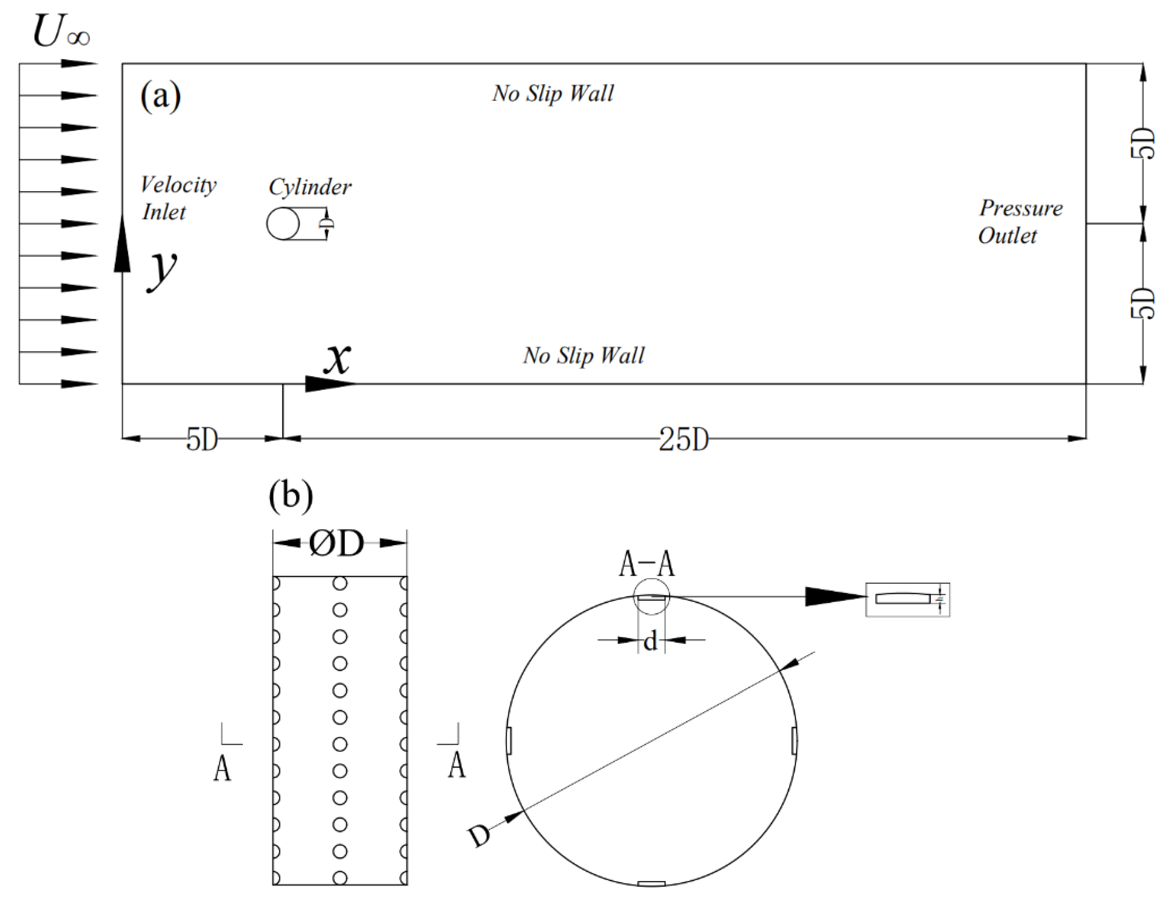
2.2. Computational Domains and Boundary Conditions

The numerical simulations carried out in this paper shared the same computational domain, as shown in Figure 1a. The domain size is determined based on the study by Sarker [17]. According to Sarker’s research, the distance from the flow field’s outlet to the cylinder’s center should be no less than 12D, which would ensure the disappearance of the cylinder’s influence on the fluid. To better observe the flow field’s backflow, the distance from the basin outlet to the center of the cylinder was set to 25D. The gap between the basin inlet and the cylinder’s center was 5D, and the distance between the cylinder’s center and the two sides of the wall was 5D. Finally, a rectangle computational domain of 30D (in the streamwise direction) × 10D (in the transverse direction) was adopted for 2D numerical simulations.

The boundary conditions of the computational domain are also known from Figure 1a. For all simulations, the flow field’s inlet and outlet are the velocity inlet boundary and the pressure outlet boundary, respectively. The front and back are no-slip walls, and the cylinder is a fixed wall boundary. The geometric model above uses the two-dimensional rectangular coordinate system for this computational domain. In this coordinate system, x and y denote the streamwise and transverse directions of the flow field. Figure 1b is a schematic diagram of the dimpled structure. D (D = 20 mm), h, and d are the cylinder’s diameter, dimple’s depth, and the dimple’s diameter (d = 2 mm, d/D = 0.1), respectively.

Table 1. Included cases of the numerical simulation.

Number of Columns	Re1 = 1 × 105	Re2 = 2 × 105
0 column	Case 1-1	Case 2-1
4 columns	Case 1-2	Case 2-2
8 columns	Case 1-3	Case 2-3
12 columns	Case 1-4	Case 2-4

provides the simulation cases and parameters covered. The number of dimple columns controlled the number of dimples. The dimples were evenly distributed on the surface of the cylinder in an equiangular manner. The distribution of dimples in four columns, for example, is given in Figure 1b. The relevant parameters of Re are obtained from the investigations [18,19,20,21]. The pile leg’s diameter was set as 0.5 m, and the environmental flow velocity of the pile leg was 0.2 m/s and 0.4 m/s. To sum up, the values of Reynolds number are Re₁ = 1 × 10⁵ and Re₂ = 2 × 10⁵, respectively. h is estimated by the formula of boundary layer thickness [22,23] (h = 0.035DRe − 1/7). To control the cylinder’s roughness, the value of k is equal to 0.1 mm. That is, k/D = 0.005 (k/D is the roughness coefficient, and k = h is the dimple’s depth).

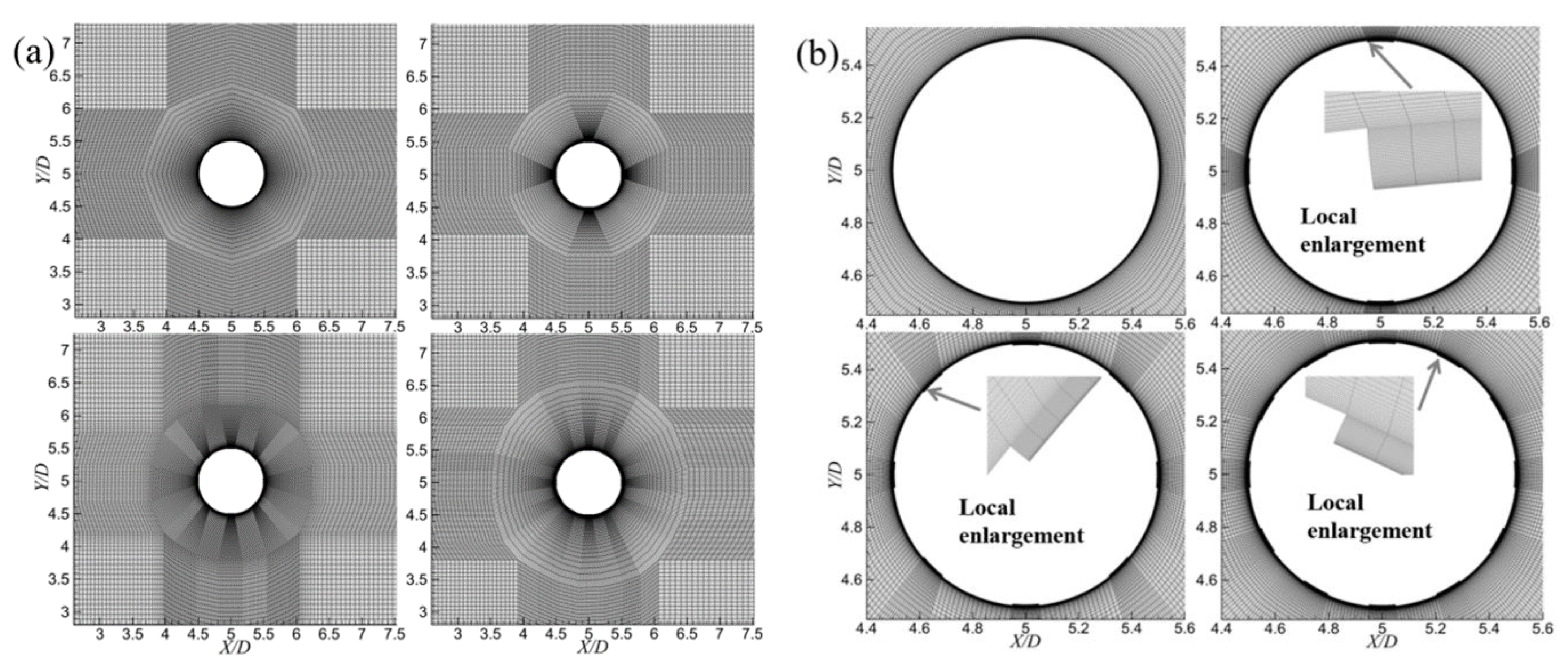
2.3. Computational Mesh

In the region near the cylindrical wall, the gradient of the average velocity is considerable. In a very short reasonable distance from the wall, the relatively large velocity value is suddenly reduced to the same velocity value as the wall. Due to such phenomena, the simulation of the flow around a cylinder needs treatment of the near-wall [22,24]. Since the Transition-SST turbulence model is adopted in this paper, it is usually required to meet y⁺ ≈ 1. The relation between y+ and the height of the first layer mesh can be expressed as [25]:

$$y^{+}=0.172\frac{\Delta y}{D}R{e}^{0.9}$$

(14)

Here, Δy is the height of the first layer mesh, and D is the cylinder’s diameter. Calculated by the formula, the height of the first layer mesh of the two models in this paper is 0.004 mm and 0.0021 mm. During the dividing of the grid, the height of the first layer mesh was set to 0.001 mm.

After finishing the above work, grid independence verification was undertaken. Four different meshes for the smooth cylinder and the dimple cylinder at Re = 1 × 10⁵ were checked. The number of cells was controlled by the grid expansion ratio and the number of nodes.

Table 2. Grid independence verification for the smooth cylinder at Re = 1 × 10⁵.

Mesh	Description		Number of Cells	Time-Averaged Drag Coefficient $\left(\overline{\mathit{C}\mathit{d}}\right)$	Root Mean Square of Lift Coefficient (Clrms)	Strouhal Number (St)
M1	The first layer height 0.00005D	Mesh expansion ratio of 1.3	72,936	1.4001	0.7492	0.2337
M2		Mesh expansion ratio of 1.2	89,476	1.3129	0.6391	0.2212
M3		Mesh expansion ratio of 1.1	107,116	1.2424	0.6217	0.2137
M4		Mesh expansion ratio of 1.05	125,856	1.2418	0.6214	0.2130

and

Table 3. Grid independence verification for the dimple cylinder at Re = 1 × 10⁵.

Mesh	Description		Number of Cells	Time-Averaged Drag Coefficient $\left(\overline{\mathit{C}\mathit{d}}\right)$	Root Mean Square of Lift Coefficient (Clrms)	Strouhal Number (St)
M1′	the first layer height 0.00005Ddensify 40 layers mesh for the location with dimples	Mesh expansion ratio of 1.3	96,988	1.3412	0.7115	0.2214
M2′		Mesh expansion ratio of 1.2	105,462	1.2584	0.7073	0.2206
M3′		Mesh expansion ratio of 1.1	110,302	1.0060	0.6131	0.2010
M4′		Mesh expansion ratio of 1.05	131,214	1.0052	0.6114	0.2005

summarize the verification results, providing the dependence of the $\overline{Cd}$ ($\overline{Cd}$ is the time-averaged drag coefficient. Cd = Fd/0.5ρU_∞²A, where Cd is the drag coefficient, Fd is the drag of the cylinder, ρ is the fluid density, U_∞ is the flow velocity, and A is the upwind area), and Cl_rms is the root mean square of lift coefficient. $C{l}_{rms}=\sqrt{\frac{{\displaystyle \sum _{m=1}^{N}C{l}_m^2}}{N}}=\sqrt{\frac{C{l}_1^2+C{l}_2^2+\cdots +C{l}_N^2}{N}}$), and the Strouhal number St (St = fD/U_∞, where f is the vortex shedding frequency, D is the cylinder diameter, U_∞ is the flow velocity) on the mesh size. The three values converged at M3 and M3′. It can be seen that the data differences between M3 and M4 or M3′ and M4′ are around 0.32%, indicating that a further increase of mesh resolution would have a negligible effect on the results of the numerical simulation [26]. In the end, the mesh size of M3 (for the smooth cylinder) and M3′ (for the dimple cylinder) was adopted in this simulation, the grid expansion ratio was kept below 1.1, and the time step size was controlled below 4 × 10⁻⁴ s. The results of the meshing are shown in Figure 2. For the smooth cylinder, this mainly controls the area with dense meshes, while for the cylinder with dimples, it is vital to separate the dimples separately for grid division.

2.4. Parameter Verification

The parameter verification was performed for the smooth cylinder at Re = 1 × 10⁵ to verify the accuracy of the turbulence model. The parameters include $\overline{Cd}$ and St, and the experimental data came from the research of Schewe [27] and Zdravkovich [28]. According to

Table 4. Comparison of related parameters.

Source of Literature	$\overline{\mathit{C}\mathit{d}}$	St	Note
Schewe	1.18	0.21	experiment
Zdravkovich	1.2	0.20	experiment
This paper	1.24	0.22	simulation

, the values of $\overline{Cd}$ and St in the numerical simulation are very close to the experimental values, indicating that the results of the turbulence model are highly reliable.

2.5. Numerical Simulation Parameters Setting

Based on the above work, the basic setup for fluid computing software can be selected as follows, as tabulated in

Table 5. The input parameters.

The Parameters	Choices	Notes
Solver	Pressure-Based, Transient
Model	Transition-SST
The fluid medium	Water-liquid (20°)	ρ = 998.2 kg/m3 μ = 0.001003 kg/(m·−s)
The boundary conditions	Velocity-Inlet & Pressure-Outlet
Pressure-Velocity Coupling Scheme	SIMPLEC
Spatial Discretization	Second Order Upwind

. In the table, it can be obtained that the solver is a pressure-based transient solver, the pressure-velocity coupling scheme is SIMPLEC, and the solution format is the second-order upwind format.

3. Numerical Simulation Results and Discussion

3.1. Drag Coefficient

The following formula can calculate the drag reduction rate:

$$\eta =\frac{{\overline{Cd}}_{smooth}-\overline{Cd}\mathrm{dimpled}}{{\overline{Cd}}_{smooth}}\times 100\%$$

(15)

Here, η is the drag reduction rate in the equation (“+” is for drag reduction, “−” is for drag increase). $\overline{Cd}$_smooth represents the time-averaged drag coefficient of the smooth cylinder, and $\overline{Cd}$_dimpled is the time-averaged drag coefficient of the circular cylinder with the dimpled surface.

Table 6. The drag reduction rates of included cases.

Serial Number	Remark	$\overline{\mathit{C}\mathit{d}}$	η
1	Case 1-1	1.242
2	Case 1-2	1.006	+19.00%
3	Case 1-3	1.088	+12.40%
4	Case 1-4	1.091	+12.16%
5	Case 2-1	0.898
6	Case 2-2	0.931	−3.67%
7	Case 2-3	1.060	−18.04%
8	Case 2-4	1.080	−20.27%

provides the drag reduction rates for all cases. For Re = 1 × 10⁵, compared to Case 1-1, it can be obtained that the $\overline{Cd}$ of Case 1-2, Case 1-3, and Case 1-4 is smaller, and the value of $\overline{Cd}$ increases in turn with the increase of the number of dimples. The maximum of η is +19.00% for Case 1-2, and the minimum of η is +12.16% for Case 1-4. However, at Re = 2 × 10⁵, $\overline{Cd}$ of Case 2-2, Case 2-3, and Case 2-4 is higher than that of Case 2-1. Similarly, $\overline{Cd}$ increases in turn with the increase in the number of dimples. The maximum of η reaches −20.27%.

The above results indicate that dimples can effectively reduce the cylinder drag within a certain Reynolds number. When the Reynolds number exceeds a certain critical value, dimples will bring about the opposite effect. Moreover, the number of dimples has a significant influence on the drag of the cylinder. A cylinder with more dimples adhering to its surface will create more considerable drag. In other words, the roughness of the cylinder surface will affect the drag of the cylinder.

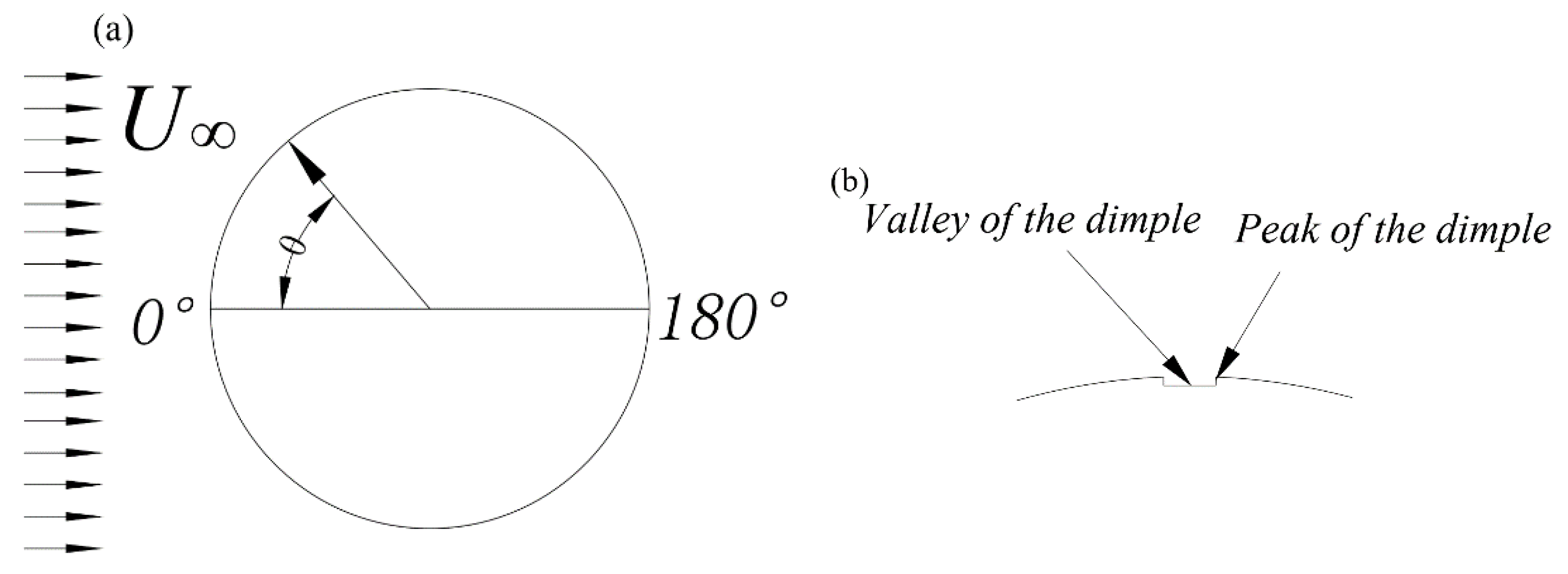
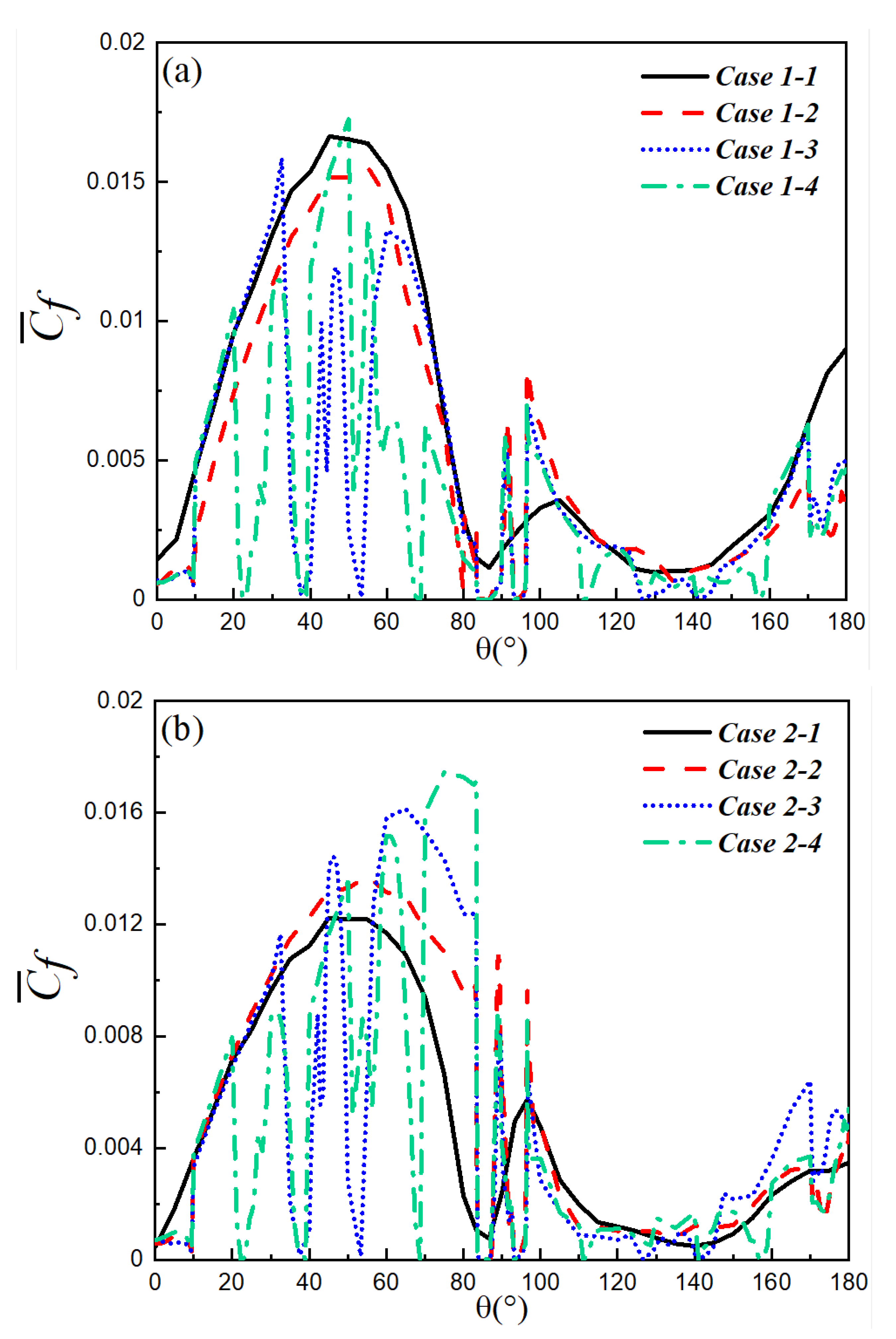
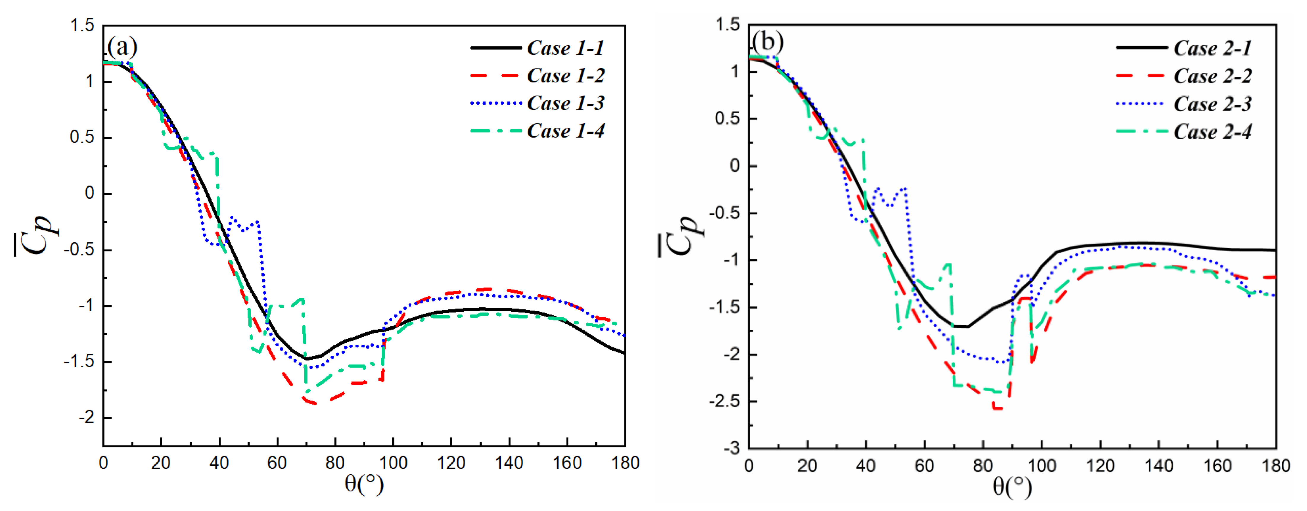
3.2. Pressure Coefficient and Skin Friction Coefficient

Previous studies [29] have shown that the smooth cylinder drag mainly comes from pressure drag (a component of the total drag), accounting for more than 98% of the full drag. However, for rough cylinders, the pressure drag and the skin friction drag are both critical [30], so the analysis of both is indispensable.

Figure 3a depicts a schematic sketch for monitoring the pressure coefficient and the skin friction coefficient. θ is the monitoring angle relative to the streamwise direction. The initial monitoring point is set at θ = 0°, and the angle ranges from 0° to 180° (along the streamwise path). Figure 3b shows the schematic sketch of a dimple. The dimpled interior can be regarded as the dimple valley, and the sharp edge can be viewed as the peak of the dimple [31].

Figure 4 and Figure 5 expose the time-averaged skin friction coefficient $\overline{Cf}$ (Cf = τ_ω/0.5ρU_∞², where τ_ω is the shear stress) and the time-averaged pressure coefficient $\overline{Cp}$ (Cp = (p_θ − p_∞)/0.5ρU_∞², where p_θ is the pressure at the rear stagnation points, and p_∞ is the reference pressure at the inlet). It is known that the skin friction drag is the integral of the shear stress on the cylinder surface, and the pressure along the cylinder surface can be integrated to obtain the pressure drag. Therefore, $\overline{Cf}$ and $\overline{Cp}$ can represent the skin friction drag and pressure drag on the cylinder surface.

At Re = 1 × 10⁵, as shown in Figure 4a, $\overline{Cf}$ first increases and then decreases with the increase of θ for Case 1-1 in the range of 0° < θ < 87° and reaches the maximum value at θ ≈ 50°. The curve of $\overline{Cf}$ for Case 1-1 is relatively smooth. However, for Case 1-2, Case 1-3, and Case 1-4, it is evident that the value of $\overline{Cf}$ will decrease sharply then increase suddenly at the dimple positions, and the minimum value is around 0. Other than that, at the same place on the cylinder surface, $\overline{Cf}$ of Case 1-2, Case 1-3, and Case 1-4 is greater than that of Case 1-1 (except for the location of 90° < θ < 120°). For this reason, the skin friction drag obtained by integrating on the circular cylinder with the dimpled surface is less than that of the smooth cylinder. When 90° < θ < 120°, there is a phenomenon of vortex reattachment, and the dimple will enhance this phenomenon, so $\overline{Cf}$ of the circular cylinder with the dimpled surface will be higher than that of the smooth cylinder.

For Re = 2 × 10⁵ (Figure 4b), $\overline{Cf}$ of Case 2-2, Case 2-3, and Case 2-4 is higher than that of Case 2-1 at the same location. The difference between Figure 4a,b indicates that the flow velocity also influences the drag of the circular cylinder with the same structure. Because of this phenomenon, the skin friction drag for the circular cylinder with the dimpled surface will be greater at Re = 2 × 10⁵. This difference is one of the essential reasons why the dimpled structure’s drag reduction results are different at the two Reynolds Numbers.

The curve characteristics of $\overline{Cp}$ are similar to that of $\overline{Cf}$ (Figure 5). For example, the curve of $\overline{Cp}$ for the smooth cylinder is relatively smooth. For the circular cylinder with the dimpled surface, $\overline{Cp}$ fluctuates wildly at the dimple positions. However, the pressure drag results for Re = 1 × 10⁵ and Re = 2 × 10⁵ are different. The pressure drag of the circular cylinders with the dimpled surface is lower than that of the smooth cylinder at Re = 1 × 10⁵ but higher than that of the smooth cylinder at Re = 2 × 10⁵.

From Figure 4 and Figure 5, it is concluded that both the number of dimples and the flow velocity have an effect on the total drag. In other words, at a certain Reynolds number interval, the proper roughness for the cylinder surface will reduce the cylinder drag.

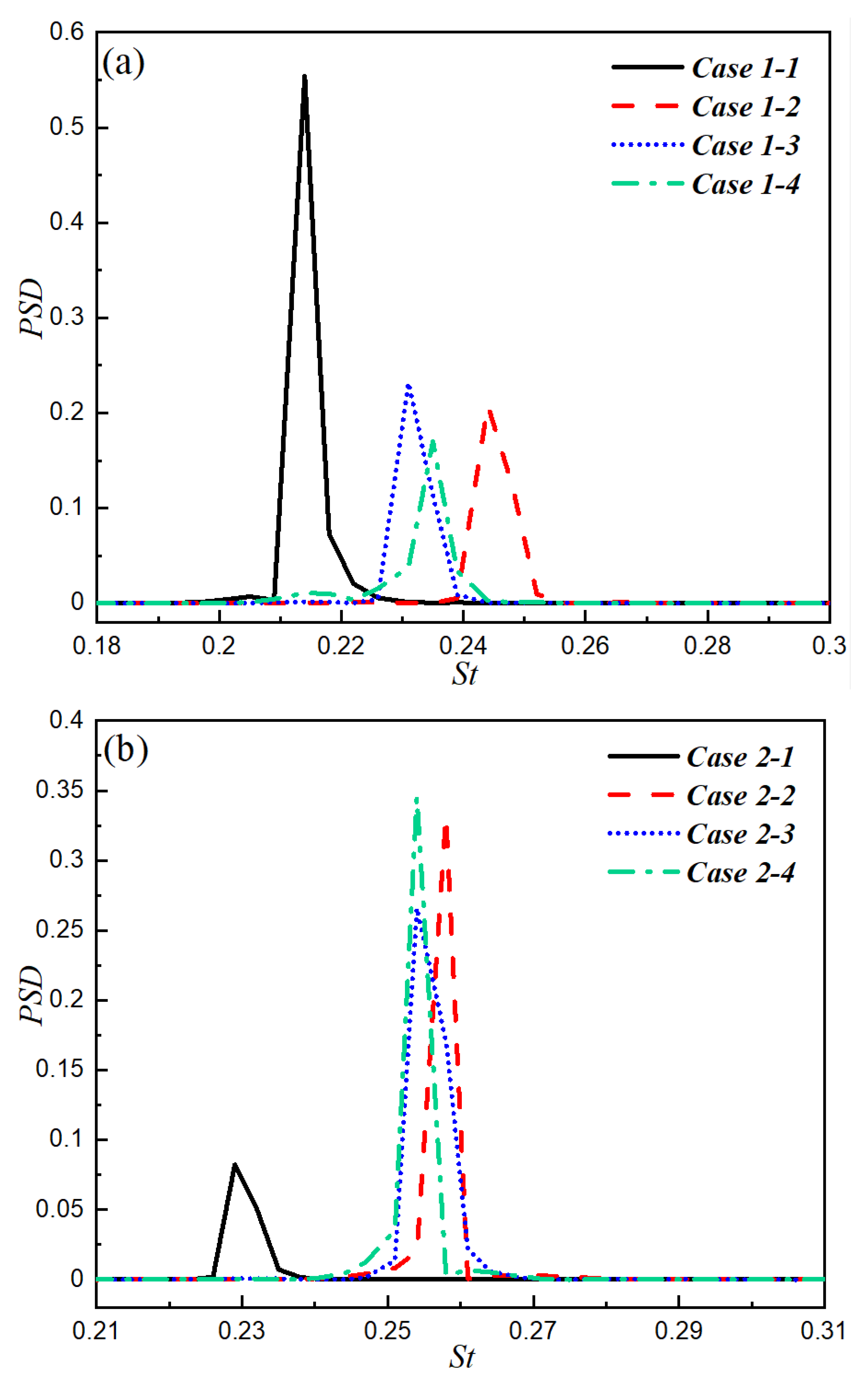
3.3. Vortex Shedding Strength

In this study, Fast Fourier Transforms (FFT) is used to analyze lift coefficient (Cl) and its calculation method can be described as follows.

For a periodic set of N sampled points, ${\varphi }_k$, the discrete Fourier transform [32] expresses the signal as a finite trigonometric series:

$${\varphi }_k={\displaystyle \sum _{n=0}^{N-1}{\widehat{\varphi }}_n}{e}^{2\pi ikn/N}\hspace{1em}k=0,1,2,\dots (N-1)$$

(16)

where the series coefficients ${\widehat{\varphi }}_n$ are computed as:

$${\widehat{\varphi }}_n=\frac{1}{N}{\displaystyle \sum _{k=0}^{N-1}{\varphi }_k}{e}^{-2\pi ikn/N}\hspace{1em}n=0,1,2,\dots (N-1)$$

(17)

In addition, Power Spectral Density (PSD) is the distribution of signal power in the frequency domain, and it is defined for the frequency f_n:

$$PSD\left(f_n\right)=E\left(f_n\right)/\Delta f\hspace{1em}n=1,2,\dots ,N/2$$

(18)

where Δf is the frequency step in the discrete spectrum, and the Fourier mode power E(f_n) is computed as:

$$E\left(f_n\right)=\{\begin{array}{cc}0.5{\left(2\left|{\widehat{\varphi }}_n\right|\right)}^2& n=1,2,\dots ,N/2-1\\ {\left|{\widehat{\varphi }}_n\right|}^2& n=N/2\end{array}$$

(19)

Figure 6 profiles the relationship between the PSD and the St (St = fD/U_∞, where f is the vortex shedding frequency, D is the cylinder diameter, and U_∞ is the flow velocity). As plotted in Figure 6a, at Re = 1 × 10⁵, it is evident that the peak values of PSD of Case 1-2, Case 1-3, and Case 1-4 are smaller than that of Case 1-1 [9,33], indicating that the dimpled structure can reduce the strength of vortex shedding. The distribution characteristics of the curve in Figure 6b are entirely different from those in Figure 6a, in that the peak values of PSD of Case 2-2, Case 2-3, and Case 2-4 are much higher than that of Case 2-1. It is conceivable that the dimpled structure will increase the strength of vortex shedding at Re = 2 × 10⁵. The advantage of vortex shedding will affect the structure of the flow field and the size of the vortex. Thus, it is a non-negligible factor influencing the drag of the cylinder.

4. Experimental Results and Discussion

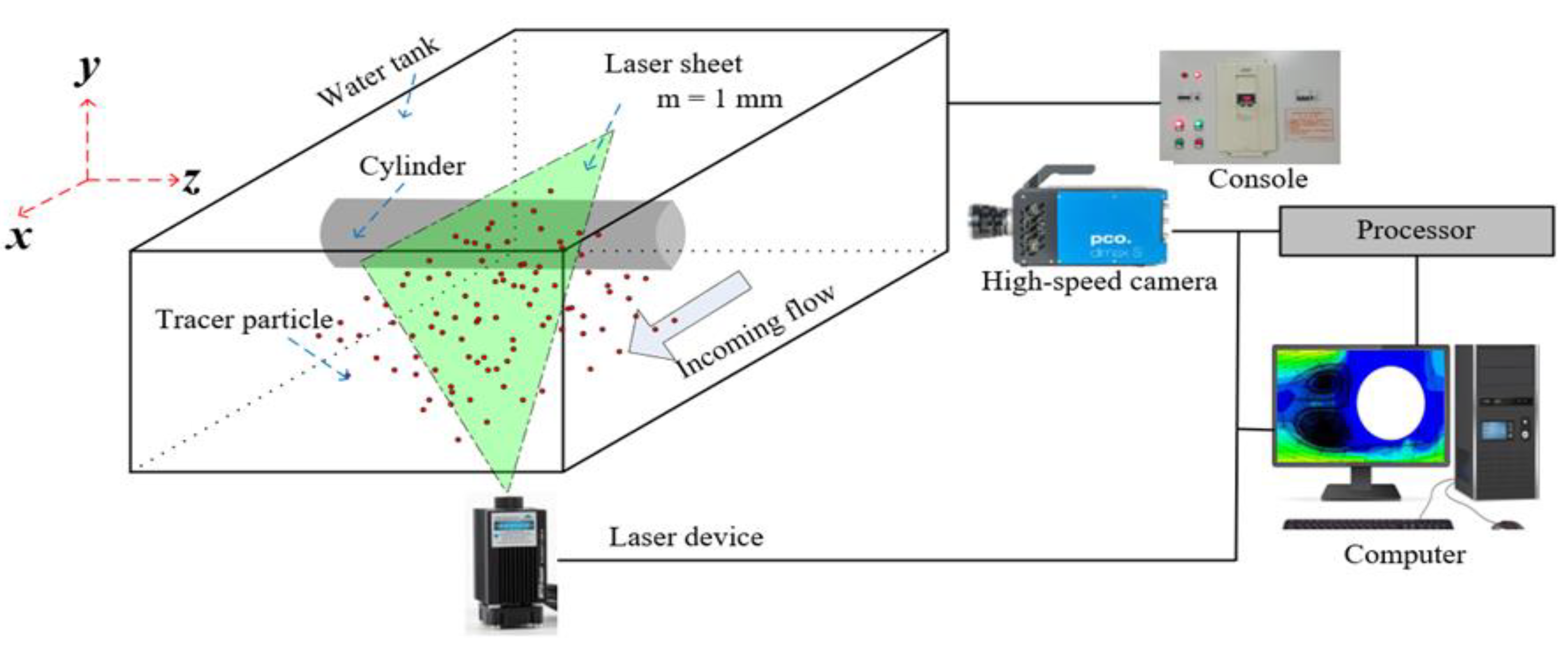
4.1. Experimental Equipment

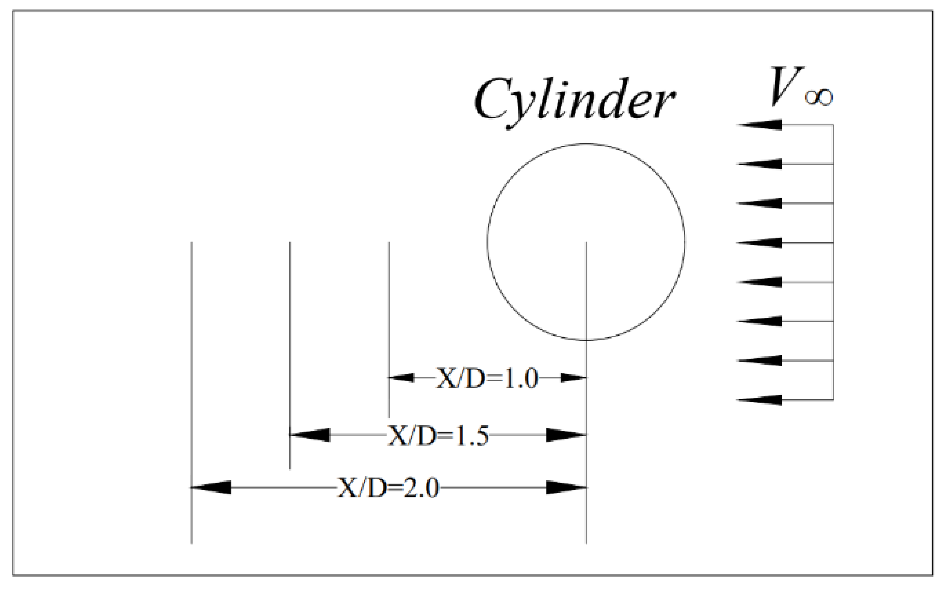
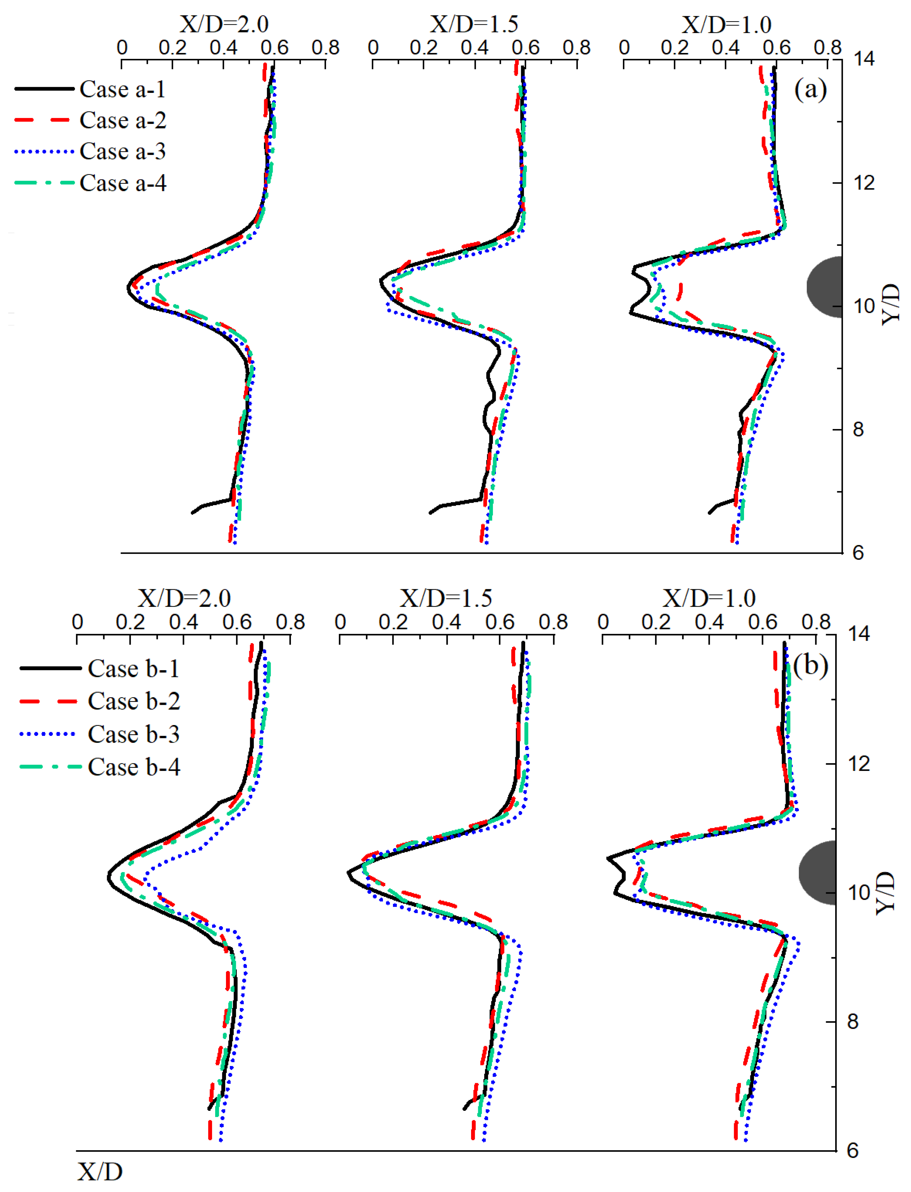
The PIV technique is used to display the flow around the cylinder with or without dimples to observe the field’s backflow. The circulating water tank is about 4 m long with a rectangular cross-section of 0.3 m × 0.25 m (width × height), so the cross-sectional area S of the tank in the experimental section is 0.075 m². An innovative bench was built based on the water tank and related experimental equipment, as presented in Figure 7. The console controls the quantity of flow, thus controlling the flow velocity. The schematic diagram also gives the flow direction. The two side walls and bottom surfaces of the tank are made of glass to facilitate the access of lasers generated by optical instruments.

The cylinders used in the experiment are made of aluminum, and the dimples are machined by the Computer Numerical Control (CNC) machining center. The length of the cylinders is 302 mm, and their diameter is 20 mm. The diameter (d) and depth (h) of the dimples are 2 mm (d/D = 0.1) and 0.1 mm (k = h = 0.1 mm, k/D = 5 × 10⁻³), respectively. The distance between two dimple centers is 4 mm, and the dimples are evenly distributed on the cylinder. Figure 8 provides the specific size data and finished product.

The length-to-diameter of the cylinders used in the experiment is 15.1, which is considered large enough to ensure a 2D flow of the cylinder’s near-wake [34]. The coordinates x, y, and z represent the streamwise, transverse, and spanwise directions, as shown in Figure 7. The flow velocity in the experiment is calculated according to the flow rate formula (Q = SV_∞, where Q is the quantity of flow, S is the cross-sectional area, and V_∞ is the flow velocity in the experiment). It is noteworthy that V_∞ is consistent with the environmental velocity of the pile leg. The two free-stream velocities in the experiment are 0.204 m/s and 0.407 m/s, corresponding to Re₁ = 4.08 × 10³ and Re₂ = 8.14 × 10³, respectively.

Table 7. Covered experimental conditions.

Q (m3/h)	S (m2)	V∞ (m/s)	Re
55	0.075	0.204	4.08 × 103
110		0.407	8.14 × 103

and

Table 8. Included test cases.

Number of Columns	Re1 = 4.08 × 103	Re2 = 8.14 × 103
0 column	Case a-1	Case b-1
4 columns	Case a-2	Case b-2
8 columns	Case a-3	Case b-3
12 columns	Case a-4	Case b-4

demonstrate the lists of test cases and experimental conditions.

Figure 7 also presents the experimental set-up of high-speed PIV. A high-speed camera (pco. dimax S1) with a resolution of 1008 × 1008 pixels was used to capture the 2000 successive digital particle images at a time interval of 1 ms (i.e., 1000 frame per second) between two consecutive images, and the shutter speed of each frame is set at 1.5 μs. A thin light-sheet of thickness m = 1 mm produced by a high-intensity continuous light source (Figure 7) was used to illuminate the tracer particles (the diameter of the tracer particle is 10 μm) around the cylinder. The distance from the camera’s focal plane mark to the light-sheet plane was fixed at about 0.5 m. The PIV view software based on the spatial cross-correlation method was applied to record the particle trajectories in the flow around a cylinder.

4.2. Velocity Field

As shown in Figure 9, to analyze the backflow velocity of cylinders in the experiment, the streamwise velocities of three locations close to the cylinder in the backflow region are extracted and compared. The measurements are performed at three different locations: X/D = 1.0 (location A), X/D = 1.5 (location B), and X/D = 2.0 (location C) from the center of the cylinder.

The averaged streamwise velocity ($\overline{U}$/V_∞) profiles in the near wake behind the cylinder are reported in Figure 10. According to Figure 10, it is apparent that the velocity curve shows a “U” shape near the cylinder, while the curve changes and presents a “V” shape away from the cylinder. These phenomena can also be found in the research of Aguedal et al. [35].

Under the premise that the streamwise velocity profile in the wake does not change significantly along the streamwise direction, these velocity profiles were used as stability analysis [36]. As shown in Figure 10a, it is interesting to note that Case a-2, Case a-3, and Case a-4 recover 22.34–36.58% of the incoming flow velocity at the location A (X/D = 1.0) while Case a-1 does not. The results indicate a lower dimpled structure velocity gradient and a lower shearing action than a smooth one [37]. However, this percentage is down to 24.15–8.45% at location C (X/D = 2.0). On the other hand, at Re = 8.14 × 10³ (Figure 10b), Case b-2, Case b-3, and Case b-4 show the higher momentum deficiency even at the location A (X/D = 1.0) and the velocity recovery is slower than is the case in Figure 10a. This phenomenon indicates that the increase of Reynolds number weakens the effect of dimples on velocity recovery.

4.3. Vortex Structure

Figure 11 depicts a schematic sketch of the recirculation zone. It concludes the features of the flow field and the parameters, describing the near-wake recirculation zone. The flow field’s primary function is the formation of a symmetrical recirculation zone in the cylindrical near wake (the length of the recirculation zone (L_R) is measured from the center of the cylinder along with the streamwise direction). The circumfluence zone consists of a pair of fixed vortices, which are generally equal in strength and opposite in the course of rotation. a is measured from the center of the cylinder to the center of the vortex, and b is the distance between the centers of the pair of vortices. After, the vortex will become asymmetrical and fall off the cylinder [38].

To analyze the differences of the above flow characteristics in the experimental cases, the streamlines and time-averaged velocity vector diagram are used to show these features intuitively and clearly, plotted in Figure 12. Moreover, the values of the three parameters (L_R, a, and b) are measured in detail, as shown in Figure 12.

Figure 12 visually shows the state of vortices, and the structure of vortices in all cases is consistent with the description in Figure 11. The distinctions between each case are mainly reflected in the values of L_R, a, and b. For example, at Re = 4.08 × 10³, it can be observed that the three parameter values of Case a-2, Case a-3, and Case a-4 are almost more significant than those of Case a-1. This phenomenon also occurs at Re = 8.14 × 10³. From the above discussions, it can be concluded that when the drag of the circular cylinder with the dimpled surface decreases at the same Reynolds number, the three parameters in the near-wake field (L_R, a, and b) will increase [39,40]. A reasonable conclusion can be made that the dimple structure delays the release of the vortex at a specific range of the Reynolds number. Therefore, the formation of the larger vortex leads to a decrease in the vortex shedding frequency, thus the drag is reduced.

Interestingly, Zhou et al. [10] found that L_R, a, and b of the non-smooth cylinders were smaller than that of a smooth cylinder in their study. This result is different from the experimental result of this study and the conclusion of Liu et al. [39]. The reason may be due to the different roughness, which changes the influence of the boundary layer on the flow field.

The variation of the three parameters is provided in Figure 13 to compare the flow field in the numerical simulation and the experiment. It can be found that three parameter values in the numerical simulation always fluctuate above and below the experimental values, and the average error is about 2.7%. This result further demonstrates that the numerical simulation is credible.

5. Conclusions

In this paper, dimples with roughness coefficient k/D = 0.005 are arranged on the cylinder. The force coefficient, vortex shedding strength, velocity field, and vortex structure of different cylinders are analyzed. The following conclusions can be drawn from the above discussions:

(1)

The dimple structure can effectively reduce the drag of the cylinder within a specific range of Reynolds numbers. The maximum drag reduction rate reaches 19%. However, the drag reduction rate is reduced to a minimum of 12.16% with the increase in the number of dimples.

(2)

In terms of the composition of drag, it is also worth noting that both the pressure drag and the skin friction drag have an essential influence on the total drag of the circular cylinder with the dimpled surface.

(3)

When the drag is reduced, the cylinder’s vortex shedding strength is less than that of a smooth cylinder at the same Reynolds number. On the other hand, the drag of the circular cylinder with the dimpled surface will be increased when the flow velocity exceeds a certain critical value and the vortex shedding strength of the cylinders will be more muscular than that of the smooth cylinder.

(4)

The velocity recovery of the circular cylinder with the dimpled surface is faster than that of the smooth cylinder, indicating a lower velocity gradient and a lower shearing action in the dimpled structure. At the same time, the increase of Re will weaken the effect of dimples on velocity recovery.

(5)

Through discussions of the vortex scale, it is found that when the drag of the cylinder decreases, the values of L_R, a, and b will increase. This phenomenon indicates that the release of the vortex is delayed, and the drag of the cylinder is therefore reduced.

References

1. Muddada, S.; Patnaik, B.S.V. Active flow control of vortex induced vibrations of a circular cylinder subjected to non-harmonic forcing. Ocean Eng. 2017, 142, 62–77. [Google Scholar] [CrossRef]
2. Owen, J.C.; Bearman, P.W. Passive control of VIV with drag reduction. J. Fluid Struct. 2001, 15, 597–605. [Google Scholar] [CrossRef]
3. Ivo Amilcar, V.C.M.T. Experimental Investigation on Vortex Induced Vibrations of Bio-Cylinders Based on a Harbor Seal Vibrissa. Master’s Thesis, Harbin Institute of Technology, Harbin, China, June 2018. [Google Scholar]
4. Wang, F.H.; Jiang, G.D.; Luo, X.L. Experimental investigation on drag reduction of wavy cylinder in cross flow. J. Xi’an Jiaotong Univ. 2006, 40, 93–96. [Google Scholar]
5. Mohammadi, A.; Floryan, J.M. Groove optimization for drag reduction. Phys. Fluids 2013, 25, 113601. [Google Scholar] [CrossRef]
6. Ge, M.W.; Fang, L.; Liu, Y.Q. Drag reduction of wall bounded incompressible turbulent flow based on active dimples/pimples. J. Hydrodyn. 2017, 29, 261–271. [Google Scholar] [CrossRef]
7. Oki, M.; Suehiro, M.; Okanaga, H. Flow around a circular cylinder with and without grooves. Flow Vis. 1992, 327–332. [Google Scholar] [CrossRef]
8. Takayama, S.; Aoki, K. Flow characteristics around a rotating grooved circular cylinder with grooved of different depths. J. Vis. 2005, 8, 295–303. [Google Scholar] [CrossRef]
9. Zhou, B.; Wang, X.K.; Guo, W. Control of flow past a dimpled circular cylinder. Exp. Therm. Fluid Sci. 2015, 69, 19–26. [Google Scholar] [CrossRef]
10. Zhou, B.; Wang, X.K.; Guo, W. Experimental study on flow past a circular cylinder with rough surface. Ocean Eng. 2015, 109, 7–13. [Google Scholar] [CrossRef]
11. Wang, G.R.; Liao, C.J.; Hu, G. Numerical simulation analysis and the drag reduction performance investigation on circular cylinder with dimples at subcritical Reynolds number. J. Mech. Strength 2017, 39, 1119–1125. [Google Scholar]
12. Lei, J.M.; Tan, Z.M. Numerical simulation for flow around circular cylinder at high Reynolds number based on Transition SST. J. Beijing Univ. Aeronaut. Astronaut. 2017, 43, 207–217. [Google Scholar]
13. Shi, S.J.; Huo, J.B.; Zhan, J.Z. Study on airfoil surface flow based on transition model of γ-Reθt. J. Guilin Univ. Aerosp. Technol. 2018, 23, 334–338. [Google Scholar]
14. Langtry, R.B.; Menter, F.R. Correlation-based transition modeling for unstructured parallelized computational fluid dynamics codes. AIAA J. 2009, 47, 2894–2906. [Google Scholar] [CrossRef]
15. Langtry, R.B.; Menter, F.R.; Likk, S.R. A correlation-based transition model using local variables-part II: Test cases and industrial applications. J. Turbomach. 2006, 128, 423–443. [Google Scholar] [CrossRef]
16. Menter, F.R.; Langtry, R.B.; Likk, S.R. A correlation-based transition model using local variables-part I: Model formulation. J. Turbomach. 2006, 128, 413–422. [Google Scholar] [CrossRef]
17. Sarker, M.A. Flow measurement around scoured bridge piers using Acoustic-Doppler Velocimeter (ADV). Flow Meas. Instrum. 1998, 9, 217–227. [Google Scholar] [CrossRef]
18. Bai, A.P.; Mai, Y.F. Study on dynamic response of self-sustaining conditions of jack-up offshore platform pile leg storm based on ANSYS. China Water Transp. 2017, 7, 162–164. [Google Scholar]
19. Wang, Q. Strength and Fatigue Analysis of Jack-Up Platform Leg. Master’s Thesis, Harbin Engineering University, Harbin, China, May 2013. [Google Scholar]
20. Xu, J.H. The Research of Jack-Up Platforms in the Dynamic Response and Fatigue Analysis. Master’s Thesis, South China University of Technology, Guangzhou, China, June 2014. [Google Scholar]
21. Guo, X.Y. Research on the Adaptability of Working Water Depth of Jack-Up Platform Leg Structure Type. Master’s Thesis, Dalian University of Technology, Dalian, China, May 2017. [Google Scholar]
22. Fang, Y. Study on Drag Reduction of Revolution Body with Dimple and Convex Tubercle. Master’s Thesis, Beijing Jiaotong University, Beijing, China, July 2012. [Google Scholar]
23. Gu, Y.Q.; Zhao, G.; Zheng, J.X.; Li, Z.; Liu, W.; Muhammad, F. Experimental and numerical investigation on drag reduction of non-smooth bionic jet surface. Ocean Eng. 2014, 81, 50–57. [Google Scholar] [CrossRef]
24. Zhao, J. Study of Drag Reduction Capability of the Dimple Bionic Non-Smooth Surface. Master’s Thesis, Dalian University of Technology, Dalian, China, December 2008. [Google Scholar]
25. Chen, J.T. 2D numerical simulation and wake analysis on flow around circular cylinder. Comput. Aided Eng. 2013, 22, 1–6. [Google Scholar]
26. Zhu, H.J.; Zhou, T.M. Flow around a circular cylinder attached with a pair of fin-shaped strips. Ocean Eng. 2019, 190, 106–484. [Google Scholar] [CrossRef]
27. Schewe, G. On the force fluctuations acting on a circular cylinder in crossflow from subcritical up to transcritical Reynolds numbers. J. Fluid Mech 1983, 133, 265–285. [Google Scholar] [CrossRef]
28. Zdravkovich, M.M. Review and classification of various aerodynamic and hydrodynamic means for suppressing vortex shedding. J. Wind Eng. Ind. Aerodyn. 1981, 7, 145–189. [Google Scholar] [CrossRef]
29. Achenbach, E. Distribution of local pressure and skin friction around a circular cylinder in cross-flow up to Re = 5 × 10⁶. J. Fluid Mech. 1968, 34, 625–639. [Google Scholar] [CrossRef]
30. Sumer, B.M.; FredsØe, J. Hydrodynamics around Cylindrical Structures; World Scientific: Singapore, 1997. [Google Scholar]
31. Alonzo-GarcÍa, A. RANS simulations of the U and V grooves effect in the subcritical flow over four rotated circular cylinders. J. Hydrodyn. Ser. B 2015, 27, 569–578. [Google Scholar] [CrossRef]
32. Bracewell, R.N. The Fourier Transform and Its Applications; McGraw-Hill: New York, NY, USA, 1986. [Google Scholar]
33. Yokoi, Y.; Igarashi, T.; Hirao, K. The study about drag reduction of a circular cylinder with grooves. J. Fluid Sci. Technol. 2011, 6, 637–650. [Google Scholar] [CrossRef]
34. Szepessy, S.; Bearman, P.W. Aspect ratio and end plate effects on vortex shedding from a circular cylinder. J. Fluid Mech. 1992, 234, 191–217. [Google Scholar] [CrossRef]
35. Aguedal, L.; Semmar, D.; Berrouk, A.S.; Azzi, A.; Oualli, H. 3D vortex structure investigation using large eddy simulation of flow around a rotary oscillating circular cylinder. Eur. J. Mech.-B/Fluids 2018, 71, 113–125. [Google Scholar] [CrossRef]
36. Baek, H.; Karniadakis, G.E. Suppressing vortex-induced vibrations via passive means. J. Fluids Struct. 2009, 25, 848–866. [Google Scholar] [CrossRef]
37. El-Makdah, A.M.; Oweis, G.F. The flow past a cactus-inspired grooved cylinder. Exp. Fluids 2013, 54, 1464. [Google Scholar] [CrossRef]
38. Tonui, N.; Sumner, D. Temporal development of the wake of a non-impulsively started circular cylinder. In Proceedings of the ASME Fluids Engineering Division Summer Meeting, Vail, CO, USA, 2–6 August 2009. [Google Scholar]
39. Liu, Y.Z.; Shi, L.L.; Yu, J. TR-PIV measurement of the wake behind a grooved cylinder at low Reynolds number. J. Fluids Struct. 2011, 27, 394–407. [Google Scholar] [CrossRef]
40. Babu, P.; Mahesh, K. Aerodynamic loads on cactus-shaped cylinders at low Reynolds numbers. Phys. Fluids 2008, 20, 035112. [Google Scholar] [CrossRef] [Green Version]
Figure 1. The schematic diagrams of the computational domain and the cylinder: (a) Computational domain; (b) The distribution of four columns of dimples on the surface of the cylinder.
Water 13 00197 g001
Figure 2. Schematic diagrams of the mesh: (a) Computational grid; (b) Close-up of the grid around the cylinder.
Water 13 00197 g002
Figure 3. The schematic sketches: (a) Force coefficient monitoring angle; (b) Close-up of the dimple.
Water 13 00197 g003
Figure 4. Distribution of time-averaged skin friction coefficient over the cylinder surface with different dimpled numbers: (a) Re = 1 × 10⁵; (b) Re = 2 × 10⁵.
Water 13 00197 g004
Figure 5. Distribution of time-averaged pressure coefficient over the cylinder surface with different dimpled numbers: (a) Re = 1 × 10⁵; (b) Re = 2 × 10⁵.
Water 13 00197 g005
Figure 6. Power Spectral Density of lift coefficient of the cylinders with different dimple numbers: (a) Re = 1 × 10⁵; (b) Re = 2 × 10⁵.
Water 13 00197 g006
Figure 7. Experimental setup in the water tank.
Water 13 00197 g007
Figure 8. Experimental cylinder: (a) cylinder size; (b) finished product.
Water 13 00197 g008
Figure 9. Position diagram for velocity distribution.
Water 13 00197 g009
Figure 10. Time-averaged streamwise velocity distribution of the experiment at different positions with different dimpled numbers: (a) Re = 4.08 × 10³; (b) Re = 8.14 × 10³.
Water 13 00197 g010
Figure 11. A schematic sketch of the recirculation zone.
Water 13 00197 g011
Figure 12. Time-averaged streamlines and mean streamwise velocity contours of the experiment.
Water 13 00197 g012
Figure 13. Variation of the normalized length scales of the cylinders with respect to Re: (a) the smooth cylinder; (b) the cylinder with 4 columns of dimples; (c) the cylinder with 8 columns of dimples; (d) the cylinder with 12 columns of dimples.
Water 13 00197 g013