Article

Modeling of Cavitation Bubble Cloud with Discrete Lagrangian Tracking

1
Department of Mechanical Engineering, Technical University of Munich, 85748 Garching, Germany
2
Siemens Limited China, Beijing 100102, China
*
Author to whom correspondence should be addressed.
These authors contributed equally to this work.
Water 2021, 13(19), 2684; https://doi.org/10.3390/w13192684
Submission received: 25 August 2021 / Revised: 20 September 2021 / Accepted: 24 September 2021 / Published: 28 September 2021
(This article belongs to the Special Issue Numerical Modeling and Simulation of Multi-Phase Flows)

Abstract

:
In this paper, a Lagrangian-Eulerian (LE) two-way coupling model is developed to numerically study the cavitation bubble cloud. In this model, the gas-liquid mixture is treated directly as a continuous and compressible fluid and the governing equations are solved by methods in Eulerian descriptions. An isobaric closure exhibiting better consistency properties is applied to evaluate the pressure of gas-liquid mixture. The dispersed gas/vapor bubbles are tracked in a Lagrangian fashion, and their compression and expansion are described by a modified Rayleigh-Plesset equation, which considers the close-by flow properties other than these of the infinity for each bubble. The performance of the present method is validated by a number of benchmark tests. Then, this model is applied to study how the bubble cloud affects the shape and propagation of a pressure wave when the pressure pulse travels through. In the end, a three-dimensional simulation of a vapor cloud’s Rayleigh collapse is carried out, and the induced extreme pressure is discussed in detail. The total bubble number’s influence on the extreme collapse pressure and the size distribution of bubbles during the collapse are also analyzed.

1. Introduction

Dispersed flows are characterized by one dispersed phase distributing within another continuous carrier phase in the form of solid particles, fluid droplets, or gas bubbles. Typical examples include solid particles suspending in gas or liquid, atomized drops in gas, and bubbly flow with dispersed gas/vapor bubbles. Dispersed flows are common and of great importance in various industrial and medical processes, e.g., fluid mixing and cleaning, sonochemical applications, and drug- and gene-delivery strategies [1,2,3,4,5,6]. In this paper, the flow cavitation, which has been investigated in diagnostic ultrasound treatment and chemistry processes [3,4,7], is studied, with a focus on the flows with cavitation bubble clouds.
Cavitation occurs when the static pressure of a liquid is decreased under the vapor pressure, which leads to the formation of vapor-filled cavities in the liquid. Violent collapse of these cavitation bubbles can induce damages to devices in engineering applications, such propellers, liquid fuel injectors, and turbines, which is considered as the main event contributing to the destructive influence of cavitation [8,9,10]. When a bubble collapses violently, the resulting shock wave can induce noise and destroy the surfaces of nearby equipment. Thus, cavitation is usually undesirable and should be avoided in engineering design processes. However, cavitation also plays a positive role in many medical applications [4,11]; for example, the treatment efficiency in high-intensity focused ultrasound (HIFU) surgery can be improved by using cavitation bubble clouds.
Over the past few decades, computational fluid dynamics (CFD) has become an indispensable tool in engineering and science to investigate complex practical problems. Although experiments may provide critical insights into the phenomena of bubble cloud cavitation [12,13,14], CFD can give precise measurement for individual bubbles, which is a challenging task by experiment due to the fast dynamic of bubble oscillations under small spatial scale. In recent years, many problems regarding cavitation have been studied numerically, e.g., shock wave propagation in bubbly flow [15,16], bubbly flow turbulence [17,18], and bubble cloud in an acoustic field [19,20].
Nevertheless, numerical modeling of cavitation flow is challenging due to the polydispersity of cavitation bubbles which ranges from dilute to dense. In general, gas-liquid interfaces can be classified into fully solved (resolved), under-resolved, and sub-grid interfaces with respect to grid size. A schematic of three different interface types is given in Figure 1. Various of numerical methods, such as those in References [9,21], have been developed to model the resolved and under-resolved interfaces. In this work, the sub-grid bubble-fluid interface is mainly considered, and the Lagrangian-Eulerian (LE) coupling model is adopted.
The LE coupling model includes the Lagrangian tracking of dispersed bubbles, the Eulerian description of carrier fluids, and an LE coupling scheme [20,22,23]. By this model, the dynamics of each bubble and that of the bubble-scattered pressure wave can be accurately captured with an acceptable computational cost [24]. Besides, this model is capable of taking into account the effect of non-uniform spatial distribution of bubbles on shock propagation and mimicking the experimental conditions, which is essential for both numerical and theoretical analysis [14]. Generally, LE coupling scheme can be classified into two groups according to the coupling approach, i.e., one-way and two-way couplings. In one-way coupling, the influence of the carrier phase on the dynamics of the dispersed phase is assumed to be the dominant effect [25]. When the mass of the dispersed phase is comparable with that of the carrier phase, the backward influence, that of the dispersed phase on the carrier phase, cannot be ignored anymore, and a two-way coupling is needed. In addition, the advection of the gas volume fraction and the pressure closure of the gas-liquid mixture are still challenging and remain open questions [20,23,26].
In this paper, we propose an LE two-way coupling model to study the cavitation bubble cloud. The isobaric closure, which has better mathematical properties regarding consistency and hyperbolicity than the isothermal closure [21], is applied. The gas-liquid mixture is treated as a compressible fluid with pressure equilibrium and solved in Eulerian frame. The dispersed bubbles move passively with the bulk fluid, and their dynamics are described by a modified Rayleigh-Plesset (RP) equation. The equilibrium pressure will be consequently applied to formulate the nearby flow properties in the modified RP equation, which allows the fluid surrounding each bubble be physically modeled. After validating this model by several benchmark cases, we apply it to study two practical problems, i.e., pressure wave interacting with a cavitation bubble cloud and Rayleigh collapse of a bubble cloud. The remainder of this paper is organized as follows. Section 2 describes the details of the proposed model. The corresponding numerical methodologies for the model and related equations are introduced in Section 3. Section 4 presents three benchmark test cases for validation. Two applications are then given in Section 5 and Section 6, respectively, and concluding remarks are drawn in Section 7.

2. LE Two-Way Coupling Model

In the present LE two-way coupling model, the cavitation fluid mixture is assumed to be a homogeneous compressible fluid solved in Eulerian framework, while each individual bubble in the cavitation bubble cloud is modeled using Lagrangian discrete tracking. In addition, we assume that bubbles do not significantly influence the momentum or the velocity of the mixture; thus, the bubble, carrier liquid and mixture are set to share the same local velocity. The effect of bubbles on the flow is considered by varying the mixture density and the pressure field due to their convection and mixing with the carried liquid. In this section, the coupling model-related equations, including the governing equations, the gas volume fraction, and fluid mixture models, are presented.

2.1. Governing Equations

In Eulerian description, the governing equation for inviscid and compressible gas-liquid mixture yields
U t + · F U = 0 ,
where U = [ ρ , ρ u , E ] T is the vector of conservative variables, and F = [ ρ u , ρ u u + p δ , u ( E + p ) ] T represents the flux vector. Here, ρ denotes the density, u the velocity, p the equilibrium pressure of the mixture, δ the unit matrix, and E = ρ e + ρ u · u 2 is the total energy. By introducing the liquid and gas volume fractions α l and α g , the mixture density and internal energy during gas-liquid mixing have the following expressions:
ρ = α l ρ l + α g ρ g ρ e = α l ( ρ e ) l + α g ( ρ e ) g 1 = α l + α g ,
where the subscripts l and g denote the carrier liquid and the gas bubbles, respectively.
Without taking account the bubble fission and coalescence, the motion of each dispersed bubble is tracked by
d x b d t = u ( x b ) ,
where b is the bubble index, and u ( x b ) is the local velocity of the fluid mixture. Following the classical RP equation [27,28], dynamics of a spherical bubble surrounded by a weakly compressible liquid at infinite can be expressed as
ρ R d 2 R d t 2 + 3 2 d R d t 2 = p B p 2 S R 4 μ R d R d t ,
where R is bubble radius, S surface tension, μ viscosity, and p denotes the far-field pressure of the surrounding fluid. Note that only the influence from surrounding fluid is involved in the dynamics, and the bubble-bubble interaction is not considered. As a cavitation bubble always contains vapor and some quantity of contaminant gas, we denote p v as the vapor pressure, and p g 0 as the pressure of contaminant gas at a reference bubble size R 0 . When the bulk fluid’s temperature at infinity T stays constant, p v is considered constant, too. p B is the pressure inside the bubble and has the following expression:
p B = p v + p g 0 R 0 R 3 γ g .
To close the system of governing equations in Equation (1), the gas volume fraction and the fluid-mixture pressure are needed.

2.2. Gas Volume Fraction

One key function of the LE coupling scheme is the formulation of the gas/vapor volume fraction α g distribution derived from the size and location of the instantaneous bubbles. Following References [20,26,29], we adopt a truncated Gaussian kernel function
ζ σ x x b = 1 σ 2 π d exp x x b 2 2 σ 2 | x x b | 3 σ 0 | x x b | > 3 σ ,
where d is the space dimension, and σ is the kernel width. Here, 3 σ is set as the cut-off radius according to numerical experiments for the purpose of saving computational effort and ensuring sufficient accuracy. To enforce mass conservation, the kernel function is normalized over the entire domain by
Ω ζ σ x x b d V = 1 ,
where Ω is the entire domain. With the kernel function, the explicit expression of gas volume fraction gives
α g x = i = 1 N b R b i ζ σ x , x b if n = 1 α g x = i = 1 N b π R b i 2 ζ σ x , x b if n = 2 α g x = i = 1 N b 4 3 π R b i 3 ζ σ x , x b if n = 3 ,
where N b is the total number of the dispersed bubbles within the cut-off radius, and R b i is the radius of bubble i.

2.3. Fluid-Mixture Pressure

An isobaric closure is applied to obtain the fluid-mixture pressure p. To avoid numerical oscillation near the interfaces [21], such closure must have the consistency properties: (a) the mixing of two fluids with the same pressure should maintain a mechanical equilibrium, and (b) the mixture pressure should degenerate correctly when one phase is vanishing. Here, we apply the stiffened-gas EOS to model p l and p g , which gives
p i = γ i 1 ρ i e i γ i B i ,
involving adiabatic exponent γ and reference pressure B for each fluid i. For gas bubbles, we take γ g = 1.4 and B g = 1 atm; for carrier water, γ l = 5.5 and B l = 492 atm. By introducing ξ g = 1 γ g 1 , ξ l = 1 γ l 1 , and ξ = α l ξ l + α g ξ g , an implicit expression for p is given as [30,31]
ρ e = p ξ + α l γ l B l ξ l + α g γ g B g ξ g ,
which yields the equilibrium pressure
p = ρ e ξ 1 ξ α l γ l B l ξ l + α g γ g B g ξ g .
It can be observed that Equation (11) satisfies the consistency properties. In addition, note that such pressure closure has been used for the numerical modeling of multi-component flows with immiscible interface to obtain the fluid pressure in the near-interface region [30,32].

3. Numerical Methods

In this section, numerical formulations for discretizing the LE two-way coupling model, including spatial discretization and time integration, are presented.

3.1. Bubble Dynamics

To avoid numerical oscillations, the truncated Gaussian distribution function as in Equation (8) is implemented for the gas volume fraction calculation in the mapping from Lagrangian frame to Eulerian frame. Note that bubbles may be several times larger than their initial sizes during the simulation; therefore, a constant kernel width σ cannot satisfy the needs that the volume fraction should be sufficiently smooth at each time step. To ensure that the interfaces are fully diffused in neighbor cells and avoid a negative volume fraction, the kernel width σ should be larger than the grid size and the maximum bubble radius, i.e.,
σ > max max R b i , d x ,
where dx is the grid size at the finest level of the multi-resolution mesh [33]. In addition, note that the restrictions of distance between bubbles, which should be larger than a characteristic distance, is not imposed in this model, allowing the overlap of the kernel widths of different bubbles. Thus, a pressure wave can only be resolved if its length is greater than σ . Otherwise, the pressure wave will be merged.
In classic RP equation as Equation (4), the radius R of a spherical bubble is defined by the pressure inside bubble p B and the infinity flow properties, i.e., p and ρ . However, defining the reference p and ρ of the surrounding liquid at infinity as p and ρ to model bubble cloud dynamics other than a single bubble is not suitable. To obtain p and ρ in Equation (4) for a bubble cloud, we define the fluid surrounding each bubble inside a limited volume V s as fluid mixture. The volume V s should enclose the bubble and be larger than the kernel support area [20]. According to numerical tests, we suggest 6 σ as the radius and the volume is marked by | x k x b | 6 σ . For bubble i, p and ρ have the following explicit expressions:
p = 1 V s V s p d V ρ = 1 V s V s ρ d V .

3.2. Spatial Discretization

We briefly describe here the spatial discretization of governing equations Equation (1). For simplicity, we consider the following one-dimensional hyperbolic conservation law
q t + f ( q ) x = 0 ,
where q ( x , t ) = ( ρ , ρ u , E ) T , and f ( q ) = ( ρ u , ρ u 2 + p , u ( E + p ) ) T . On a uniform grid, we denote x i = i Δ x , where Δ x is the grid spacing, and [ x i 1 / 2 , x i + 1 / 2 ] a computational cell i. Thus, Equation (14) on grids yields a system of ordinary differential equations (ODEs), which gives
d q i d t = f ( q ) x | x = x i , i = 0 , 1 , , n .
Here, the collocated finite volume (FV) scheme is applied, and the cell average value q ˜ i of a variable q is defined as
q ˜ i = 1 Δ x x i 1 / 2 x i + 1 / 2 q d x .
Equation (15) in cell i can be reformulated as
d q ˜ i d t = 1 Δ x f i + 1 / 2 f i 1 / 2 ,
where f i ± 1 / 2 is the approximated flux at the cell edge i ± 1 / 2 . The cell average value q ˜ i is applied to further do the reconstruction on each cell edge q i + 1 / 2 . A stencil involving several neighboring cells q ˜ i k , , q ˜ i + l is used for the reconstruction. Note that the reconstruction is required to be high-order accurate in smooth region and be essentially non-oscillatory (ENO) near discontinuities. In this work, the 5th-order weighted essentially non-oscillatory (WENO) scheme [34] is adopted, and the reconstruction is performed in characteristic space. Specifically, the variables are first locally decomposed onto the characteristic field and then reconstructed; afterwards, they are projected back into the physical field [35].
Normally, in FV reconstruction, the conservative variables q ˜ i are reconstructed to derive the left and right states of the conservative values q i + 1 / 2 L and q i + 1 / 2 R . However, numerical oscillations may present if the pressure p i + 1 / 2 is evaluated by the total energy E i + 1 / 2 and ξ i + 1 / 2 at cell edges in Equation (11) where isolated subgrid interfaces exit. After reconstructing the total energy E i + 1 / 2 and ξ i + 1 / 2 within the stencil, the pressure equilibrium will not be maintained. To address this problem, the primitive variables, instead of the conservative ones q ˜ i , are reconstructed for maintaining the pressure equilibrium [36]. Thus, at each time step in our methodology, we first build the cell-average primitive variables o ˜ i = ( ρ ˜ i , u ˜ i , p ˜ i , ξ i ) from q ˜ and α g by
ρ ˜ i = q ˜ i ( 1 ) u ˜ i = q ˜ i ( 2 ) / q ˜ i ( 1 ) p ˜ i = q ˜ i ( 3 ) ρ ˜ i u ˜ i 2 ξ 1 ξ ( α l i γ l B l ξ l + α g i γ g B g ξ g ) ξ i = α l i ξ l + α g i ξ g .
Then, the obtained o ˜ i is adopted to reconstruct the left and right states of o i , i.e., o i + 1 / 2 L and o i + 1 / 2 R . Finally, o i + 1 / 2 L and o i + 1 / 2 R are applied to build the conservative values q i + 1 / 2 L and q i + 1 / 2 R , as well as the flux vectors f i + 1 / 2 L and f i + 1 / 2 R .

3.3. Time Integration

A 2nd-order Runge-Kutta scheme is applied for time integration in Eulerian frame, which includes the following two steps:
q ( 1 ) = q n + f ( q n , t n ) Δ t / 2 q n + 1 = q n + f ( q ( 1 ) , t n + Δ t / 2 ) Δ t ,
where Δ t denotes the time-step size and is constrained by the Courant-Friedrich-Lewy (CFL) condition for numerical stability. In this work, we choose the CFL number of 0.6 for all cases, following Reference [33].
With the given pressure and velocity data from Eulerian grids, behaviors of the cavitation bubbles can be studied by solving the modified RP equation in Equation (4). One difficulty in solving RP equation is the successful presenting of the collapse and rebound stages, even when a bubble has the minimum size and the change rate of R is extremely large. When bubble radius R becomes incorrect, negative, or unstable, the computation of the volume fraction may fail in Eulerian frame. To address this difficulty, the variable time-step numerical algorithm [37] is adopted. In this algorithm, the time-step size of the Lagrangian computation corresponds to the radio of the bubble size. We define the time-step size for each bubble as Δ t b = t b n + 1 t b n . Following Reference [37], a criterion is applied to ensure that the rate of R b is numerically controllable in each time step, which gives:
  • if Δ R n / R n < 0.02 , Δ t b n + 1 = Δ t b n ;
  • if Δ R n / R n > 0.02 and Δ R n < 0 , Δ t b n + 1 = Δ t b n / 1.3 ;
  • if Δ R n / R n > 0.02 and Δ R n > 0 , Δ t b n + 1 = 1.3 Δ t b n .
Numerical experiments also suggest that the variable time-step algorithm with the adopted criteria can solve the bubble dynamic equations successfully, even when a wide range of pressure values and variations are present. In our simulation, the time-step size Δ t b is much smaller than that of the Eulerian simulation. Thus, in each time step Δ t , bubbles variables are updated several times, until the integration of Δ t b reaches Δ t .

3.4. Computing Procedure

The overall computing procedure of the LE two-way coupling model can be briefly summarized as follows:
  • Lagrangian computation. Update the gas bubbles positions x b and radii R b . Here, d x b d t is directly derived from the velocity field u of the mixture. The radius R b is updated by Equation (4). The p and ρ in Equation (4) are derived by Equation (13).
  • Update the volume fraction in each computation cell by Equation (8).
  • Eulerian computation. Compute the temporal evolution of the fluid mixture using the adaptive multi-resolution method [33,38]. The isobaric closure in Equation (11) is applied to derive the equilibrium pressure p.

4. Validation

4.1. Isolated Bubble

Following References [20,39], a single gas bubble inside water excited by a pressure wave towards the bubble center, where an analytical solution is available for rigorous comparison, is simulated to validate the present method. The pressure wave follows
p l = p 0 + p sin 2 π f t 0 t f < 1 p 0 t f 1 ,
where p 0 = 1 atm, p = 2 atm, and f = 150 kHz. The bubble’s initial radius is R b 0 = 50 μ m, and the bubble pressure is initially in equilibrium with p 0 . We simulate this case in one-dimension (1D) and three-dimension (3D). In the 1D simulation, the domain size is 20 mm, and the grid size dx is set as 4 R b 0 or 2 R b 0 . The width of the kernel support is initialized as 6 R b 0 . The results for two tests using different grid sizes, as well as their analytical solutions, are presented in Figure 2. It is clear that the results agree well with the analytical solutions in terms of the amplitude of the bubble’s radius and bubble’s frequency.
In the 3D test, the domain size is 20 mm × 10 mm × 10 mm with two resolutions ([64 × 32 × 32] and [32 × 16 × 16]). A spherical bubble with identical initial condition is placed at the center of the computational domain. The time evolution of the dimensionless parameter R * for two different meshes and the analytical solution are shown in Figure 3. Compared to the results in Reference [20], which used the resolution of [100 × 50 × 50], the time history of the bubble radius is obtained accurately by the present model with a coarse resolution of [64 × 32 × 32]. Since the present model adopts the isobaric closure and the modified RP equation, it can calculate the pressure and density field surrounding the bubbles with sufficient accuracy, even with a coarse resolution.

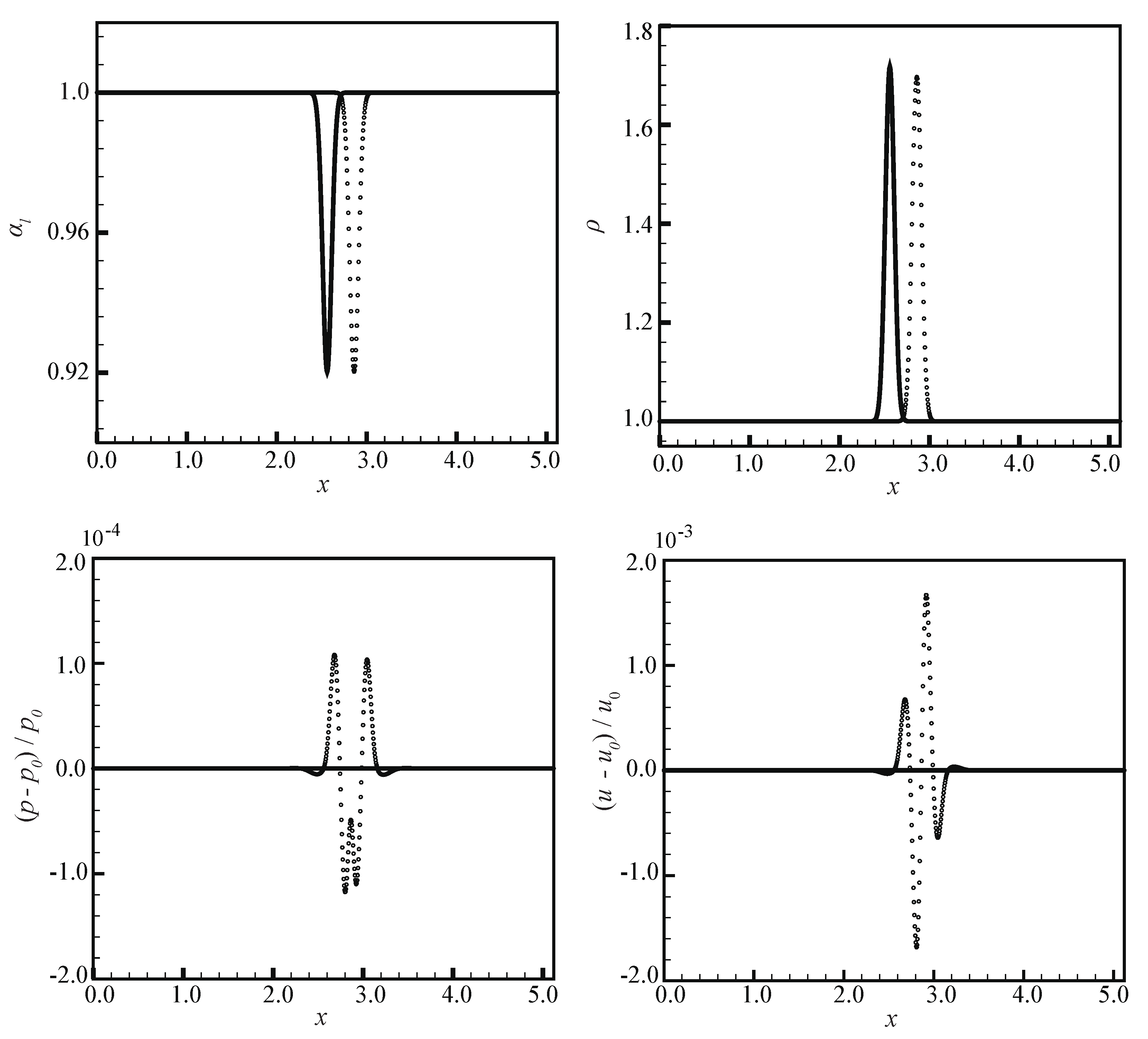
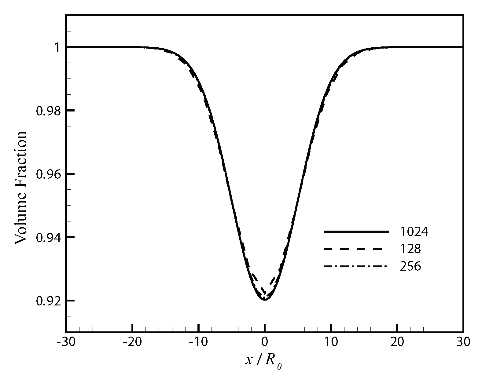
4.2. 1D Bubble Advection

When a gas bubble streams with the same speed as the carrier fluid under no-slip motion, the exact solution to this problem is the advection of the volume fraction and mixture density under a constant speed. The numerical model should also preserve the constant pressure and velocity profile along the streamline well. In the dispersed Lagrangian model, the advected interface leads an inconsistency between the volume fraction α g and the mixture pressure p because the volume fraction is evaluated directly from the bubbles’ sizes and locations. Indeed, the numerical oscillation induced from this inconsistency cannot be removed completely.
We consider one gas bubble inside another phase with the following initial states:
ρ , u 0 , p 0 , γ E T = 1.0 , 0.1 , 1.0 , 1.4 T ρ , u 0 , p 0 , γ L T = 10.0 , 0.1 , 1.0 , 1.6 T ,
where the subscripts `E’ and `L’ denote the Eulerian phase and Lagrangian phase, respectively. Dimensional unites are given by using 1 atm and 0.1 mm. The length of the computational domain is 5.12, with a finest resolution of 1024. A Lagrangian bubble with initial diameter of 0.02 is placed at the domain center. The kernel width is initialized as σ = 0.03 . Figure 4 gives the volume fraction α l , mixture density ρ , pressure difference ( p p 0 ) / p 0 , and velocity difference ( u u 0 ) / u 0 at t = 0 and t = 3 . A numerical peak emerges after the first time-step and propagates afterwards. The normalized magnitude of the pressure and velocity oscillation has been limited to the order of 10 4 and 10 3 , respectively, which is acceptable for later simulations.

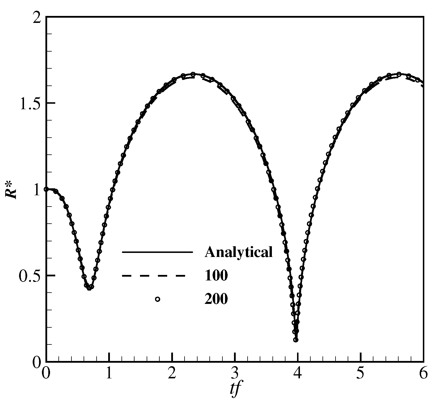
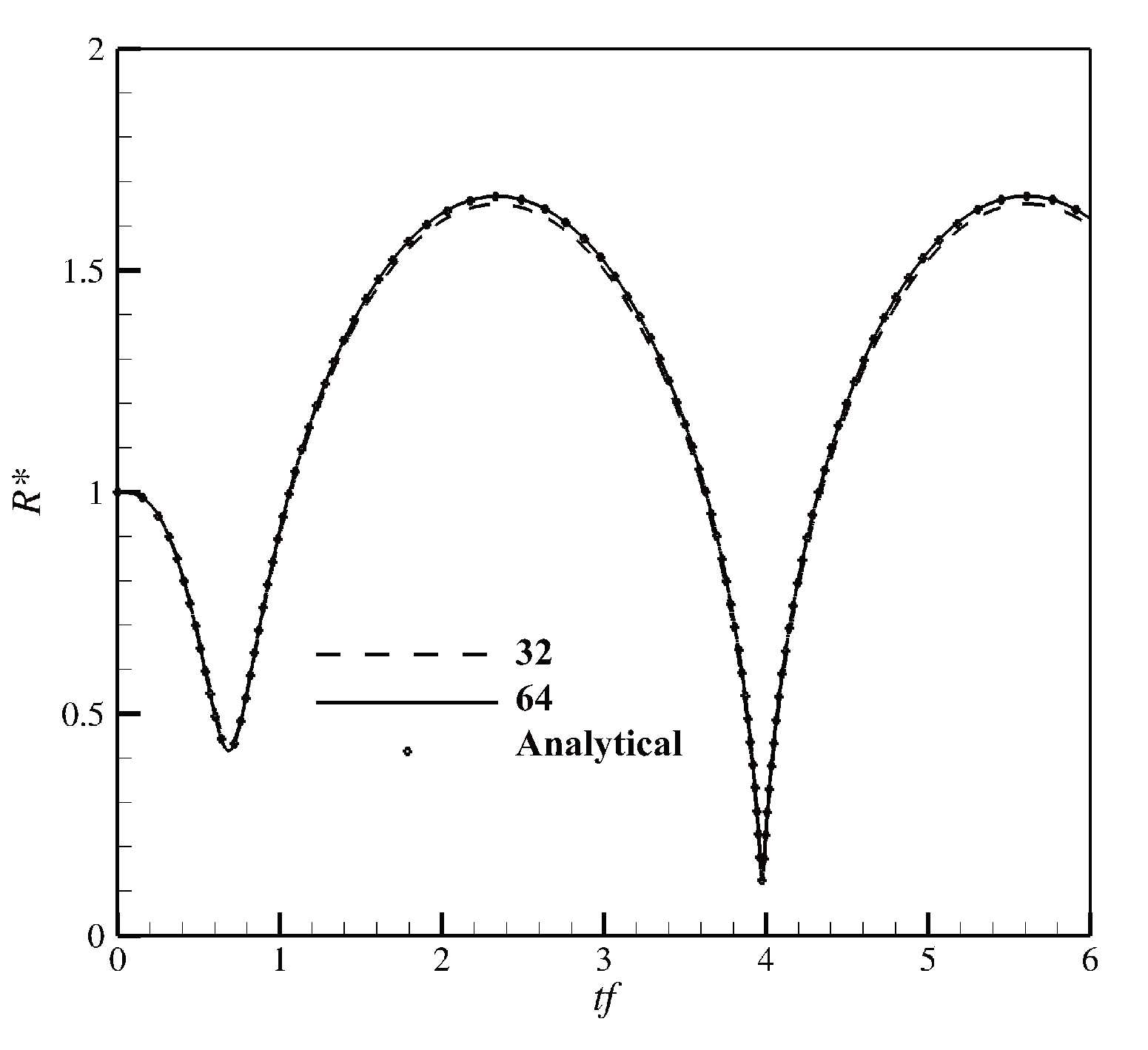
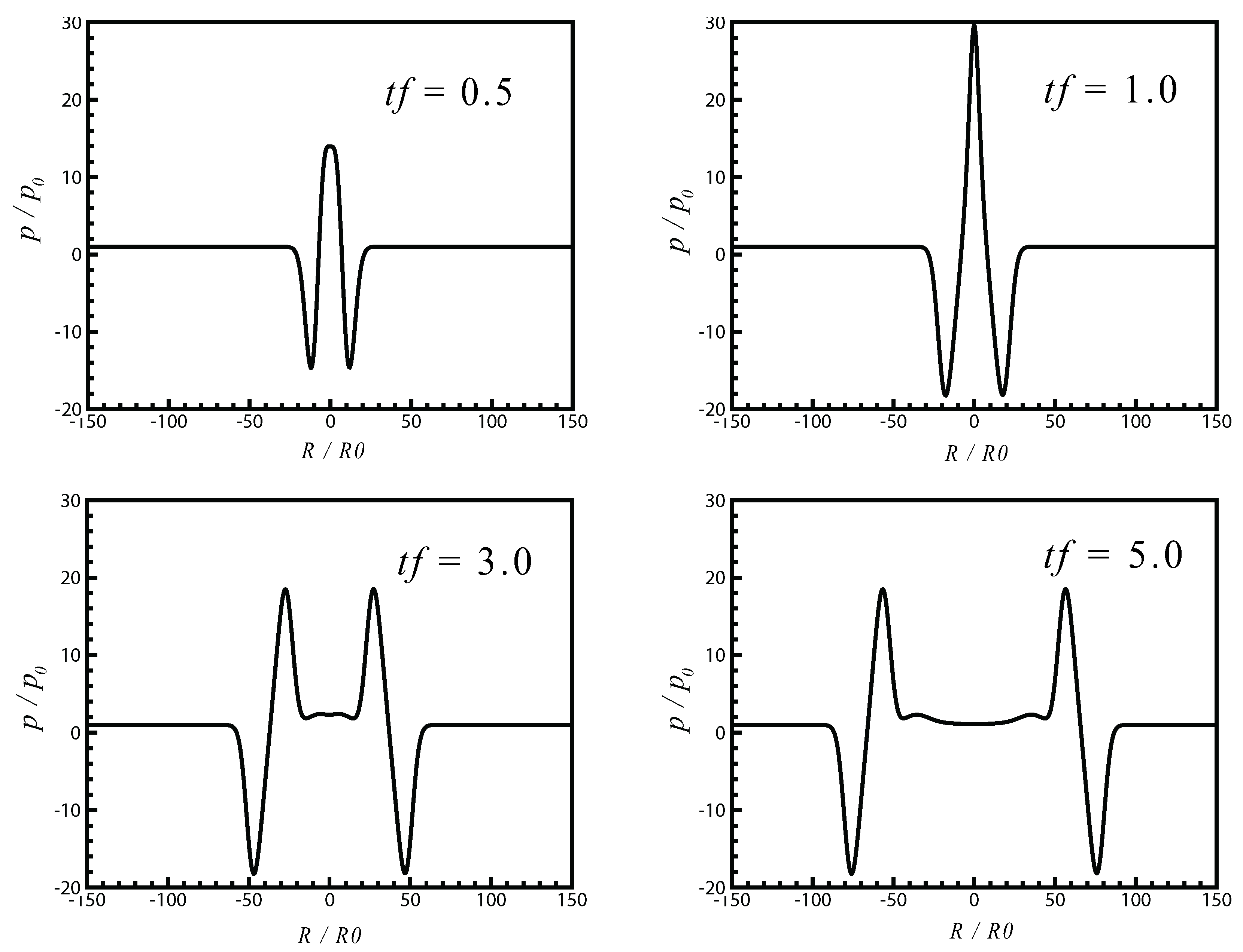
4.3. Single Bubble Oscillating

In this part, we consider a single gas bubble oscillating inside water. The Rayleigh collapse is a typical transient behavior when there is an over-pressure from the surrounding fluid. The Rayleigh time, the approximated characteristic bubble collapse time, for a single vapor bubble, gives
t Rayleigh = 0.915 R 0 ρ l p p v .
The bubble oscillates actively as R = R 0 1 ε sin 2 π ω t , where ε is the perturbation magnitude, and ω is the frequency. We set R 0 = 100 μ m , ε = 0.1 , and ω = 100 kHz . The 1D dimension length is L = 300 R 0 . The bubble is initially located at the center of the domain. The width of the support in the Gaussian kernel is initialized as σ = 6.0 R 0 . Figure 5 presents the volume fraction α l along the radial axial under three different resolutions, i.e., 128, 256, and 1024. The resolution of 1024 is used for the further simulations.
The bubble oscillates actively only for a half period 0.5 t f ; afterwards, the volume of the bubble returns to its initial radius and remains still. In Figure 6, the pressure wave along the radius axis at t * = t f = 0.5 , 1.0 , 3.0 , and 5.0 are given. The bulk fluid is expanded, at first, and then compressed due to the variation of the bubble. As a result, a first-negative and second-positive pressure wave propagating along the radius axis presents. Figure 7 gives the pressure waves along the radius axis at t * = t f = 0.5 , 1.0 , 3.0 , and 5.0 of the second case, in which the bubble oscillates continuously without pause. It can be observed that the amplitude and frequency of the continuous pressure waves induced by the bubble oscillation are also well resolved.

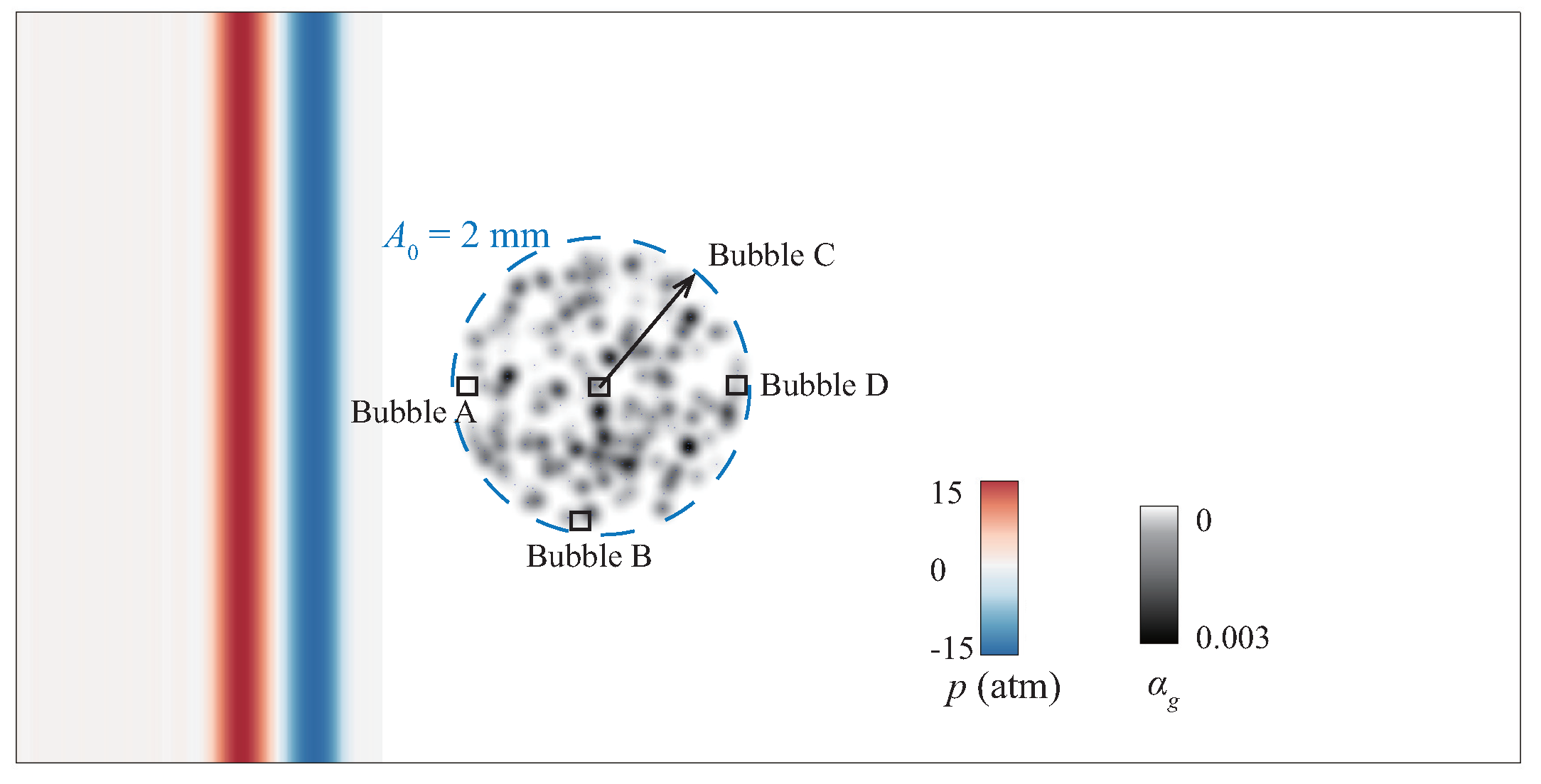
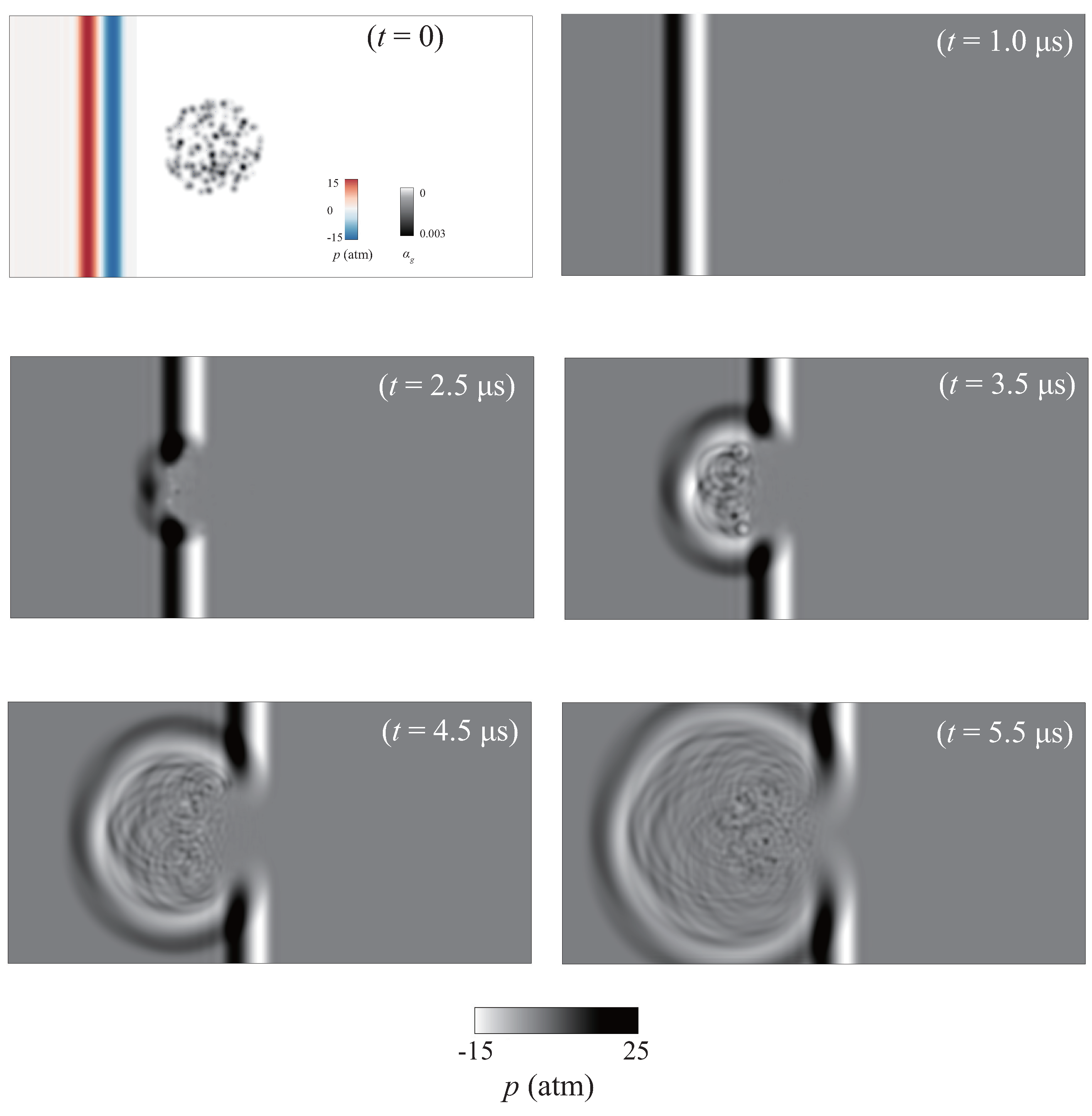
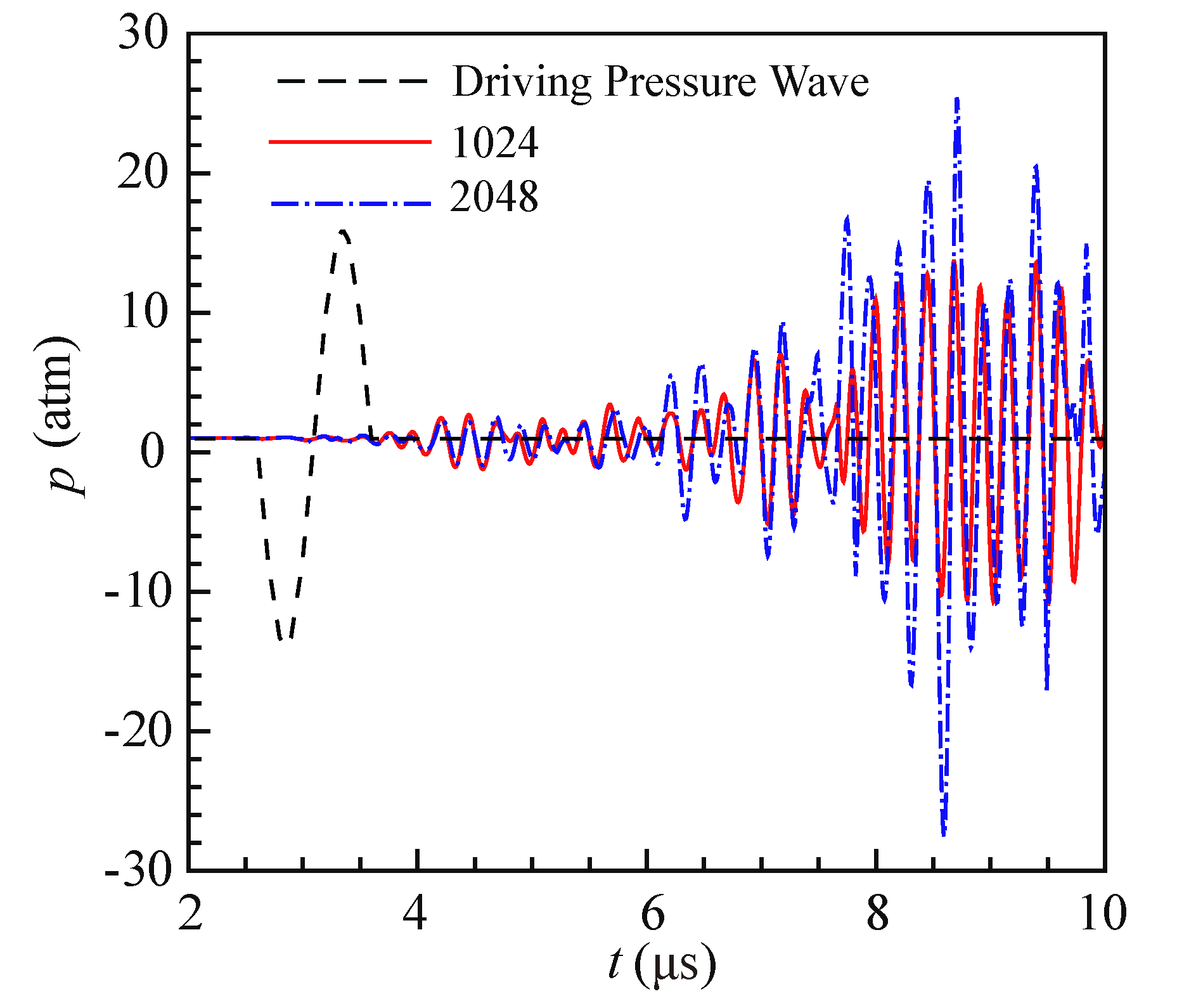
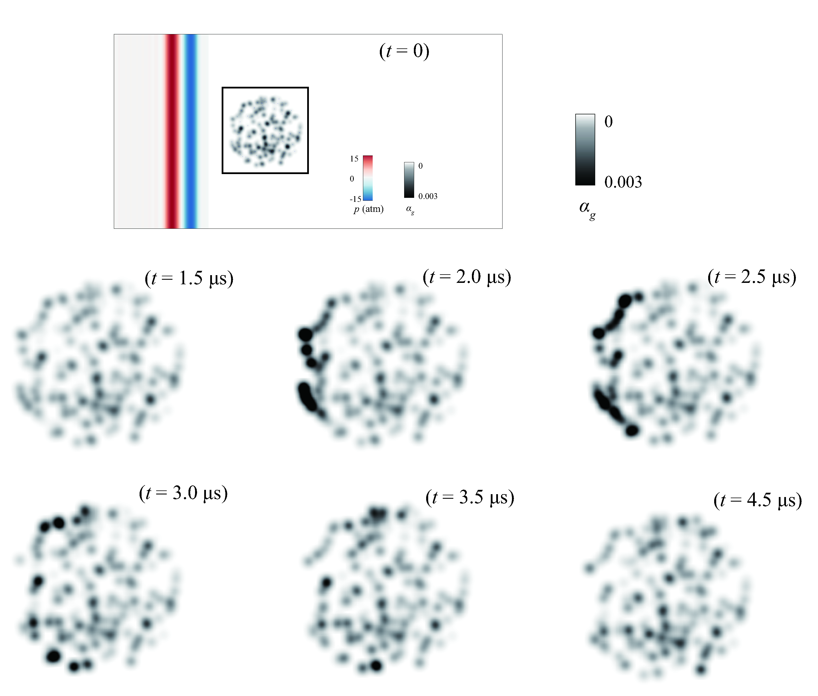
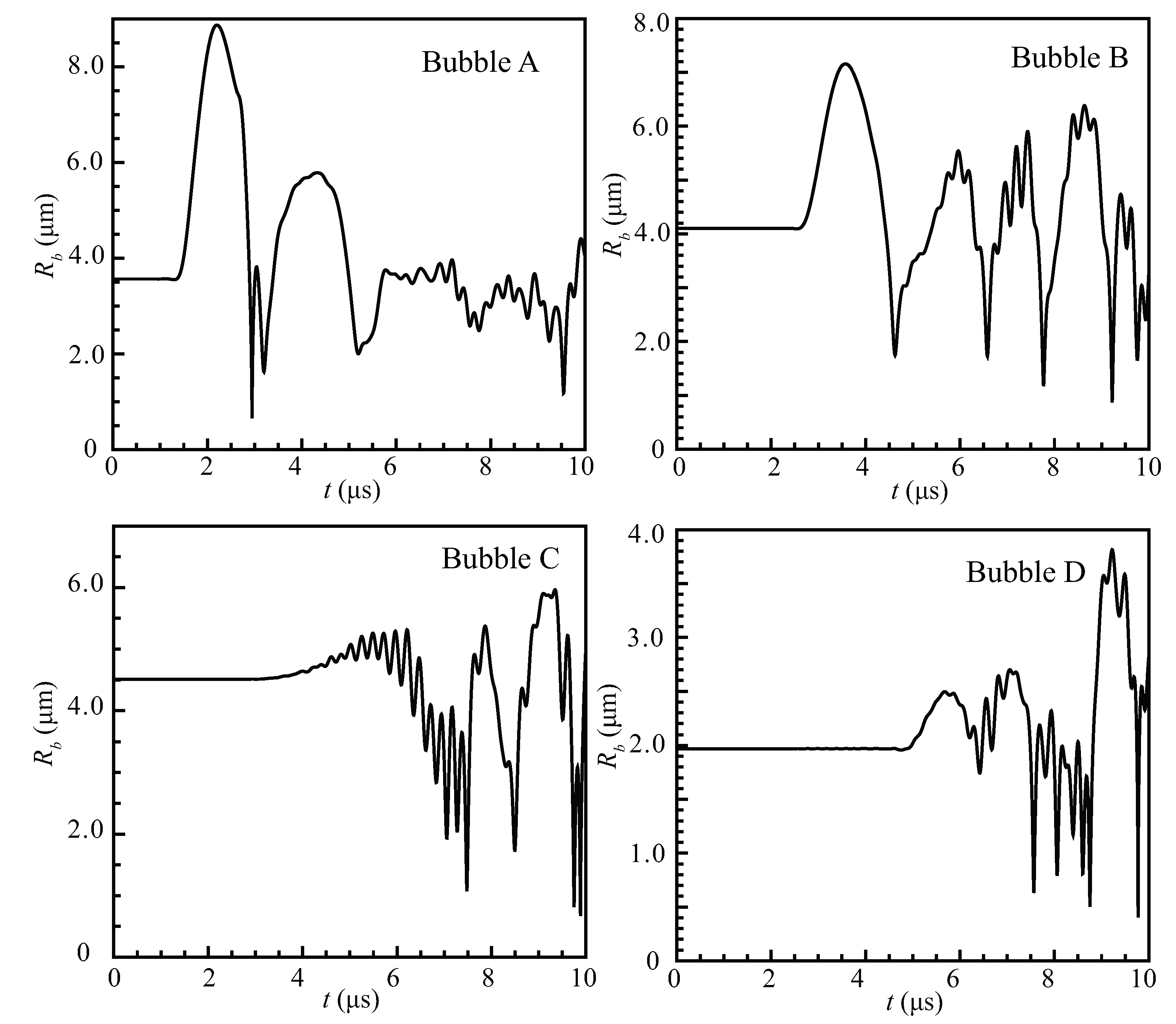
5. Application of a Bubble Cloud Interacting with Pressure Wave

The interaction between a cavitation bubble cloud and a pressure wave is important in many biomedical and chemical applications [40]. To better understand the transformation of the pressure wave when it passes through a bubble cloud, and to analyze the acoustic pressure oscillation induced by the bubble cluster, a 2D cylindrical bubble cloud interacting with a sinusoidal pressure pulse in the fluid is simulated. According to the research in Reference [20], the bulk fluid has low nuclei concentration with the gas volume fraction in the order of 10 5 and 10 4 . Under the lower gas volume fraction, the shape of the pressure wave is only slightly disturbed by the dispersed bubbles [41]. In the present work, the average gas volume fraction is larger, which is in the order of 10 3 .
Figure 8 shows the bubble cloud with a radius of A 0 = 2 mm containing 200 gas bubbles with a random radius distribution between 1 μ m and 5 μ m . The scattered black tiny points represent the bubbles, and the gas fraction α g , which ranges from 0.0 to 0.003 , colored by a gray scale contour, is used to visualize the bubbles distribution. The sinusoidal pressure wave moving from left to right is initialized by using p = p 0 + Δ p sin 2 π x x 0 λ , with a wave length of λ = 0.5 A 0 and amplitude of Δ p = 15 atm and the pressure at infinity p 0 = 1.0 atm . The negative pressure reaches the bubble cloud first, inducing the bubbles to expand. The initial velocity field is set to zero. The computational domain is 2 L × L (L = 10.24 mm), and the finest resolution is 2048 × 1024 . The kernel width for each gas bubble is initialized as σ = 3.0 dx, with dx denoting the finest grid size. Four bubbles, i.e., Bubble A (on the left side), Bubble B (on the bottom), Bubble C (at bubble cloud center), and Bubble D (on the right side), are marked. They are used to analyze the influence of the pressure wave on the bubbles at different locations in the cloud.
At t = 0, the center of the bubble cloud is at ( 0.5 L , 0.78 L ), and the center of the pressure wave is at x 0 = 0.34 L . Then, the pressure wave propagates from left to right and interacts with the bubble cluster. The pressure fields at 1.0 μ s , 2.5 μ s , 3.5 μ s , 4.5 μ s , and 5.5 μ s are shown in Figure 9. It can be observed that the pressure wave reaches the bubble cluster boundary and is reflected by the cloud boundary. When the fluid has a low gas volume fraction, the shape of the pressure wave is almost unaffected [20]. In our results, the pressure wave is partially reflected, and the rest of the wave travels through the cluster. The bubbles vibrate when the pressure arrives, while remaining in equilibrium with the bulk fluid before the pressure wave.
As shown in Figure 9, the pressure pulse inside the bulk fluid induces the bubbles’ vibration. In turn, the vibration of the gas bubbles induces the pressure disturbance in the bulk fluid. The evolution of the pressure p at the cloud’s center is reported in Figure 10. This results correspond to two different resolutions on x-axis. The driving pressure wave propagation in the liquid without the bubble cloud is also plotted. With a higher resolution of 2048 in x-axis, the amplitude of the pressure wave is increased. Note that the frequency of the pressure wave has already been resolved well with a resolution of 1024. Due to bubbles’ oscillation and bubble-bubble interactions, the pressure at the cloud center can reach an amplitude of 30 atm.
Meanwhile, in Figure 11, the volume fraction α g at 1.5 μ s , 2.0 μ s , 2.5 μ s , 3.0 μ s , 3.5 μ s , and 4.5 μ s is given. Generally, a larger gas volume fraction would be achieved when negative pressure approaches the bubbles as the bubbles expand. Instead, overpressurization compresses the bubbles, indicating a smaller value of α g . As the pressure wave is partially reflected at the cluster’s boundary, there is no major change in the volume fraction at the cloud’s center. To better understand the influence of the pressure wave on α g , the time evolution of radii for Bubble A–D is recorded in Figure 12. From Figure 12, it can be observed that the bubbles’ radii are constant before the arrival of the pressure wave, which means the bubbles are in equilibrium with the carrier fluid. The negative pressure first reaches Bubble A, inducing its violent expansion. This corresponds well with the larger volume fraction field at t = 2.0 μ s in Figure 11. The positive pressure wave follows and condenses Bubble A, which makes the bubble unstable and oscillates actively. Similarly, Bubble B expands, at first, then shrinks, and finishes by actively oscillating. However, for Bubble C (at the cloud’s center) and D (on the right), no obvious expansion presents when the pressure wave arrives. The difference of the bubble radius history is induced by the fact that the pressure wave is damped when it propagates to Bubble C and even becomes weak at Bubble D due to the reflection and absorbing during the interaction. This phenomenon corresponds well with the volume fraction field at t = 3.0 μ s , 3.5 μ s , and 4.5 μ s in Figure 11. As also shown in Figure 9, the pressure wave is reflected at the interface and absorbed, and only a small amount of the pressure successfully passes the bubble cloud. In the end, all four bubbles actively oscillate as a result of the pressure wave, until they return to a state of equilibrium with the carrier fluid.

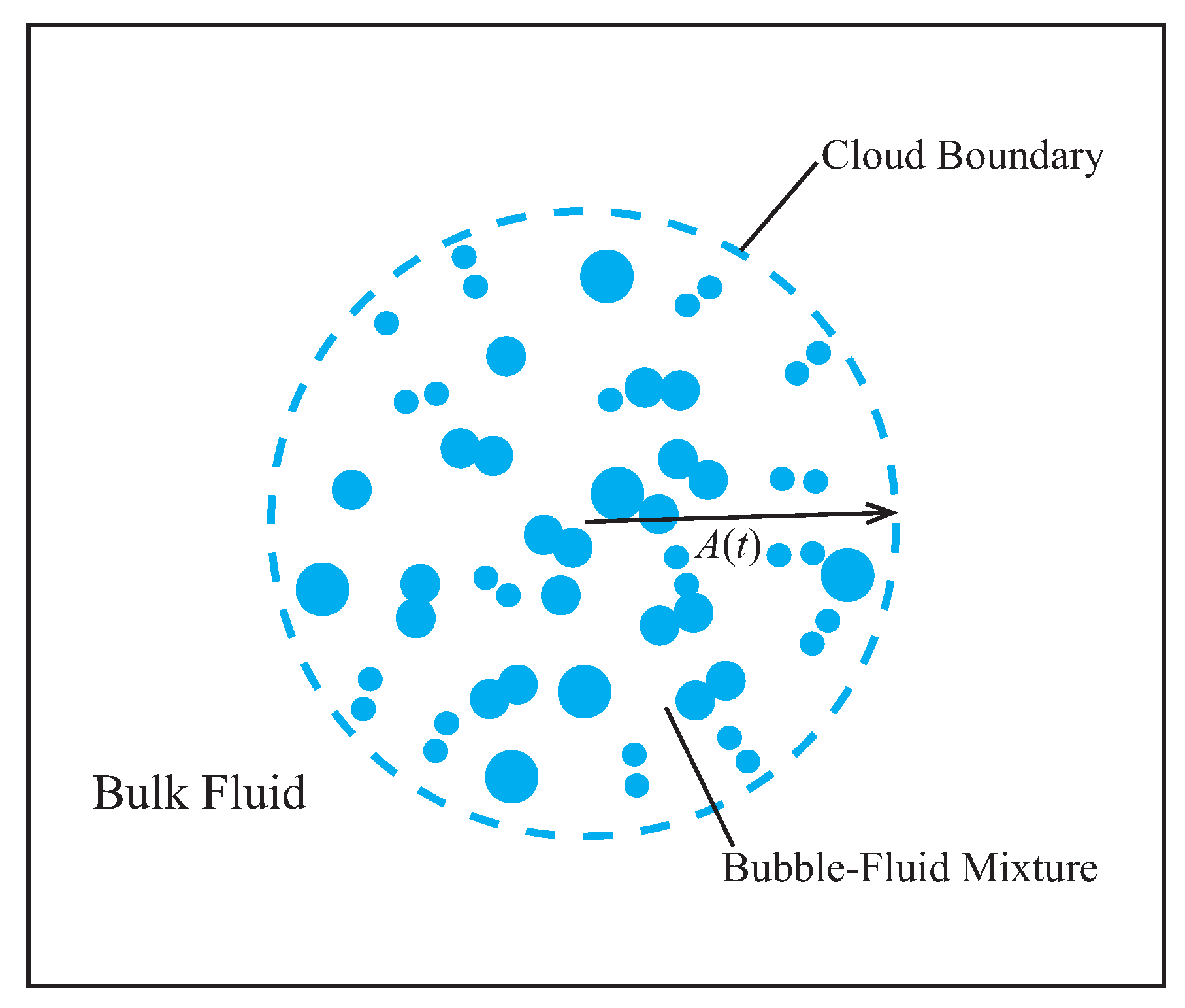
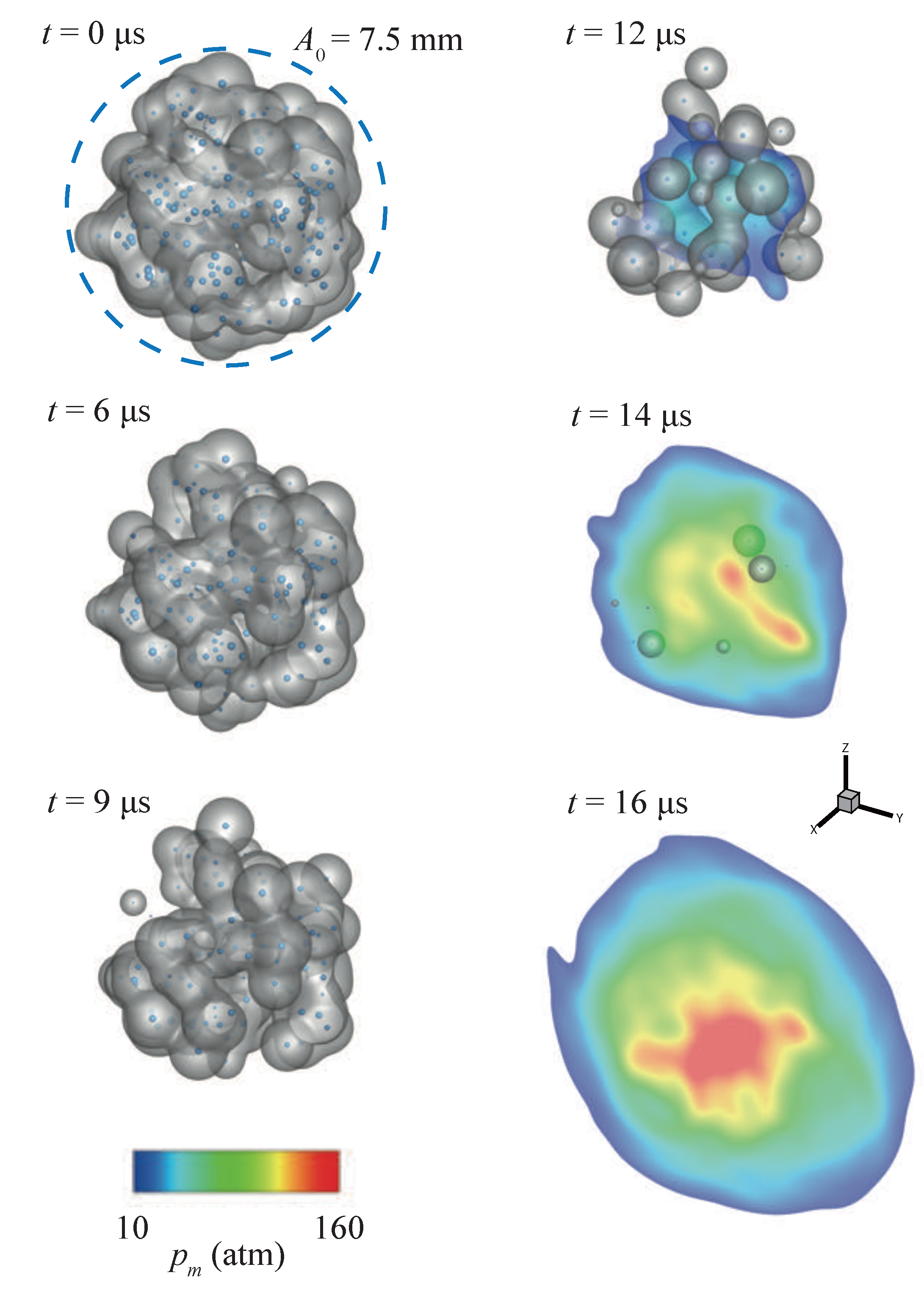
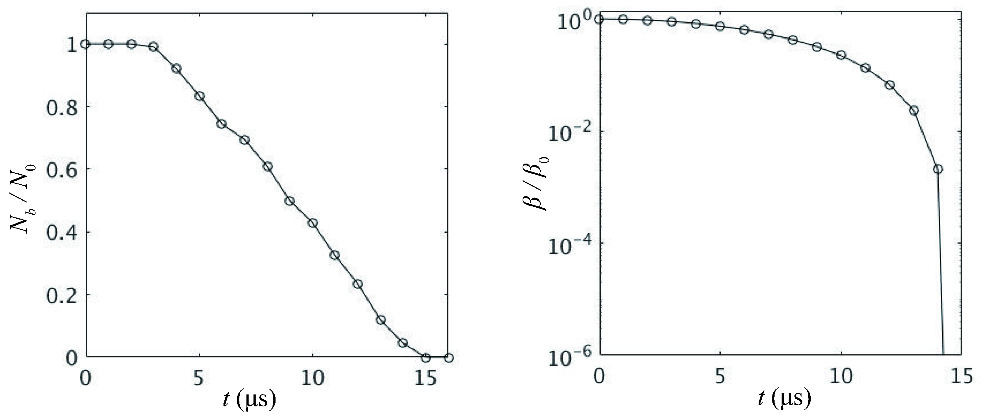
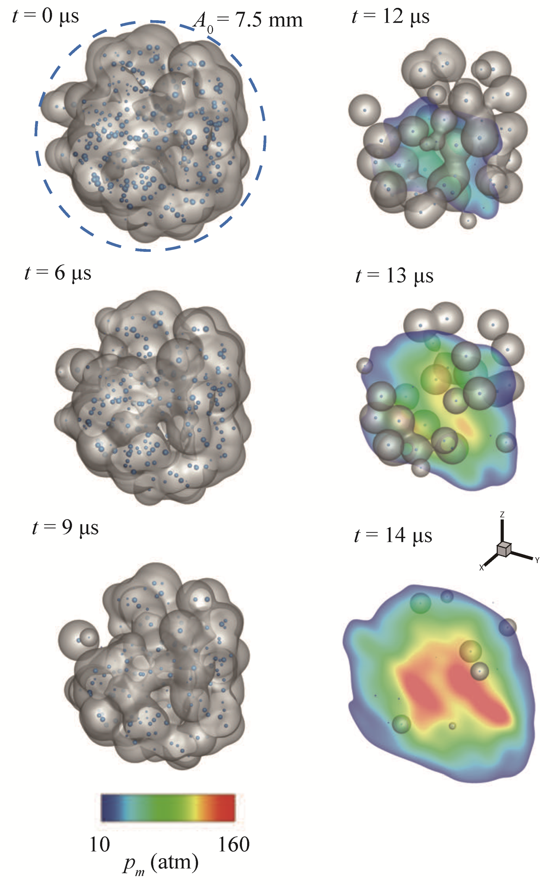
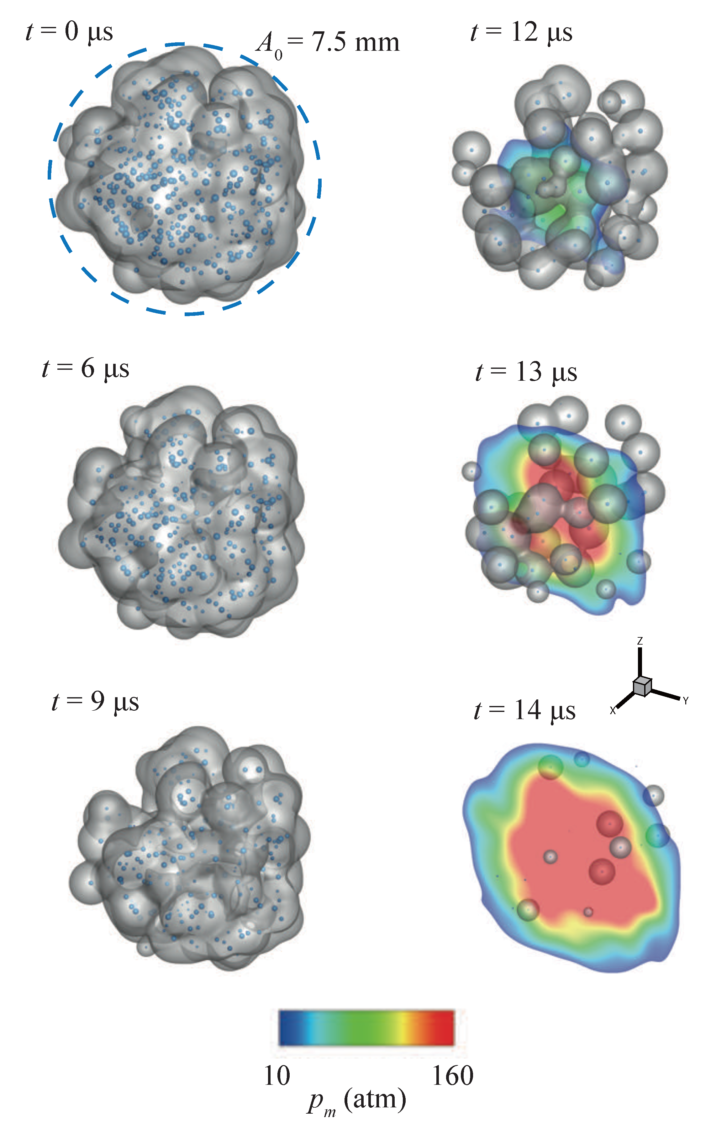
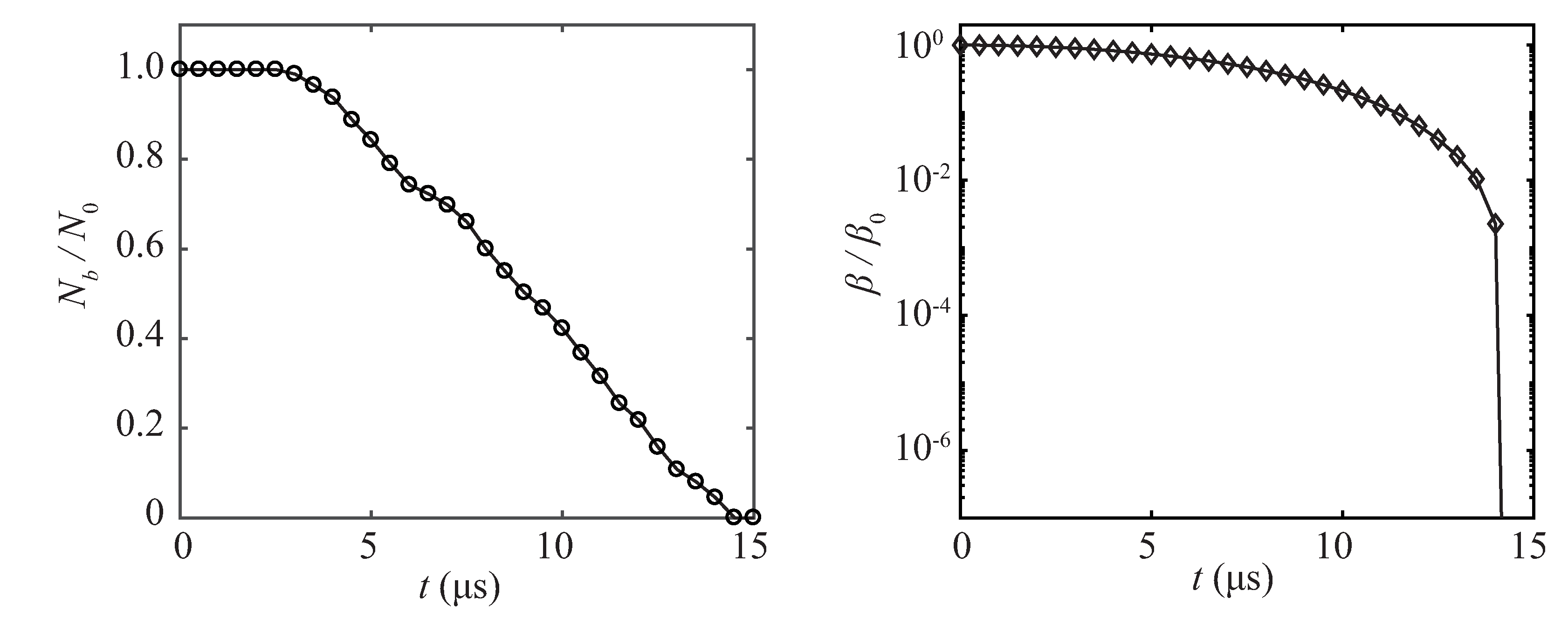
6. Rayleigh Collapse of a Bubble Cloud

Collapsing bubbles are essential in the applications of underwater explosions, ultrasonic cleaning, and non-invasive biomedical processes. However, a complex pressure field presents in the whole process, involving shock waves and acoustic pressure disturbances, which is hardly detected and distinguished experimentally. In addition, the detailed collapse dynamics of bubble clusters has been poorly investigated in experiments as the length and time scale during the collapse and bubble oscillation could hardly be detected due to measurement limitations. In this section, we perform a 3D simulation for the Rayleigh collapse of a cavitation vapor bubble cloud and study the extreme pressure induced by the violent collapse of bubbles, as well as the size distribution of bubbles during the collapse, in detail.

6.1. Rayleigh Collapse

The schematic of the initial set-up is shown in Figure 13. First, a spherical bubble cluster with N 0 = 200 spherical bubbles is placed into still water, the radii of which are initially randomly distributed between 100 μ m and 500 μ m. The radius of the bubble cluster is A 0 = 7.5 mm, with averaged bubble radius 308 μ m. The 3D domain size is 25.6 mm × 25.6 mm × 25.6 mm, and the resolution at the finest level is set as [ 256 × 256 × 256 ] . The center of the bubble cluster coincides with the center of the computational domain. All boundary conditions are out-flow conditions. The velocity field is initialized as zero, and the temperature remains constant at 293 K. The viscosity and the non-condensible gas inside the bubbles are neglected. All the bubbles are vapor bubbles, and the vapor pressure remains constant with p v = 2430 pa. The initial bulk fluid over-pressure is p = 10.0 atm. The initial strong over-pressure induces the violent collapse of the cloud. To save computation efforts, bubbles with extremely small volume are labeled as “inactive” to signify their collapse, and the Lagrangian computation of the inactive bubbles will be terminated. Thus, in the present collapse simulation, the cloud rebound will not be considered. The collapse time here refers to the time at which the bubble cloud meets the first collapse point. For the coupling scheme, the width of the Gaussian kernel function is initialized as σ 0 = 6.0 d x .

6.2. Results and Discussion

Figure 14 gives six snapshots of the collapsing process of a bubble cloud. The iso-surface of volume fraction α g = 0.002 is visualized with gray color to represent the vapor bubble distributions. In addition, the spherical vapor bubbles, indicating the location and volume, are also presented with blue color. The non-symmetrical collapse process happens from outside to inside. At the beginning of the process, until around t = 9 μ s, the cloud collapses slowly. After that point, the rate of the collapse increases considerably, and the bubble cloud collapses violently between 14 μ s and 16 μ s. The obtained collapse agrees qualitatively well with the first collapse of the simulation result in Reference [18].
During the collapse, extremely high pressures are generated from the center of the bubble cloud. In Figure 14, the slices of the higher pressure region, where the pressure is greater than 10 atm, are presented at each time instant. The higher pressure increases over time. At the end of the collapse process, the extreme pressure reaches its maximum value around 174 atm when the collapse rate reaches its maximum value. In Figure 15, revolutions of the dimensionless active bubble number N b / N 0 and the dimensionless averaged gas fraction β / β 0 ( β = Σ V c α g / V c ) are reported. The vapor clouds collapse completely at about t = 14.5 μ s.
To analyze the influence of the bubble initial number N 0 on the cloud’s collapse time, we simulate N 0 = 300 and 400 under the same initial condition as above. Figure 16 and Figure 17 provide snapshots of the collapse process at t = 0 μ s, 6 μ s, 9 μ s, 12 μ s, 13 μ s, and 14 μ s. In Figure 18, the time history of N b / N 0 ( N 0 = 400) and β / β 0 are given. We can observe that, similar to N 0 = 200 in Figure 15, the collapse time of the bubble cloud with N 0 = 300 or N 0 = 400 is also around 14.5 μ s. However, the larger bubble number leads to greater violent pressure at the cloud’s center. The maximum pressure for N 0 = 300 is roughly 226 MPa, while, for N 0 = 400, the maximum pressure is about 313 MPa.
For the case of the bubble cloud with N 0 = 400, the distribution of bubble radii during the collapse is analyzed according to their sizes. Figure 19 shows the bubble size density distribution at t = 0 μ s, 6 μ s, 9 μ s, 12 μ s, 13 μ s, and 14 μ s. The first bar on the left side indicates the density of the collapsed (inactive) vapor bubbles. From Figure 19, we can observe that the vapor bubbles become compressed all together because of the higher environmental pressure. As given in Equation (22), with a bubble radius increases, its collapse time t Rayleigh also increases. For a bubble cloud, we find that there are two factors affecting the final collapse time, i.e., the bubble size distribution and the initial overpressurization. In the three above conditions of different initial bubble numbers, bubbles in the cloud follow the same initial size distribution, which means the average bubble radius remains unaltered. When the bubble radius distribution remains unchanged, the number of bubbles inside the cloud has no significant influence on the time instant when the cloud finally collapses, except a larger bubble number increasing the averaged vapor volume fraction β = Σ V c α g / V c . However, the larger bubble number induces greater pressure at the cloud’s center because of a larger vapor void.

7. Concluding Remarks

In this paper, an LE two-way coupling model is developed based on a multi-resolution Eulerian solver. To close the system of governing equations, an isobaric pressure closure is applied. The gas fraction is modeled as a formulation of the sizes and locations of the gas bubbles. Benchmark cases are used to validate the present method in both 1D and 3D contexts. The simulation of a cylindrical bubble cloud interacting with a pressure wave is carried out as one application. The results reveal that the shape of the pressure pulse in the fluid significantly changes after passing through the bubble cloud due to the reflection at the cloud’s boundary and at the sub-grid interfaces when the gas void fraction is in the scale of 10 3 . In the 3D simulation of Rayleigh collapse of a bubble cloud, it is observed that the number of bubbles inside the cloud has no notable influence on the cloud’s final collapse time if the bubble size distribution remains the same. However, the larger number of bubbles leads the higher of averaged vapor volume fraction, thus inducing more violent, higher pressures.

Author Contributions

X.L. and Y.Z.: Investigation, Methodology, Visualization, Validation, Formal analysis, Writing—original draft, Writing—review & editing; C.Z.: Investigation, Writing—review & editing; X.H. and N.A.A.: Investigation, Supervision, Writing—review & editing. All authors have read and agreed to the published version of the manuscript.

Funding

X. Lyu acknowledges the scholarship from the China Scholarship Council under No.201406120010. Y. Zhu acknowledges the National Natural Science Foundation of China (NSFC) (Grant No.: 91952110).

Institutional Review Board Statement

Not applicable.

Informed Consent Statement

Not applicable.

Data Availability Statement

Data can be obtained by contacting the corresponding author.

Conflicts of Interest

The authors declare no conflict of interest.

References

  1. Darmana, D.; Deen, N.G.; Kuipers, J.A.M. Detailed modeling of hydrodynamics, mass transfer and chemical reactions in a bubble column using a discrete bubble model. Chem. Eng. Sci. 2005, 60, 3383–3404. [Google Scholar] [CrossRef] [Green Version]
  2. Singh, R.N.; Sharma, S. Development of suitable photobioreactor for algae production—A review. Renew. Sustain. Energy Rev. 2012, 16, 2347–2353. [Google Scholar] [CrossRef]
  3. Coussios, C.C.; Roy, R.A. Applications of acoustics and cavitation to noninvasive therapy and drug delivery. Annu. Rev. Fluid Mech. 2008, 40, 395–420. [Google Scholar] [CrossRef]
  4. Vlaisavljevich, E.; Lin, K.W.; Warnez, M.T.; Singh, R.; Mancia, L.; Putnam, A.J.; Johnsen, E.; Cain, C.; Xu, Z. Effects of tissue stiffness, ultrasound frequency, and pressure on histotripsy-induced cavitation bubble behavior. Phys. Med. Biol. 2015, 60, 2271. [Google Scholar] [CrossRef] [PubMed] [Green Version]
  5. Ohl, C.D.; Arora, M.; Dijkink, R.; Janve, V.; Lohse, D. Surface cleaning from laser-induced cavitation bubbles. Appl. Phys. Lett. 2006, 89, 074102. [Google Scholar] [CrossRef]
  6. Balachandar, S.; Eaton, J.K. Turbulent dispersed multiphase flow. Annu. Rev. Fluid Mech. 2010, 42, 111–133. [Google Scholar] [CrossRef]
  7. Matsumoto, Y.; Allen, J.S.; Yoshizawa, S.; Ikeda, T.; Kaneko, Y. Medical ultrasound with microbubbles. Exp. Therm. Fluid Sci. 2005, 29, 255–265. [Google Scholar] [CrossRef]
  8. Lauer, E.; Hu, X.; Hickel, S.; Adams, N.A. Numerical investigation of collapsing cavity arrays. Phys. Fluids 2012, 24, 052104. [Google Scholar] [CrossRef]
  9. Lauer, E.; Hu, X.Y.; Hickel, S.; Adams, N.A. Numerical modelling and investigation of symmetric and asymmetric cavitation bubble dynamics. Comput. Fluids 2012, 69, 1–19. [Google Scholar] [CrossRef]
  10. Tiwari, A.; Pantano, C.; Freund, J.B. Growth-and-collapse dynamics of small bubble clusters near a wall. J. Fluid Mech. 2015, 775, 1–23. [Google Scholar] [CrossRef]
  11. Stride, E.; Coussios, C. Cavitation and contrast: The use of bubbles in ultrasound imaging and therapy. Proc. Inst. Mech. Eng. Part H J. Eng. Med. 2010, 224, 171–191. [Google Scholar] [CrossRef]
  12. Hauptmann, M.; Struyf, H.; De Gendt, S.; Glorieux, C.; Brems, S. Evaluation and interpretation of bubble size distributions in pulsed megasonic fields. J. Appl. Phys. 2013, 113, 184902. [Google Scholar] [CrossRef]
  13. Iida, Y.; Ashokkumar, M.; Tuziuti, T.; Kozuka, T.; Yasui, K.; Towata, A.; Lee, J. Bubble population phenomena in sonochemical reactor: I Estimation of bubble size distribution and its number density with pulsed sonication–Laser diffraction method. Ultrason. Sonochem. 2010, 17, 473–479. [Google Scholar] [CrossRef] [PubMed]
  14. Maeda, K. Simulation, Experiments, and Modeling of Cloud Cavitation with Application to Burst Wave Lithotripsy. Ph.D. Thesis, California Institute of Technology, Pasadena, CA, USA, 2018. [Google Scholar]
  15. Ando, K.; Colonius, T.; Brennen, C.E. Numerical simulation of shock propagation in a polydisperse bubbly liquid. Int. J. Multiph. Flow 2011, 37, 596–608. [Google Scholar] [CrossRef]
  16. Delale, C.F.; Nas, S.; Tryggvason, G. Direct numerical simulations of shock propagation in bubbly liquids. Phys. Fluids 2005, 17, 121705. [Google Scholar] [CrossRef]
  17. Calzavarini, E.; Kerscher, M.; Lohse, D.; Toschi, F. Dimensionality and morphology of particle and bubble clusters in turbulent flow. J. Fluid Mech. 2008, 607, 13–24. [Google Scholar] [CrossRef] [Green Version]
  18. Egerer, C.P.; Schmidt, S.J.; Hickel, S.; Adams, N.A. Efficient implicit LES method for the simulation of turbulent cavitating flows. J. Comput. Phys. 2016, 316, 453–469. [Google Scholar] [CrossRef]
  19. Lauterborn, W.; Kurz, T. Physics of bubble oscillations. Rep. Prog. Phys. 2010, 73, 106501. [Google Scholar] [CrossRef]
  20. Fuster, D.; Colonius, T. Modelling bubble clusters in compressible liquids. J. Fluid Mech. 2011, 688, 352–389. [Google Scholar] [CrossRef] [Green Version]
  21. Allaire, G.; Clerc, S.; Kokh, S. A five-equation model for the simulation of interfaces between compressible fluids. J. Comput. Phys. 2002, 181, 577–616. [Google Scholar] [CrossRef] [Green Version]
  22. Gorokhovski, M.; Herrmann, M. Modeling primary atomization. Annu. Rev. Fluid Mech. 2008, 40, 343–366. [Google Scholar] [CrossRef]
  23. Ma, J.; Hsiao, C.T.; Chahine, G.L. Numerical study of acoustically driven bubble cloud dynamics near a rigid wall. Ultrason. Sonochem. 2018, 40, 944–954. [Google Scholar] [CrossRef]
  24. Maeda, K.; Colonius, T. Bubble cloud dynamics in an ultrasound field. J. Fluid Mech. 2019, 862, 1105–1134. [Google Scholar] [CrossRef] [PubMed] [Green Version]
  25. Lyu, X.; Pan, S.; Hu, X.; Adams, N.A. Numerical investigation of homogeneous cavitation nucleation in a microchannel. Phys. Rev. Fluids 2018, 3, 064303. [Google Scholar] [CrossRef]
  26. Darmana, D.; Deen, N.G.; Kuipers, J. Parallelization of an Euler–Lagrange model using mixed domain decomposition and a mirror domain technique: Application to dispersed gas–liquid two-phase flow. J. Comput. Phys. 2006, 220, 216–248. [Google Scholar] [CrossRef]
  27. Rayleigh, L. VIII. On the pressure developed in a liquid during the collapse of a spherical cavity. Lond. Edinb. Dublin Philos. Mag. J. Sci. 1917, 34, 94–98. [Google Scholar] [CrossRef]
  28. Plesset, M.S. The dynamics of cavitation bubbles. J. Appl. Mech. 1949, 16, 277–282. [Google Scholar] [CrossRef]
  29. Shams, E.; Finn, J.; Apte, S.V. A numerical scheme for Euler–Lagrange simulation of bubbly flows in complex systems. Int. J. Numer. Methods Fluids 2011, 67, 1865–1898. [Google Scholar] [CrossRef]
  30. Abgrall, R. How to prevent pressure oscillations in multicomponent flow calculations: A quasi conservative approach. J. Comput. Phys. 1996, 125, 150–160. [Google Scholar] [CrossRef] [Green Version]
  31. Saurel, R.; Abgrall, R. A multiphase Godunov method for compressible multifluid and multiphase flows. J. Comput. Phys. 1999, 150, 425–467. [Google Scholar] [CrossRef]
  32. Hu, X.; Adams, N.; Herrmann, M.; Iaccarino, G. Multi-scale modeling of compressible multi-fluid flows with conservative interface method. In Proceedings of the Summer Program; Center for Turbulence Research, Stanford University: Stanford, CA, USA, 2010; Volume 301. [Google Scholar]
  33. Han, L.H.; Hu, X.Y.; Adams, N.A. Adaptive multi-resolution method for compressible multi-phase flows with sharp interface model and pyramid data structure. J. Comput. Phys. 2014, 262, 131–152. [Google Scholar] [CrossRef]
  34. Jiang, G.S.; Shu, C.W. Efficient Implementation of Weighted ENO Schemes. J. Comput. Phys. 1996, 126, 202–228. [Google Scholar] [CrossRef] [Green Version]
  35. Roe, P.L. Approximate Riemann solvers, parameter vectors, and difference schemes. J. Comput. Phys. 1981, 43, 357–372. [Google Scholar] [CrossRef]
  36. Johnsen, E.; Colonius, T. Implementation of WENO schemes in compressible multicomponent flow problems. J. Comput. Phys. 2006, 219, 715–732. [Google Scholar] [CrossRef]
  37. Alehossein, H.; Qin, Z. Numerical analysis of Rayleigh-Plesset equation for cavitating water jets. Int. J. Numer. Methods Eng. 2007, 72, 780–807. [Google Scholar] [CrossRef]
  38. Hu, X.Y.; Khoo, B.C.; Adams, N.A.; Huang, F.L. A conservative interface method for compressible flows. J. Comput. Phys. 2006, 219, 553–578. [Google Scholar] [CrossRef]
  39. Maeda, K.; Colonius, T. Eulerian-Lagrangian method for simulation of cloud cavitation. J. Comput. Phys. 2018, 371, 994–2017. [Google Scholar] [CrossRef] [PubMed] [Green Version]
  40. Ohl, S.W.; Klaseboer, E.; Khoo, B.C. Bubbles with shock waves and ultrasound: A review. Interface Focus 2015, 5, 20150019. [Google Scholar] [CrossRef] [PubMed]
  41. Arora, M.; Ohl, C.D.; Lohse, D. Effect of nuclei concentration on cavitation cluster dynamics. J. Acoust. Soc. Am. 2007, 121, 3432–3436. [Google Scholar] [CrossRef] [PubMed] [Green Version]
Figure 1. Schematic of three interface types with respect to the computational grid: the fully-resolved, under-resolved, and sub-grid dispersed interfaces.
Water 13 02684 g001
Figure 2. Isolated bubble: The time history of the bubble size R * = R b / R b 0 in 1D simulation. Results of grid resolutions of 100 ( d x = 4 R b 0 ) and 200 ( d x = 2 R b 0 ) are compared with the analytical solution.
Water 13 02684 g002
Figure 3. Isolated bubble: The time history of the bubble size R * = R b / R b 0 in 3D simulation.
Water 13 02684 g003
Figure 4. 1D bubble advection: The solid line represents the initial fluid condition, and ∘ represents the results when the Lagrangian bubble reaches x = 2.86 at t = 3.0 .
Water 13 02684 g004
Figure 5. Single bubble oscillating: Volume fraction α l along the bubble radius for different resolutions.
Water 13 02684 g005
Figure 6. Single bubble oscillating: Pressure wave propagation induced from an oscillating gas bubble at t * = t f = 0.0 , 1.0 , 3.0 , and 5.0 .
Water 13 02684 g006
Figure 7. Single bubble oscillating: Pressure wave propagation induced from a continuous oscillating gas bubble at t * = t f = 0.0 , 1.0 , 3.0 , and 5.0 .
Water 13 02684 g007
Figure 8. Initial setup of the simulation of a bubble cloud interacting with pressure wave. The radius of the bubble cloud is A 0 = 2 mm , and it has 200 bubbles with random size distribution between 1 μ m and 5 μ m . The computation domain is 2 L × L (L = 10.24 mm). The distribution of the gas bubbles is visualized by both the volume fraction α g and the radius R b of Lagrangian spherical particles. Four bubbles (bubble A, B, C, and D) located at the four boxes’ centers are marked for future reference.
Water 13 02684 g008
Figure 9. The pressure field induced by the bubble cluster when the bubble cluster interacts with a sinusoidal pulse. The initial state and the pressure field at 1.0 μ s , 2.5 μ s , 3.5 μ s , 4.5 μ s , and 5.5 μ s are shown.
Water 13 02684 g009
Figure 10. The time history of pressure at the bubble cloud center without (the dashed line) and with bubble cloud for two different resolutions.
Water 13 02684 g010
Figure 11. The gas volume fraction α g when the bubble cluster interacts with a sinusoidal pulse at 1.5 μ s , 2.0 μ s , 2.5 μ s , 3.0 μ s , 3.5 μ s , and 4.5 μ s .
Water 13 02684 g011
Figure 12. The time history of bubble radius R b of Bubble A (on the left side), Bubble B (on the bottom), Bubble C (at bubble cloud center), and Bubble D (on the right side).
Water 13 02684 g012
Figure 13. Schematic of the set-up of the bubble cloud Rayleigh Collapse. A spherical bubble cloud with N 0 vapor bubbles is placed inside the bulk water. A ( t ) is the radius of the bubble cloud.
Water 13 02684 g013
Figure 14. The snapshots of the collapsing process of a bubble cloud with N 0 = 200 vapor bubbles (at t = 0 μ s, 6 μ s, 9 μ s, 12 μ s, 14 μ s, and 16 μ s). The distribution of the vapor bubbles is visualized both by the iso-surfaces of the volume fraction α g = 0.002 ( α l = 0.998 ) and the Lagrangian spherical particles of the radius R b . Slices of the high pressure area (higher than 10 atm) at the center of the bubble cloud are also plotted, which indicate the cloud collapse induced violent pressures.
Water 13 02684 g014
Figure 15. The time history of the non-dimensional active bubble number N b / N 0 ( N 0 = 200) and the averaged gas fraction β / β 0 , here being β = Σ V c α g / V c .
Water 13 02684 g015
Figure 16. The snapshots of the vapor bubble cloud collapse process with N 0 = 300 vapor bubbles (t = 0 μ s, 6 μ s, 9 μ s, 12 μ s, 13 μ s, and 14 μ s). Distribution of the vapor bubbles is visualized both by the iso-surfaces of the volume fraction α g = 0.002 ( α l = 0.998 ) and the radius R b of Lagrangian spherical particles. Slices of the extreme pressure area (higher than 10 atm) at the center of the bubble cloud are also plotted, which indicate the cloud collapse induced violent pressures.
Water 13 02684 g016
Figure 17. The snapshots of the vapor bubble cloud collapse process initially with N 0 = 400 vapor bubbles (t = 0 μ s, 6 μ s, 9 μ s, 12 μ s, 13 μ s, and 14 μ s). Distribution of the vapor bubbles is visualized both by the iso-surface of the volume fraction α g = 0.002 ( α l = 0.998 ) and the radius R b of Lagrangian spherical particles. Slices of the high pressure area (higher than 10 atm) at the center of the bubble cloud are also plotted, which indicate the cloud collapse induced violent pressures.
Water 13 02684 g017
Figure 18. The time history of the non-dimensional active bubble number N b / N 0 ( N 0 = 400) and the averaged gas fraction β / β 0 ( β = Σ V c α g / V c ).
Water 13 02684 g018
Figure 19. The bubble distributions (radii density bar graphs) of the bubbles’ radii at t = 0 μ s, 6 μ s, 9 μ s, 12 μ s, 13 μ s, and 14 μ s. The first bar from the left side indicates the density of the collapsed vapor bubbles.
Water 13 02684 g019
Publisher’s Note: MDPI stays neutral with regard to jurisdictional claims in published maps and institutional affiliations.

