Spontaneous Imbibition in a Fractal Network Model with Different Wettabilities

Abstract

In this work, we derived a mathematical model for spontaneous imbibition in a Y-shaped branching network model. The classic Lucas–Washburn equation was used for modeling the imbibition process occurring in the Y-shape model. Then, a mathematical model for the Newtonian fluid’s imbibition was derived to reveal the relationship between dimensionless imbibition time and length ratio, radius ratio, and wetting strength. The dimensionless imbibition time in the model was adopted to compare with that of the capillary bundle model. Different length and radius ratios were considered in the adjacent two-stage channels, and different wettabilities were considered in the different branches. The optimal radius ratio, length ratio, and wetting strength were calculated under the condition of the shortest imbibition time. In addition, the shortest dimensionless imbibition time of the three-stage Y-shaped branching network model was calculated when the wettability changes randomly. The results indicate that the imbibition time changed mostly when the wettability of the second branch changed, and the second branch was the most sensitive to wettability in the model.

1. Introduction

Research on percolation theory is of great significance in various disciplines, such as soil physics [1], enhancing oil recovery [2,3,4,5], rock physics [6,7], fluid flows in porous media [8,9,10], and growth of branched structures [11]. Among this research in porous media, much of the literature concerns drainage processes rather than imbibition processes. However, imbibition processes take control of most fluid flows in tight porous media rather than drainage processes. The pressure difference opposed in the tight porous media [12,13,14] is most likely to fail in mobilizing hydrocarbon due to low connectivity of pores. The imbibition processes controlled by capillary force [15,16] gained from the extremely small size of the pores would be the dominant force.

The wetting phase fluid enters the porous medium spontaneously and replaces the nonwetting phase fluid originally existing in the porous medium under the action of capillary force. This process is often referred to as spontaneous imbibition [17,18]. The existing literature on spontaneous imbibition theory is extensive and focuses particularly on the capillary bundle model. The existing theoretical models for the study of spontaneous imbibition mainly include the Lucas–Washburn model [19,20], Terzaghi model [21], Handy model [22], and dimensionless time scale model [23,24,25,26,27,28]. Lucas [19] simplified porous media into capillary bundles and proposed a capillary osmosis model. Based on Lucas’s work, Washburn [20] improved the model to obtain the classical capillary imbibition model, namely the Lucas–Washburn model (L–W model). The Lucas–Washburn model based on the capillary bundle is the most basic model, from which more complicated models for a wide range of applications have been developed, incorporating the effect of tortuosity [29], different pore geometry [30], and fractal characteristics [31,32,33]. A great deal of previous research into imbibition processes has ignored the complex structure of porous media.

The academic literature has revealed that tree-like networks widely exist in nature and, to date, several studies have been devoted to tree-like networks [34,35,36]. Shou et al. developed the L–W model based on the understanding of the fractal characteristics of the imbibition model [37]. By using the L–W model, a correlation between the imbibition length and the imbibition time in a tree-like network model was obtained, and the dynamics of capillary flow in tree-like networks were investigated. The wettability was assumed to be constant in Shou et al.’s model; however, the wettability alteration of pore space can be widely found in nature. One of the examples is the wettability alteration taking place in the microfractures in tight sandstone. Due to the different mineral compositions in the unconventional reservoir [38], the fracture surface after hydraulic fracturing has different wettabilities. Moreover, the adsorption of organic components on the rock surface also affects the wettability of the fracture surface [39]. It is worth noting that the imbibition process is affected by the spatially varying wettability of rock surfaces determined by the corresponding values of contact angles [40,41,42].

The mechanism of spontaneous imbibition under spatially varying wettability is still somewhat poorly understood. Studying the dynamics of capillary flow in branch models with different wettabilities will shed light on the subject of spontaneous imbibition in tight porous media. Therefore, in this paper, wettability was taken into account in the model. A branch model considering variable permeability, wettability, and other factors was established. Based on the L–W model, the dimensionless imbibition time of liquid flow in the branch model was derived by considering the number and wettability of the branches. According to the mathematical model, the effects of length ratio and radius ratio under different wettability conditions were analyzed. In addition, the influence of wettability change on the imbibition process was investigated separately.

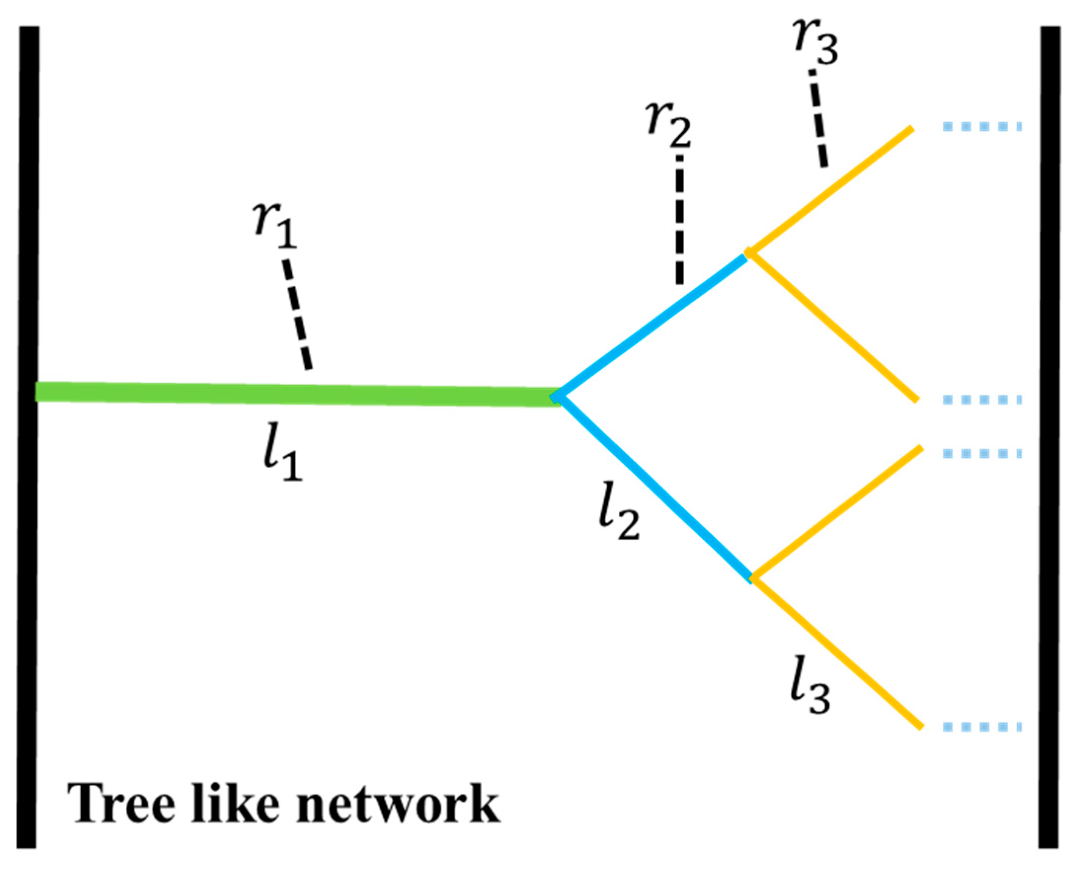
2. Assumptions and Models

In this section, a novel mathematical model of wetting phase imbibition into tree-like networks is proposed and the mechanisms of wettability alteration is considered. The tree-like network is shown in Figure 1. The wetting phase enters from the left side of the model and the capillary force and the imbibition speed change as wettability alteration occurs at different levels of the branched network. To compare with the Y-shaped branching model, we defined a control model called the capillary bundle model (as shown in Figure 2) and the following assumptions were made in regard to matching the models:

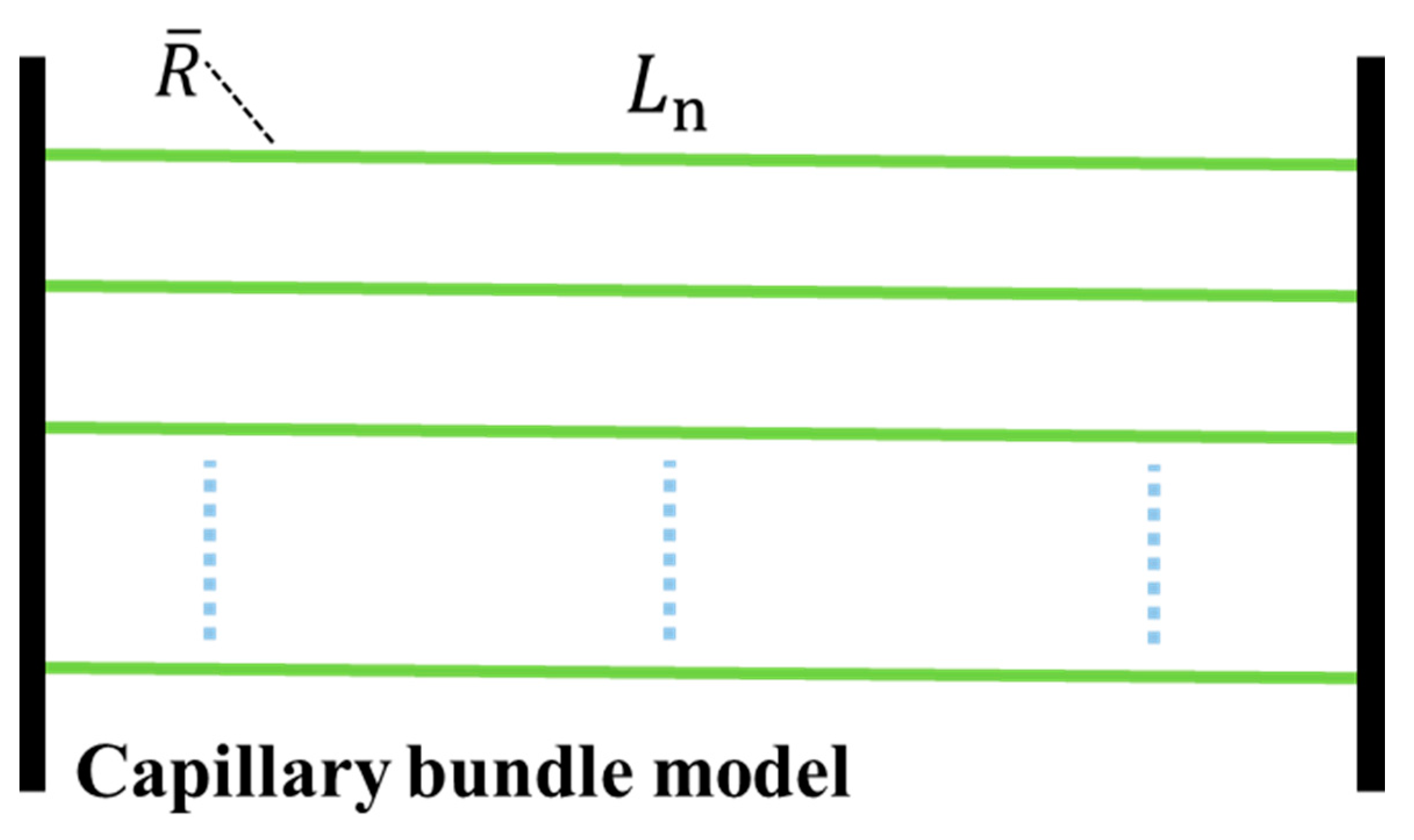
• The total length of the capillary tube is the same as that of the Y-shaped branching model;
• The specific surface area of the capillary bundle model is equal to that of the Y-shaped branching model, and the radius of the capillary bundle model is determined by this feature;
• The porosity of the capillary bundle model is equal to that of the Y-shaped branching model. According to the same porosity, the number of capillaries is determined;
• The permeability of the capillary bundle model is equal to that of the Y-shaped branching model. By keeping the specific surface area and porosity of the two models equal, the permeability of the two models is approximately equal.

The dynamics of capillary flow in a straight tube driven by the negative capillary pressure has been established and a correlation between the distance of liquid movement z and the time t has been proposed by Washburn [20].

$$z={(\frac{\gamma r\cos \theta }{2\eta }t)}^{0.5}$$

(1)

However, Washburn’s model is not based on describing the imbibition of complex porous media.

As shown in Figure 1, a network model with fractal characteristics is assumed and the wetting strength of each branch is different. It is called the Y-shaped branching model because the branching resembles a multi-stage Y-shape. The different branch colors represent the different wetting strengths of each level. Y-shaped branching networks with different wetting strengths are widely found in the development of tight sandstone reservoirs.

In Figure 1, the branches are composed of straight hollow tubes. Each branch is divided into m lower branches in the network system. By repeating this process, the network can be generated from the first-level branch to the nth-level branches, where n is the total number of branching levels.

The ratio of the radius between the (j + 1)th branch and jth branch is defined as Equation (2).

$$\alpha =r_{j+1}/r_j$$

(2)

and thus,

$$r_j={\alpha }^{j-1}{r}_1$$

(3)

where $r_j$ and $r_1$ are the radii of the tubes at the jth and the first branching levels, respectively. $\alpha$ is generally assumed to be smaller than 1 as in natural network systems.

Similarly, the ratio of the length of the tubes at the (j + 1)th branching level to that at the jth branching level is defined as Equation (4).

$$\beta =l_{j+1}/l_j$$

(4)

and therefore, it is easy to obtain Equation (5).

$$l_j={\beta }^{j-1}{l}_1$$

(5)

where $l_j$ and $l_1$ are the lengths of the tubes at the jth and first branching levels, respectively.

3. Derivation and Calculation

3.1. Model Features

In this work, we focused on investigating the capillary flow in the Y-shaped branching model whose tube length is greater than the radius. Y-shaped tree-like networks are widely found as natural and hydraulic fractures in the reservoir. In the model, the effect of the nodes between different branching levels on the flow is assumed negligible.

Based on Equation (4), the total length of the Y-shaped branching model is given by

$$L_{\mathrm{n}}={\displaystyle \sum _{j=1}^n{l}_j=\frac{1-{\beta }^n}{1-\beta }{l}_1}$$

(6)

The specific surface area of the capillary bundle model is calculated as Equation (7).

$$S_V=\frac{{\displaystyle {\sum }_{j=1}^{n}2\pi k_j{r}_j{l}_j}}{{\displaystyle {\sum }_{j=1}^n\pi k_j{r}_j^2{l}_j}}=\frac{2}{r_1}\frac{1-{\left(m\alpha \beta \right)}^n}{1-m\alpha \beta }\frac{1-m{\alpha }^2\beta }{1-{\left(m{\alpha }^2\beta \right)}^n}$$

(7)

where n is the total number of branching levels; m is the number of lower branches from an upper branch; $k_j$ is the number of branches at level j.

The specific surface area of the capillary bundle model is given by

$$S_V=\frac{k_{n}2\pi \overline{R}{L}_n}{k_n\pi {\overline{R}}^2{L}_n}=\frac{2}{\overline{R}}$$

(8)

where $\overline{R}$ is the branching radius of the capillary bundle model. According to Equations (7) and (8), it can be obtained that $\overline{R}$ is

$$\overline{R}=r_1\frac{1-m\alpha \beta }{1-{\left(m\alpha \beta \right)}^n}\frac{1-{\left(m{\alpha }^2\beta \right)}^n}{1-m{\alpha }^2\beta }$$

(9)

The total volume of the Y-shaped branching model is calculated as Equation (10).

$$V_{\mathrm{n}}={\displaystyle \sum _{j=1}^n\pi k_j{r}_j^2{l}_j=\pi r_1^2}{l}_1\frac{1-{\left(m{\alpha }^2\beta \right)}^n}{1-m{\alpha }^2\beta }$$

(10)

where $k_j$ is the number of tubes at the jth level, which is expressed as $k_j=m^{j-1}$.

The capillary bundle model has the same volume as the Y-shaped branching model, and the volume of the capillary bundle model is given by

$$V_n=\pi \overline{k}{\overline{R}}^2{L}_n$$

(11)

where $\overline{k}$ is the branch number of the model. Through Equations (9)–(11), it can be obtained that $\overline{k}$ is

$$\overline{k}=\frac{{\displaystyle {\sum }_{j=1}^n{k}_j{r}_j^2{l}_j}}{L_n{\overline{R}}^2}=\pi \frac{\left(1-m{\alpha }^2\beta \right)}{1-{\left(m{\alpha }^2\beta \right)}^n}\frac{1-\beta }{1-{\beta }^n}{\left(\frac{1-{\left(m\alpha \beta \right)}^n}{1-m\alpha \beta }\right)}^2$$

(12)

To make it easier to derive the formula, we defined that the wetting strength varies proportionally in the branching model. We defined the wettability coefficient S as the ratio of the $\cos \theta$ between the (j + 1)th branch and the jth branch,

$$s=\cos {\theta }_{j+1}/\cos {\theta }_j$$

(13)

and thus,

$$\cos {\theta }_j=s^{j-1}\cos {\theta }_1$$

(14)

3.2. Derivation of Flow Process

The capillary flow in each branch is driven by capillary pressure in the Y-shaped model. When the interface is in the kth branch, the capillary pressure is

$$\Delta p_{c,k}=-\frac{2\gamma \cos {\theta }_{\mathrm{k}}}{r_k}$$

(15)

The flow rate of the branch in the model is

$$Q=\pi r_{}^{2}u=-\frac{\pi r_{}^4}{8\eta }\frac{\partial p}{\partial x}$$

(16)

Based on Equations (1), (15), and (16) (summarized in Equation (17)), we performed a series of derivations to obtain Equation (18) (the detailed derivation process is shown in Appendix A).

$$\{\begin{array}{l}z={(\frac{\gamma r\cos \theta }{2\eta }t)}^{0.5}\\ \Delta p_{c,k}=-\frac{2\gamma \cos {\theta }_{\mathrm{k}}}{r_k}\\ Q=\pi r_{}^{2}u=-\frac{\pi r_{}^4}{8\eta }\frac{\partial p}{\partial x}\end{array}$$

(17)

The time $t_j$ required for the liquid to fill the tubes of the jth level with the length $l_j$ is obtained as Equation (18).

$$t_j=\frac{2\eta }{\gamma \cos {\theta }_j}\frac{l_j^2}{r_j}+\frac{4\eta }{\gamma \cos {\theta }_j}{\displaystyle \sum _{k=2}^j\left(m^{j+1-k}\frac{r_j^3{l}_{k-1}{l}_j}{r_{k-1}^4}\right)}$$

(18)

The total time $T_n$ required for the liquid to move distance $L_n$ is shown in Equation (19).

$$T_n={\displaystyle \sum _{j=1}^n{t}_j}=\frac{2\eta }{\gamma }{\displaystyle \sum _{j=1}^n\frac{1}{\cos {\theta }_{\mathrm{j}}}\frac{l_j^2}{r_j}}+\frac{4\eta }{\gamma }{\displaystyle \sum _{j=2}^n\frac{1}{\cos {\theta }_{\mathrm{j}}}{\displaystyle \sum _{k=2}^j\left(m^{j+1-k}\frac{r_j^3{l}_{k-1}{l}_j}{r_{k-1}^4}\right)}}$$

(19)

Then, when the liquid flows to the jth stage of the Y-shaped branching model and the total flow distance is l, the corresponding time $t_{l,j}$ is

$$t_{l,j}=\frac{2\eta }{\gamma \cos {\theta }_{\mathrm{j}}}\frac{{\left(l-L_{j-1}\right)}^2}{r_j}+\frac{4\eta }{\gamma \cos {\theta }_{\mathrm{j}}}{\displaystyle \sum _{k=2}^j\left[m^{j+1-k}\frac{r_j^3{l}_{k-1}\left(l-L_{j-1}\right)}{r_{k-1}^4}\right]}+T_{j-1}$$

(20)

By substituting Equations (3)–(5) into Equation (19), the relationship between $T_n$ and $\alpha$,$\beta$ is obtained as Equation (21).

$$T_n=\frac{2\eta }{\gamma \cos {\theta }_1}\frac{l_1^2}{r_1}\frac{1-{\left({\alpha }^{-1}{\beta }^2{\mathrm{s}}^{-1}\right)}^n}{1-{\alpha }^{-1}{\beta }^2{\mathrm{s}}^{-1}}+\frac{4\eta }{\gamma \cos {\theta }_1}\frac{l_1^2}{r_1}\frac{K}{1-{\alpha }^{-4}{m}^{-1}\beta }$$

(21)

where $K=\left[\frac{{\alpha }^{3}m\beta {\mathrm{s}}^{-1}-{\left({\alpha }^{3}m\beta {\mathrm{s}}^{-1}\right)}^n}{1-{\alpha }^{3}m\beta {\mathrm{s}}^{-1}}-\frac{{\alpha }^{-1}{\beta }^2{\mathrm{s}}^{-1}-{\left({\alpha }^{-1}{\beta }^2{\mathrm{s}}^{-1}\right)}^n}{1-{\alpha }^{-1}{\beta }^2{\mathrm{s}}^{-1}}\right]$.

Based on Equation (1), the total time for the liquid to fill the branches can be calculated in the capillary bundle model, as shown in Equation (22).

$$T_0=\frac{2\eta }{\gamma \cos {\theta }_1}\frac{L_n^2}{\overline{R}}=\frac{2\eta }{\gamma \cos {\theta }_1}\frac{l_1^2}{r_1}\frac{{\left(\frac{1-{\beta }^n}{1-\beta }\right)}^2}{\left[\frac{1-\mathrm{m}\alpha \beta }{1-{\left(m\alpha \beta \right)}^n}\frac{1-{\left(m{\alpha }^2\beta \right)}^n}{1-m{\alpha }^2\beta }\right]}$$

(22)

The dimensionless time of a capillary flow is defined as the ratio of Equations (21) and (22) in the Y-shaped branching model:

$$T_d=\frac{T_n}{T_0}=\frac{\left[\frac{1-\mathrm{m}\alpha \beta }{1-{\left(m\alpha \beta \right)}^n}\frac{1-{\left(m{\alpha }^2\beta \right)}^n}{1-m{\alpha }^2\beta }\right]\left\{\frac{1-{\left({\alpha }^{-1}{\beta }^2{\mathrm{s}}^{-1}\right)}^n}{1-{\alpha }^{-1}{\beta }^2{\mathrm{s}}^{-1}}+\frac{2}{1-{\alpha }^{-4}{m}^{-1}\beta }K\right\}}{{\left(\frac{1-{\beta }^n}{1-\beta }\right)}^2}$$

(23)

In the formula, $K=\left[\frac{{\alpha }^{3}m\beta {\mathrm{s}}^{-1}-{\left({\alpha }^{3}m\beta {\mathrm{s}}^{-1}\right)}^n}{1-{\alpha }^{3}m\beta {\mathrm{s}}^{-1}}-\frac{{\alpha }^{-1}{\beta }^2{\mathrm{s}}^{-1}-{\left({\alpha }^{-1}{\beta }^2{\mathrm{s}}^{-1}\right)}^n}{1-{\alpha }^{-1}{\beta }^2{\mathrm{s}}^{-1}}\right]$ indicates that the imbibition rate of the Y-shaped branching model is faster than that of the capillary bundle model, while $T_d$ is less than 1.

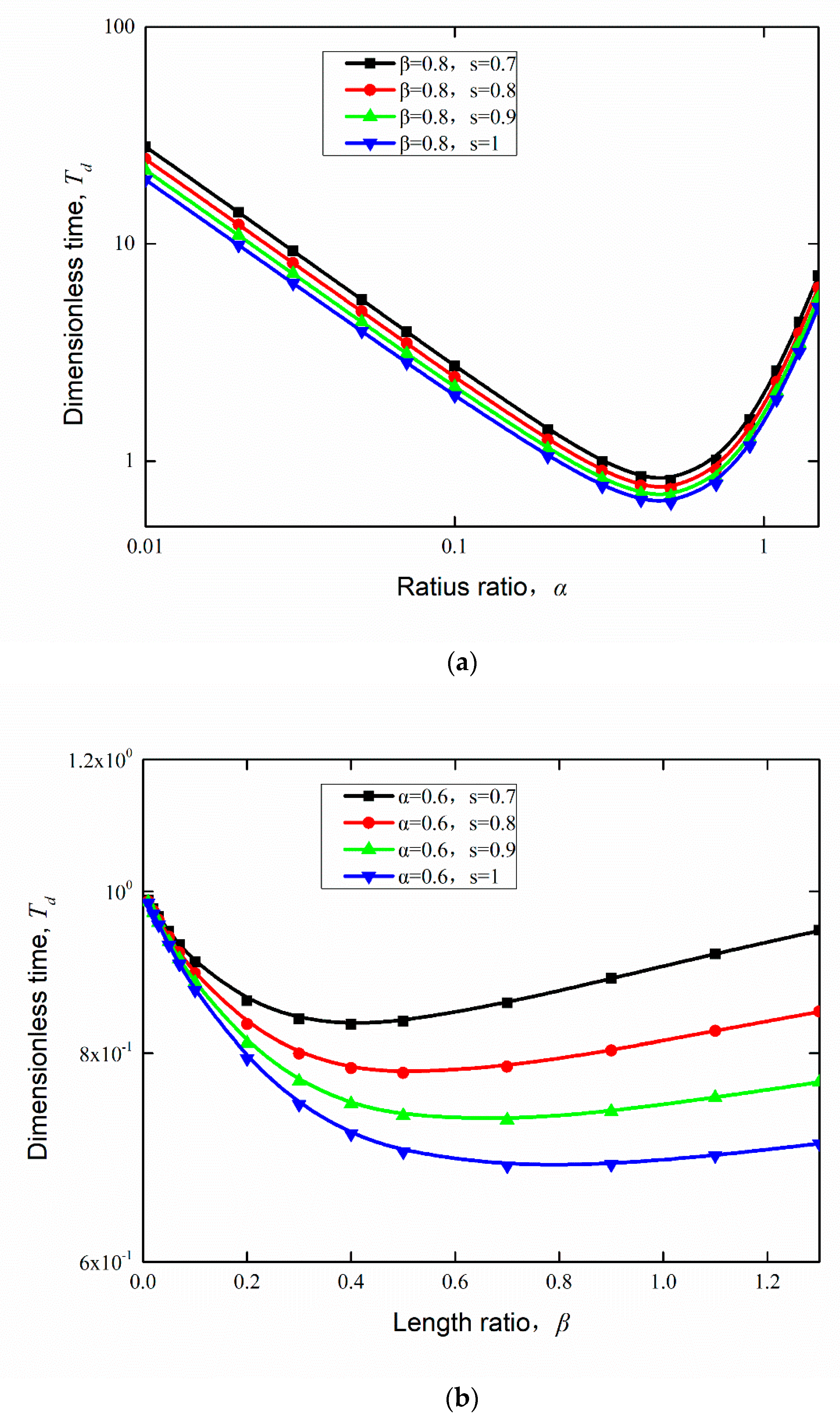
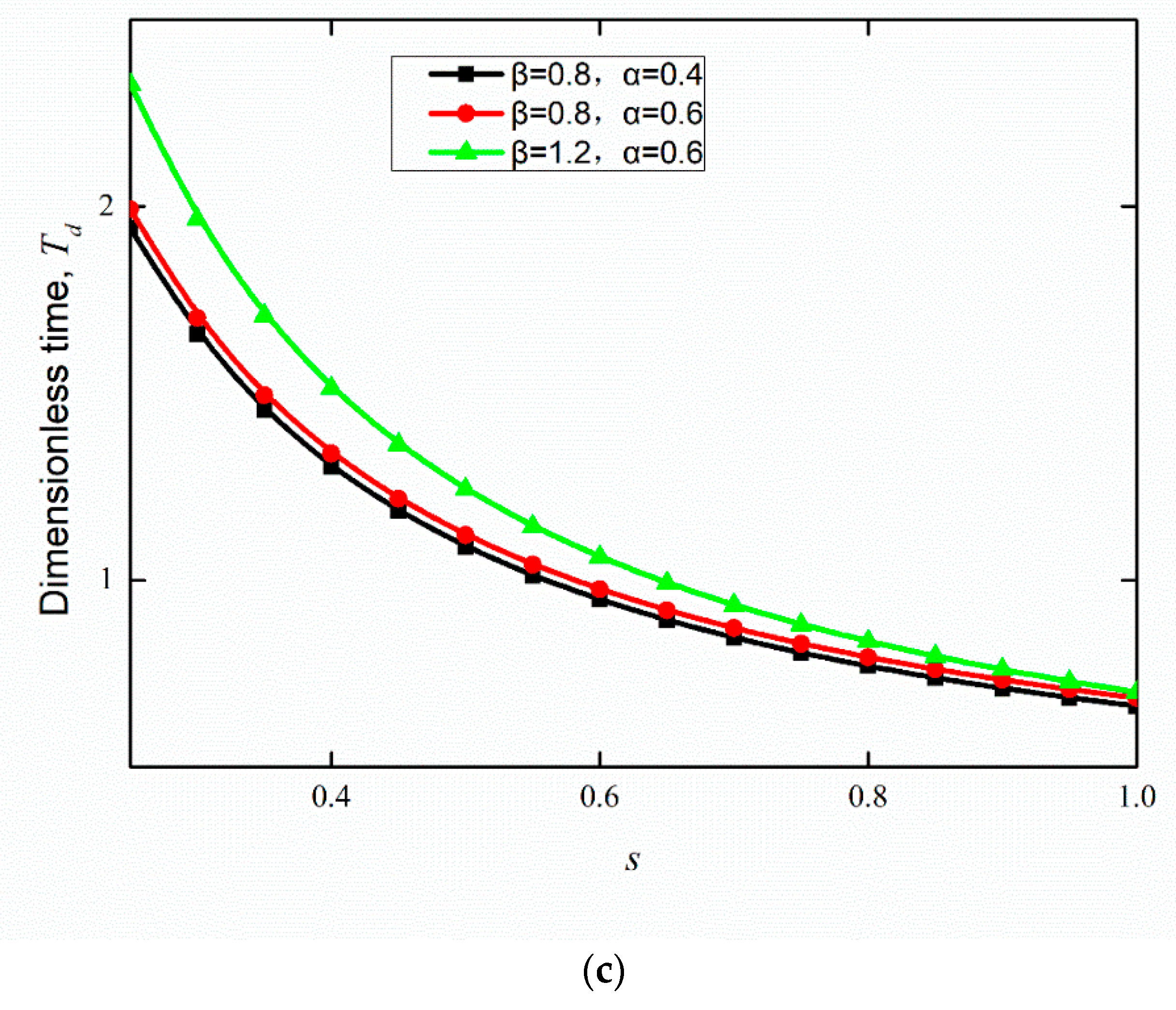
4. Results and Discussions

4.1. Effect of Proportional Variation in Wetting Strength on the Flow

In this section, we mainly studied the Y-shaped branching models with spatially varying wettability and the number of branches m = 2. From Figure 3 (n = 2), Figure 4 (n = 3) to Figure 5 (n = 4), the variation in the dimensionless time curves of the capillary flow (obtained from Equation (23)) with respect to the radius ratio $\alpha$, the length ratio $\beta$, and the wettability coefficient $s$ is clearly observed.

Figure 3a shows the curve of dimensionless time $T_d$ changing with the length ratio of $\alpha$ under different $s$ values in the two-level model. In Figure 3a, with the increase in $\alpha$, the dimensionless time curve first decreases sharply, reaches the lowest point when $\alpha$ approaches 0.5, and then increases sharply at all four different values of s (i.e., s = 0.7, 0.8, 0.9, and 1.0). Therefore, it can be seen from the curve that the optimal $\alpha$ is close to 0.4 for the minimum time required for the liquid to reach the end of the second branch in Figure 3a. It is also indicated that the decrease in s value leads to the increase in dimensionless time at the same radius ratio $\alpha$. However, the change in wettability coefficient s only causes the curve to shift up and down and has no influence on the trend of the curve with the radius ratio $\alpha$.

Figure 3b also shows that the constant decrease in the wettability coefficient s leads to the increase in dimensionless time when other parameters remain fixed. However, when $\beta$ approaches 0, the length of the secondary branch is close to 0, and the whole model becomes a uniform straight tube with the same wetting strength. Thus, for four different wettability coefficients s (i.e., s = 0.7, 0.8, 0.9, and 1.0), $T_d$ converges to the same value. When the length ratio $\beta$ grows larger, due to the increasing length of the secondary branch, the influence of different wetting strengths on capillary imbibition occurs gradually, and the difference between the curves gradually increases. Although the four curves with different s values vary in different ranges, the trend of the curves is almost the same.

In Figure 3c, it is found that the dimensionless time decreases gradually as the wettability coefficient s (s < 1) increases for an unchanged radius ratio and length ratio. The reason is that the improvement of wetting strength leads to the increase in capillary force and a faster imbibition rate. The change in the above curve is consistent with the change in dimensionless time when the s value increases in Figure 3a,b. It can be seen that as the s value increases, the amplitude of the dimensionless time change is smaller. The variation range of dimensionless time at s > 0.9 is much less than that at s < 0.4, so we considered that dimensionless time is approximately unchanged at s > 0.9. In addition, with the increase in wetting strength coefficient s, the law of dimensionless time variation does not change for different radius ratios $\alpha$ and length ratios $\beta$.

The $\alpha$, $\beta$, and s values at the minimum dimensionless time $T_d$ can be obtained from Figure 3. In addition, the minimum dimensionless time $T_d$ = 0.6362 can be calculated precisely under the conditions of s = 1, $\alpha$ = 0.4603, and $\beta$ = 0.6203. Under the same conditions of length, volume, and specific surface, the spontaneous imbibition time $T_d$ of the two-stage branching model is 36.38% lower than that of the capillary bundle model.

Similar to the two-stage branching model with different wetting strengths, the effects of the variations in $\alpha$,$\beta$, and s on dimensionless time $T_d$ are shown, respectively, in Figure 4a–c when the total number of branching levels n is 3. Although the capillary flow variation corresponding to $\alpha$ and $\beta$ in the three-stage branch network has the same trend as that in the two-stage network, the optimal solutions for $\alpha$, $\beta$, and s are different from those for the two-stage network. The minimum dimensionless time $T_d=0.5154$ is calculated precisely under the conditions of s = 1, $\alpha$ = 0.5143, and $\beta$ = 0.6557. Under the same conditions of length, volume, and specific surface, the spontaneous imbibition time $T_d$ of the three-stage branching model is 48.46% lower than that of the capillary bundle model.

When the total number of branching levels n is 3 to 4, the minimum dimensionless time $T_d$ and the corresponding $\alpha$, $\beta$, and s are all changed, where $T_d=0.4518$, s = 1, $\alpha$ = 0.5567, and $\beta$ = 0.6896. Under the same conditions of length, volume, and specific surface, the spontaneous imbibition time $T_d$ of the four-stage branching model is 54.82% lower than that of the capillary bundle model. According to the above curve, a conclusion can be drawn: under the condition that s = 1 (with same wetting strength), the shortest time $T_d$ can be obtained, and the fluid imbibition speed in the multi-stage branching model will be faster.

In order to make a comparison between a capillary bundle model, which is restricted by the same length, porosity, and permeability as the tree-like network model (s = 1), the dimensionless imbibition time was calculated for different dimensionless distances l_d. The dimensionless distance l_d is the total length of the Y-shaped branching model divided by the length of the first branch, which is normalized to avoid the value of the model length and to facilitate the comparison under different conditions. The relationship between dimensionless time T_d and dimensionless length l_d is shown in Figure 6. The result confirms that the imbibition process in the capillary bundle model obeys the rule described by the Washburn equation. However, the imbibition in the tree-like network model did not obey the Washburn equation. With the same l_d, a shorter imbibition time was observed in the tree-like network model. The minimum dimensionless time T_d = 0.5154 was calculated precisely under the conditions of s = 1, α = 0.5143, and β = 0.6557. Hence, the imbibition process can be accelerated in the tree-like network models.

4.2. Effect of Random Variation in Wetting Strength on Flow

In the previous section, the variation trend of spontaneous imbibition time with radius ratio $\alpha$, length ratio $\beta$, and wettability coefficient s in the multi-stage branching model was discussed. However, wettability hardly varies proportionately, and more random variation is observed in the pore space of the real tight sandstone reservoir. Therefore, in this section, a three-stage Y-shaped branching model is used to study the fluid imbibition qualitatively when the wetting strength changes randomly in the pore space of tight sandstone.

We assumed six random realizations of wettability variations and divided them into two groups for analysis (as shown in

Table 1. Cases of random variation in wetting strength.

	Case No.	cosθ1	cosθ2	cosθ3
First Group	#1	0.8	0.2	0.2
	#2	0.2	0.8	0.2
	#3	0.2	0.2	0.8
Second Group	#4	0.2	0.8	0.8
	#5	0.8	0.2	0.8
	#6	0.8	0.8	0.2

). The two groups of experiments investigated the change in spontaneous imbibition time with distance when the wettability of a certain branch suddenly becomes stronger or weaker.

In the first group, it is assumed that the wettability of the first-, second-, or third-stage branch is strong when other branches’ wettability is generally weak in the model. In assumption 1, the wettability in the first-, second-, and third-stage branches is strong, weak, and weak, respectively. This means that the wetting strength of the first stage in the model is relatively large, which differs from those of the other branches. In assumption 2, the wettability in the first, second, and third stages is weak, strong, and weak, respectively. This shows that the wetting strength of the second stage’s branch is larger than those of the other branches. In assumption 3, similarly, the wetting strength of the third stage is larger than those of the other stages and the order of the wettability is weak, weak, and strong. By comparing the three assumptions, the effect of the wettability of a certain branch becomes stronger on the overall imbibition time and the sensitivity of each branch to the wettability change can be obtained.

According to Equation (18), the relationship between flow time and flow distance of the first group is shown in Figure 7 when the length ratio and radius ratio are the optimal solutions in the three-level branching model. It is easily observed that, compared with the branch tubes with weak wetting strength, the branch tubes with strong wetting strength have a strong capillary force and a faster flow of fluid, which causes a significantly shorter time of fluid imbibition.

The shortest imbibition time is obtained in realization 2. The fluid flows through the first-stage branch for a longer time in realization 2. However, the flow time of realization 2 is still shortest as the fluid flows faster and more time is shortened in the second-stage branch. In addition, the longest flow time occurs in realization 1. We compared the three curves and found that the flow time is most sensitive to the wettability of the second branch in the three-level branch model.

In the second group, the assumption is opposite to the first group. It was assumed that the wettability of the model is generally strong but the wettability of the first, second, or third stage branches change suddenly and become weak. Realization 4 is that the wettability of the first-stage branches becomes weak. Similarly, realization 5 is that the wettability of the second-stage branches becomes weak. In addition, the order of the wettability is strong, strong, and weak in realization 6.

According to Equation (18), the relationship between flow time and flow distance of the second group is shown in Figure 8 when the length ratio and radius ratio are the optimal solutions. It can be seen that the flow time of the fluid in the branch tube with weak wetting strength is significantly longer and the flow velocity of the fluid is lower.

Comparing the ordinates of the three curves, it is obvious that realization 5 has the longest time, and the shortest time occurs in realization 4. This phenomenon means that the flow time is most sensitive to the wettability of the second branch, which is consistent with the findings of the first group.

The first group assumes that the wetting strength is randomly weakened, and the second group assumes that the wetting strength is randomly strengthened. By comparing the two groups and considering the above curve analysis, the following conclusions can be drawn: (1) The strong wettability branch can accelerate the capillary fluid imbibition, while the weak wettability branch can slow down the capillary fluid imbibition. (2) In the three-stage branching model, the dimensionless time is most sensitive to the wettability of the second branch for liquid spontaneous imbibition when the length ratio and radius ratio are the optimal solutions. (3) In the approximate three-level branching model, we should first consider the second-level branch, which will cause great changes in the results if wetting strength is to be changed.

5. Conclusions

In this paper, a new physical model considering wettability and permeability for the Y-shaped branch model was established. The capillary bundle model was designed as the control model, and the mathematical formulas of dimensionless time and other flow characteristics of the branch model in the branch model were derived. In the case that the ratio of radius $\alpha$ and ratio of length $\beta$ are defined, the variation trend of dimensionless time T_d and the time of fluid flow to the end of the model with different wettabilities were studied, and the sensitivity of dimensionless time to wettability changes was investigated. A three-stage branching model was selected to investigate the dynamics of capillary flow with random wettability changes. This paper shows the law of spontaneous imbibition of Newtonian fluids in Y-shape branching models with different wettabilities, which is of significance for the study of fluid flow in the pore space of tight sandstone reservoirs.

References

1. Berkowitz, B.; Ewing, R.P. Percolation Theory and Network Modeling Applications in Soil Physics. Surv. Geophys. 1998, 19, 23–72. [Google Scholar] [CrossRef]
2. Zhang, L.; Xu, C.; Guo, Y.; Zhu, G.; Cai, S.; Wang, X.; Jing, W.; Sun, H.; Yang, Y.; Yao, J. The Effect of Surface Roughness on Immiscible Displacement Using Pore Scale Simulation. Transp. Porous Media 2021, 1–13. [Google Scholar] [CrossRef]
3. Yang, Y.F.; Liu, J.; Yao, J.; Kou, J.L.; Li, Z.; Wu, T.H.; Zhang, K.; Zhang, L.; Sun, H. Adsorption behaviors of shale oil in kerogen slit by molecular simulation. Chem. Eng. J. 2020, 387, 124054. [Google Scholar] [CrossRef]
4. Yang, Y.F.; Yang, H.Y.; Tao, L.; Yao, J. Microscopic Determination of Remaining Oil Distribution in Sandstones With Different Permeability Scales Using Computed Tomography Scanning. J. Energy Resour. Technol.-Trans. ASME 2019, 141, 092903. [Google Scholar] [CrossRef]
5. Yang, Y.F.; Yao, J.; Wang, C.C.; Gao, Y.; Zhang, Q.; An, S.Y.; Song, W.H. New pore space characterization method of shale matrix formation by considering organic and inorganic pores. J. Nat. Gas Sci. Eng. 2015, 27, 496–503. [Google Scholar] [CrossRef]
6. Balberg, I.; Berkowitz, B.; Drachsler, G.E. Application of a percolation model to flow in fractured hard rocks. J. Geophys. Res. Solid Earth 1991, 96, 10015–10021. [Google Scholar] [CrossRef]
7. Liu, J.; Regenauer-Lieb, K. Application of percolation theory to microtomography of rocks. Earth-Sci. Rev. 2021, 214, 103519. [Google Scholar] [CrossRef]
8. Cai, J.; Jin, T.; Kou, J.; Zou, S.; Xiao, J.; Meng, Q. Lucas-Washburn Equation-Based Modeling of Capillary-Driven Flow in Porous Systems. Langmuir 2021, 37, 1623–1636. [Google Scholar] [CrossRef] [PubMed]
9. Meng, Q.; Cai, J. Recent advances in spontaneous imbibition with different boundary conditions. Capillarity 2018, 1, 19–26. [Google Scholar] [CrossRef] [Green Version]
10. Zhang, L.; Jing, W.L.; Yang, Y.F.; Yang, H.N.; Guo, Y.H.; Sun, H.; Zhao, J.L.; Yao, J. The Investigation of Permeability Calculation Using Digital Core Simulation Technology. Energies 2019, 12, 3273. [Google Scholar] [CrossRef] [Green Version]
11. Parteli, E.J.R.; da Silva, L.R.; Andrade, J.S., Jr. Self-organized percolation in multi-layered structures. J. Stat. Mech. Theory Exp. 2010, 2010, P03026. [Google Scholar] [CrossRef] [Green Version]
12. Kuuskraa, V.; Stevens, S.H.; Moodhe, K.D. Technically Recoverable Shale Oil and Shale Gas Resources: An Assessment of 137 Shale Formations in 41 Countries outside the United States; Adiministation, U.S. Energy Information: Washington, DC, USA, 2013.
13. Li, N.; Ran, Q.; Li, J.; Yuan, J.; Wang, C.; Wu, Y.-S. A Multiple-Continuum Model for Simulation of Gas Production from Shale Gas Reservoirs. In Proceedings of the All Days, Abu Dhabi, United Arab Emirates, 16 September 2013; p. 13. [Google Scholar]
14. Yang, Y.F.; Wang, K.; Zhang, L.; Sun, H.; Zhang, K.; Ma, J.S. Pore-scale simulation of shale oil flow based on pore network model. Fuel 2019, 251, 683–692. [Google Scholar] [CrossRef]
15. Cao, Y.; Tang, M.; Zhang, Q.; Tang, J.; Lu, S. Dynamic capillary pressure analysis of tight sandstone based on digital rock model. Capillarity 2020, 3, 28–35. [Google Scholar] [CrossRef]
16. Gao, L.; Yang, Z.; Shi, Y. Experimental study on spontaneous imbibition characteristics of tight rocks. Adv. Geo-Energy Res. 2018, 2, 292–304. [Google Scholar] [CrossRef]
17. Cai, J.; Yu, B. Advances in studies of spontaneous imbibition in porous media. Adv. Mech. 2012, 42, 735–754. [Google Scholar] [CrossRef]
18. Meng, Q.; Liu, H.; Wang, J. A critical review on fundamental mechanisms of spontaneous imbibition and the impact of boundary condition, fluid viscosity and wettability. Adv. Geo-Energy Res. 2017, 1, 1–17. [Google Scholar] [CrossRef]
19. Lucas, R. Rate of capillary ascension of liquids. Kolloid Z. 1918, 23, 15–22. [Google Scholar] [CrossRef]
20. Washburn, E.W. The Dynamics of Capillary Flow. Phys. Rev. 1921, 17, 273–283. [Google Scholar] [CrossRef]
21. Terzaghi, K. Theoretical Soil Mechanics; Wiley: New York, NY, USA, 1943. [Google Scholar]
22. Handy, L.L. Determination of Effective Capillary Pressures for Porous Media from Imbibition Data. Trans. AIME 1960, 219, 75–80. [Google Scholar] [CrossRef]
23. Cuiec, L.E.; Bourbiaux, B.; Kalaydjian, F. Oil recovery by imbibition in low-permeability chalk. SPE Form. Eval. 1994, 9, 200–208. [Google Scholar] [CrossRef]
24. Kazemi, H.; Gilman, J.R.; Eisharkawy, A.M. Analytical and numerical solution of oil recovery from fractured reservoirs with empirical transfer functions. SPE Reserv. Eng. 1992, 7, 219–227. [Google Scholar] [CrossRef]
25. Li, K.W.; Horne, R.N. An analytical scaling method for spontaneous imbibition in gas/water/rock systems. SPE J. 2004, 9, 322–329. [Google Scholar] [CrossRef]
26. Li, K.W.; Horne, R.N. Generalized scaling approach for spontaneous imbibition: An analytical model. SPE Reserv. Eval. Eng. 2006, 9, 251–258. [Google Scholar] [CrossRef]
27. Mattax, C.C.; Kyte, J.R. Imbibition Oil Recovery from Fractured, Water-Drive Reservoir. Soc. Pet. Eng. J. 1962, 2, 177–184. [Google Scholar] [CrossRef]
28. Shouxiang, M.; Morrow, N.R.; Zhang, X. Generalized scaling of spontaneous imbibition data for strongly water-wet systems. J. Pet. Sci. Eng. 1997, 18, 165–178. [Google Scholar] [CrossRef]
29. Benavente, D.; Lock, P.; Del Cura, M.A.G.; Ordonez, S. Predicting the capillary imbibition of porous rocks from microstructure. Transp. Porous Media 2002, 49, 59–76. [Google Scholar] [CrossRef]
30. Leventis, A.; Verganelakis, D.A.; Halse, M.R.; Webber, J.B.; Strange, J.H. Capillary Imbibition and Pore Characterisation in Cement Pastes. Transp. Porous Media 2000, 39, 143–157. [Google Scholar] [CrossRef]
31. Li, Y.; Yu, D.; Niu, B. Prediction of spontaneous imbibition in fractal porous media based on modified porosity correlation. Capillarity 2021, 4, 13–22. [Google Scholar] [CrossRef]
32. Mandelbrot, B.B. The Fractal Geometry of Nature; Times Books: New York, NY, USA, 1982. [Google Scholar]
33. Wheatcraft, S.W.; Tyler, S.W. An explanation of scale-dependent dispersivity in heterogeneous aquifers using concepts of fractal geometry. Water Resour. Res. 1988, 24, 566–578. [Google Scholar] [CrossRef]
34. Cai, J.C.; Yu, B.M.; Zou, M.Q.; Luo, L. Fractal Characterization of Spontaneous Co-current Imbibition in Porous Media. Energy Fuels 2010, 24, 1860–1867. [Google Scholar] [CrossRef]
35. Wang, W.D.; Su, Y.L.; Zhang, X.; Sheng, G.L.; Ren, L. Analysis of the Complex Fracture Flow in Multiple Fractured Horizontal Wells with the Fractal Tree-Like Network Models. Fractals-Complex Geom. Patterns Scaling Nat. Soc. 2015, 23, 1550014. [Google Scholar] [CrossRef]
36. Li, C.; Shen, Y.; Ge, H.; Su, S.; Yang, Z. Analysis of Spontaneous Imbibition in Fractal Tree-Like Network System. Fractals 2016, 24, 1650035. [Google Scholar] [CrossRef] [Green Version]
37. Shou, D.; Ye, L.; Fan, J. Treelike networks accelerating capillary flow. Phys. Rev. E Stat. Nonlinear Soft Matter Phys. 2014, 89, 053007. [Google Scholar] [CrossRef] [PubMed]
38. Lin, D.; Wang, J.; Yuan, B.; Shen, Y. Review on gas flow and recovery in unconventional porous rocks. Adv. Geo-Energy Res. 2017, 1, 39–53. [Google Scholar] [CrossRef]
39. Buckley, J.S.; Liu, Y. Some mechanisms of crude oil/brine/solid interactions. J. Pet. Sci. Eng. 1998, 20, 155–160. [Google Scholar] [CrossRef]
40. Zhu, G.P.; Kou, J.S.; Yao, B.W.; Wu, Y.S.; Yao, J.; Sun, S.Y. Thermodynamically consistent modelling of two-phase flows with moving contact line and soluble surfactants. J. Fluid Mech. 2019, 879, 327–359. [Google Scholar] [CrossRef] [Green Version]
41. Zhu, G.P.; Kou, J.S.; Yao, J.; Li, A.F.; Sun, S.Y. A phase-field moving contact line model with soluble surfactants. J. Comput. Phys. 2020, 405, 109170. [Google Scholar] [CrossRef]
42. Yang, Y.; Cai, S.; Yao, J.; Zhong, J.; Zhang, K.; Song, W.; Zhang, L.; Sun, H.; Lisitsa, V. Pore-scale simulation of remaining oil distribution in 3D porous media affected by wettability and capillarity based on volume of fluid method. Int. J. Multiph. Flow 2021, 143, 103746. [Google Scholar] [CrossRef]
Figure 1. Y-shaped branching model.
Water 13 02370 g001
Figure 2. Capillary bundle model.
Water 13 02370 g002
Figure 3. Dimensionless time curves of capillary flow at n = 2. (a) The effect of radius ratio α at different s values, (b) the effect of length ratio β at different s values, and (c) the effect of radius s values at different radius ratios α and length ratios β.
Water 13 02370 g003aWater 13 02370 g003b
Figure 4. Dimensionless time curves of capillary flow at n = 3. (a) The curve of change with radius ratio α at different s values, (b) curve of change with length ratio β at different s values, (c) curve of change with radius s values at different radius ratios α and length ratios β .
Water 13 02370 g004aWater 13 02370 g004b
Figure 5. Dimensionless time curves of capillary flow at n = 4. (a) The curve of change with radius ratio α at different s values, (b) curve of change with length ratio β at different s values, (c) curve of change with radius s values at different radius ratios α and length ratios β .
Water 13 02370 g005aWater 13 02370 g005b
Figure 6. Comparison of Td from capillary bundle model and tree-like network model with changing ld.
Water 13 02370 g006
Figure 7. Dimensionless time varies with the distance of liquid flow in the first group of assumptions.
Water 13 02370 g007
Figure 8. Dimensionless time varies with the distance of fluid flow in the second group of realizations.
Water 13 02370 g008