Abstract
Although Austria is a water-rich country, impacts of climate change on water supply are already noticeable. Some regions were affected by water scarcity in recent years. Due to climate change, an increase in peak water demand is expected in the future. Therefore, water demand prediction models that include climate indices are of interest. In this paper, we present a general multiple linear regression (GMLR) model that can be applied to selected study sites. We compared the performance of the GMLR model with different modeling approaches, i.e., stepwise multiple linear regression, support vector regression, random forest regression and a neural network approach. All models were trained with water demand and weather data reaching back several years and tested with the last available observation year. The applied modeling approaches achieved a similar performance. As a second step, the GMLR model was used to estimate the peak water demands for the time period 2025–2050. For the future water demand estimate, 16 different climate projections were used. These climate projections represent the worst-case climate change scenario (RCP 8.5). The expected increase in peak water demand could be confirmed with the modeling approach. An increase in peak water demand by 3.5% compared to the reference period was estimated.
Keywords:
long-term daily water demand forecasting; peak water demand; climate change; MLR; SVR; RF; ANN 1. Introduction
Water demand is influenced by various trends, like climate change, economic change and demographic change [1,2]. These trends change slowly over several years, but still, have a major impact on future daily water demand. Countries all over the world will have to deal with the effects of these trends in the future. Although Austria is a water-rich country, some regions are affected by water shortages. These regions may face water scarcity in the future due to the trends mentioned before, if there is a strong population growth in some regions the water demand will increase, and this can lead to a supply shortage [3]. With regard to these changes, water utilities need to be able to estimate the future water demand. Therefore, long-term forecast models are necessary.
Most research on water demand forecasting can be divided into short-term or long-term forecasts. Short-term forecasts are mostly based on hourly or daily water demands and serve for operational optimization tasks. Almost all long-term forecasts deal with monthly or annual water demands [4].
There are several studies analyzing different modeling approaches for short-term water demand forecasting. Vijai and Bagavathi Sivakumar [5] compared modeling approaches for short-term prediction using hourly and daily interval data. The following approaches were used for this comparison: artificial neural network (ANN), deep neural network, extreme learning machine, least square support vector machine, Gaussian process regression and random forest (RF).
Support vector regression (SVR) and artificial neural networks are common modeling approaches for water demand prediction. Both approaches can be used for short-term and long-term predictions. In the study from Msiza et al. [6] both approaches were compared, and it was observed that the ANNs outperformed the SVMs. Zubaidi et al. [7] used an ANN to predict long-term, monthly water demands. The study has shown that the model achieved good results by comparing the observed and the predicted water demand. The authors pointed out that more research is required to learn more about the impacts and the relationships between climate change and long-term water demand for different regions.
A lot of research that deals with the effects of climate change on water demand can be found in the literature. A study for the city of Toronto [8] showed that the average summer water demand will increase by 2% and the peak water demand will increase by 1.8% if the daily maximum temperature rises by 1 °C in summer. In this study, a stepwise regression approach was used to derive a daily demand model. A long-term demand model was derived from the daily demand model. Donevska and Panov [9] used multiregression models to show the impact of climate change on water demand. Therefore, water supply data was considered in relation to the climate parameters (temperature and precipitation). Vonk et al. [10] predicted daily water demand with a SVR model, considering meteorological parameters and changes in vacation absence/presence (tourism) and coupled that to an extreme value model. The effects of different climate change and vacation scenarios for 2050 were predicted. They found that the average water demand increases by 0.8%, while the peak water demand increases by 6.5% by 2050.
A study [11] for Austria that describes the impact of climate on peak water demand indicates that effects depicted in [8,9,10] will likely occur here as well. In the Austrian study, the relationship between temperature, dry episodes and water demand was demonstrated. The authors found that daily water demand increases when the temperature rises. It was also shown that peak water demand occurs on days with increased temperatures.
Given these findings, utilities need appropriate models for long-term predictions and those models need to be able to incorporate climate change and sociodemographic development. The purpose of this work is to show the long-term changes in peak water demand using a general regression model. In many cases, only short water demand records are available, which makes the development of a general regression model difficult. Nevertheless, we aimed to derive a suitable and general regression model from zonal inflow data that were available in Austria. This model should be able to forecast future peak water demand (amount and frequency) with respect to climate projections. In a first step, the correlation between water demand and weather records is analyzed. For this short period a general regression model is developed using weather records, since climate projections are not suitable for this short-term analysis. In a next step the general regression model is applied to climate projections for a long-term estimate. A requirement is that the general regression model can be applied to different study sites in Austria. This is particularly important, as this model will be integrated into a game-based, strategic, long-term planning tool for water utilities. This serious game is being developed for a research project [12]. Among other things, this planning tool evaluates the long-term resilience of water supply systems for several climate change scenarios. In addition, the user can apply different urban and demographic development strategies. Therefore, a model that allows one to predict the peak water demand and the number of peak water demand days for different climate change and demographic scenarios is needed.
Given these goals and constraints, this work is structured as follows. In the materials and methods section, we give an overview of the study sites and the climate projections. Next, we briefly describe the workflow. In the results section, we present the performance evaluation of the general regression model and compare the results from the peak water demand forecast with the reference period, before drawing our conclusions in the final section.
2. Materials
2.1. Study Sites
For this work, two areas in Austria were selected, Vienna and Graz. Vienna’s water distribution system is divided into measurement zones. For the use in our research, inflow data for two individual zones were available. For both zones, the inflow into the zone is measured. While the first zone (Zone 1) is a residential district with detached houses, the second (Zone 2) is composed of both residential and industrial use. The mean inflow in Zone 1 is 4871 m3/d and 5109 m3/d in Zone 2.
For Graz inflow data for two zones were provided by the utility. Both zones are residential districts. The mean inflow for Zone 3 is 2015 m3/d and 2259 m3/d for Zone 4. The measurement devices are positioned at pumping stations. In both zones, counter tanks are located in the system. Therefore, not only the consumption in this zone is measured, but also the counter tank filling is shown in the inflow measurement. The tank fillings do not follow any recognizable pattern and information about pumping schedules was not available. The demographics composition in the selected zones is representative of many other zones in Austria.
2.2. Water Demand and Weather Records
2.2.1. Water Demand Records
Water utilities in Austria keep records of daily water demand, represented by daily system or zone inflow. These records reflect an approximation of the actual water demand for the supplied area, when assuming that water losses are small and constant over the measured period due to active leakage control. There are no fluctuations due to tourism in the selected zones.
In a preliminary analysis, we analyzed the monthly water demand of the four different study sites for an observation period of several years. The purpose was to derive if and in which months an increase in demand can be observed. From the available inflow data, we could derive that during the winter months (October–March) the water demand is generally lower than during the rest of the year. For example, Figure 1 shows a heat map of the maximum daily demand per month from 2013 to 2019 in Zone 4.
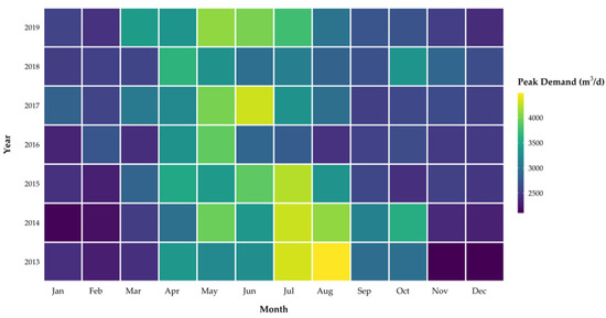
Figure 1.
Maximum daily water demand per month for Zone 4. The lighter the color the higher the water demand.
For further analysis only a short period (three years from 2017 to 2019) of water demand records were considered because this time series was available for all zones without larger gaps. In addition, the water distribution network structure and operation system did no notable change during this period. Additionally, in these three years the amount and categories of customers did not change.
In the study period, the mean daily water demand in Zone 4 during the winter months was 2292 m3/d and during the summer months it was 2637 m3/d. As the peak water demand days are especially interesting for our research, we made the following assumptions: All days, where the daily demand falls within the upper 10% range of the daily demand of the observation period, were considered and labeled as peak water demand days. In the period from 2017 to 2019, 58 peak water demand days were measured for Zone 4. These occurred as follows, 11 in April, 18 in May, 21 in June and 8 in July. For this zone none occurred in August and September. Comparing the number and amount of peak water demand days with those of Zone 1, the distribution looked somewhat different. The mean daily water demand during the winter months was 4714 m3/d, while the mean daily water demand was 5006 m3/d during the summer months. In Zone 1 a total of 67 peak water demand days were recorded. Out of these 67 days, 3 occurred in April, 11 in May, 41 in June, 7 in July and 5 in August. No peak water demand day occurred in September, but the demand was still higher than in the following months.
As our goal was to determine the number of days with the highest demand and how they are related to climate indices like hot days and consecutive dry days, we limited the observation period to the months April to September.
2.2.2. Weather Records
Daily weather records for the observation period 2017–2019 were obtained from the Central Institute for Meteorology and Geodynamics (ZAMG) [13]. These weather records include mean temperature, maximum temperature, minimum temperature, amount of precipitation and the kind of precipitation. For each water supply system, the data from the closest meteorological station were used. For the study site in Graz, we used precipitation records from a nearby weather station, which were collected by Maier et al. [14]. Weather records were used to show the relationship between weather phenomena and water demand.
2.3. Climate Change Scenarios
For the Intergovernmental Panel on Climate Change’s (IPCC) Fifth Assessment Report, representative concentration pathways (RCPs) were developed. The term “representative” describes that each RCP represents only one pathway of a large set of scenarios. Each scenario can lead to the specific characteristics of the radiation forcing. The word “pathway” describes that the long-term concentration levels and trajectory taken over time are important to achieve the result [15].
According to van Vuuren et al. [16], four RCPs were created in cooperation with emission inventory experts, terrestrial ecosystem modelers, integrated assessment modelers and climate modelers. The selected RCPs were named after the radiative forcing target level for the end of the 21st century. These pathways were expected to lead to a radiative forcing level of 2.6, 4.5, 6.0 and 8.5 W/m2 by 2100. The RCPs contained one mitigation scenario (RCP2.6), two medium stabilization scenarios (RCP4.5/RCP6.0) and one very high baseline emission scenario (RCP8.5).
The ÖKS 15 study [17] describes the impact of climate change on Austria. In this study, climate projections for Austria were created, which represent the RCPs. Climate projections are derived from various combinations of global (GCM) and regional climate models (RCM). The RCMs have been bias corrected by means of scaled distribution mapping. Each climate projection represents a plausible possible state of the climate The climate varies in a natural way, these variations are called climate variability. A 25- or 30-year period is needed to better compensate the short-term climate variability. If the climate projections were used for a shorter period, there are too many uncertainties due to the annual climate variability.
To describe the climate changes, 27 climate indices are defined in the ÖKS 15 study [17]. These indices are based on intuitive and statistically robust climate parameters that are either temperature, precipitation or radiation-based. Therefore, the 27 indices are divided into three groups, temperature-based, radiation-based and precipitation-based. The study describes that for the time period 2021–2050 an average increase of 11 summer days (days with a maximum temperature of more than 25.0 °C) and 4.3 hot days (days with a maximum temperature of more than 30.0 °C) can be expected in Austria for the RCP8.5. Furthermore, a rise in the mean air temperature of 1.4 °C on average can be expected for Austria. The climate projections are available on the CCCA Data Server platform [18]. The climate projections offer the unique possibility to look at global climate changes on a local level. Therefore, global changes can be represented without considering changes in the local demographic development.
Climate Classification
According to Rubel et al. [19], there are three different climates, Dfb, Cfb and ET, in Austria. The climate classification Dfb describes a humid and warm continental climate. Cfb classifies a warm temperate climate, fully humid and warm summers. The abbreviation ET stands for a tundra climate. The climate classification for Vienna and Graz is Cfb. Rubel at al. [19] showed how the climate classification can shift due to the different climate change scenarios in the alpine region and in Austria. For the worst-case climate change scenario, the climate classification Cfb could change to Cfa until the end of the 21st century. Cfa stands for warm temperate climate, fully humid and hot summers. For example, the current climate classification in Bologna is Cfa.
3. Methods
In this section, an insight into data preparation is given and then a brief overview of the three-step workflow of the modeling approach is provided. Figure 2 presents a flowchart where the three steps are described.
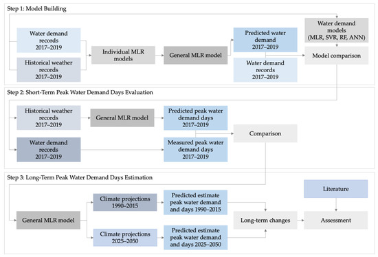
Figure 2.
Model building workflow. The model building process is split up into three steps. First model building, second short-term peak water demand days evaluation and last long-term peak water demand days estimation.
In the first step, a general multiple linear regression (GMLR) model was derived from individual MLR models using the short-term water demand and weather datasets. The weather records were used, because climate projections are not suitable for this short-term prediction (see Section 2.3). To verify the model performance of the GMLR model, the model accuracy of the training and test data set was calculated using common methods (Section 3.2.6) and compared with the results from well-known modeling approaches (MLR, SVR, RF and ANN, Section 3.2).
The second step was to evaluate the short-term peak water demand days. It was checked whether the GMLR model could generate approximately the same number of peak water demand days as the calculated number of peak water demand days from the water demand records.
In the third step, based on the reference period 1980–2005, the change in peak water demand and peak water demand days was calculated for the period 2025–2050 using the GMLR model. For this estimate, the model was applied to long-term climate projections.
In the last step, the estimated increase in peak water demand was compared with results from similar studies found in the literature.
Before the first step of the modeling approach could be undertaken data preparation was necessary for the provided zonal inflow data, for the weather records and for the available climate projections.
3.1. Data Preparation
3.1.1. Water Supply Records
Data preparation was done similarly for the four investigated zonal inflow data. All zonal inflow data for Graz were available in an hourly resolution, providing the average hourly inflow in m3/h. For Vienna the zonal inflow data was available in minute resolution. To prepare the data for deriving adequate daily peak water demand prediction models, first, the time changeover was corrected, next missing values in the inflow data were replaced through linear interpolation and single downward outliers were eliminated. Next, the daily zonal water demand in m3/d was calculated for all zones.
3.1.2. Derivation of Relevant Climate Indices
In a first step, the 27 climate indices from the ÖKS 15 study [17] were analyzed in order to select the ones that have an influence on water demand. Two radiation-based, 9 precipitation-based and 16 temperature-based indices were defined. The radiation-based indices were not included because the needed historical data is not available.
For the precipitation-based indices, the quantity-based indices were excluded, as Adamowski [20] found that compared to the occurrence of precipitation, the quantity of precipitation does not correlate well with the daily peak water demand. Based on these findings, six other indices are not relevant for our purpose. Since the dry episodes and precipitation episodes were of interest for our task, two indices were selected with respect to these episodes. The index that is similar to the precipitation episode was also omitted.
The seven indices based on cold temperatures were not used for this analysis, as we only considered the summer months in this work. Furthermore, two vegetation and one cooling degree day indices were also excluded for this task. From the remaining six temperature-based indices, these were selected by what we believe were best suited to represent a change in water demand. In the case of very similar indices, we chose a representative one. The last step was to check whether the selected indices correlated with water demand.
3.1.3. Calculation of Climate Indices from Historic Weather Records
To be able to use climate indices in the model building and training process, climate indices for the water demand observation periods were derived from historic weather data. The data from the climate projections were prepared similarly to be used with the models later on.
3.2. Model Building
With reference to the workflow shown above in Figure 2, the following section describes the applied modeling approaches, followed by an insight into the GLMR model development and finally the methods for model accuracy comparison are presented. Techniques like the MLR and the RF were chosen for their simplicity. Furthermore, SVR and ANN were selected for their performance [6,10]. The variables derived from the MLR model building process were used to build a suitable SVR, RF and ANN. All models were trained with a training data set of two years and tested with the last available observation year. This training and test data set included daily water demand records and historical weather records including climate indices.
3.2.1. Multiple Linear Regression Model (MLR)
The multiple linear regression tries to find the relationship between a set of independent and dependent variables . The following equation shows the mathematical equation of the multiple linear regression [21].
Here stands for the intercept, are the regression parameters for independent variables while describes the error term, which is to be kept small. One requirement of these models is that they are linear in the parameters , , …, , which means that each parameter is multiplied with a variable . The sum of the multiplication terms defines the regression function.
The advantage of the regression model is its simplicity and the possibility to derive a GMLR model for different study sites.
3.2.2. Support Vector Regression (SVR)
Support vector machines (SVMs) were originally developed to solve classification problems [22]. SVM can be applied to regression problems as well. The process of applying SVMs to regression problems is called support vector regression (SVR).
The SVR algorithm tries to find a function that fits the given points in a training set. The kernel function transforms the input data, which also allows non-linear relationships to be mapped. Commonly used kernels are the polynomial kernel and the radial basis function (RBF) kernel. Equation (2) shows the RBF kernel [23].
Here and stand for input vectors and is a defined parameter. For the SVR model the hyperparameters used are and . stands for a penalty parameter and determines the weight between two terms, and defines a margin of tolerance around the regression line where no penalty is given to errors [23]. For the implementation of the SVR model we used the R-package e1071 [24]. We trained the SVR model using 10-fold cross-validation. For hyperparameter optimization, we implemented a grid search to derive optimal hyperparameters and avoid overfitting.
3.2.3. Random Forest Regression (RF)
Random forest is a modification of the resampling technique bagging, and it consists of a set of decorrelated regression decision trees. Each tree is depending on a random vector. The random vector is generated independently from the training dataset and a replacement technique, which creates an ‘if-then’ strategy. For the random forest regression, a large number of trees is drawn from bootstrapped samples. In addition to bagging, the RF also uses feature selection. To be able to determine the best predictors for the splitting nodes, a random sample of m predictors was drawn at each node. Only m random predictors were used and for each node, a new sample of m predictors was drawn. For RF, the number of trees and the number of variables randomly sampled at each node must be determined. In general, the input variables are the root and the output variables are the leaves of the tree [25,26,27]. We implemented the RF with the R-package randomForest [28]. To derive the optimal number of nodes and trees, we implemented a grid search.
3.2.4. Artificial Neural Network (ANN)
An artificial neural network (ANN) is a data-driven process. The ANN is using a flexible mathematical algorithm to determine a relationship between input and output data sets. An ANN consists of a network of neurons, which are connected in a special order to each other. The neurons perform a simple numerical manipulation [21].
The feed-forward ANN implemented in this work is a multilayer perceptron (MLP). The MLP’s network architecture, a sequence of fully connected layers containing units with rectified linear unit activation function, is based on comparable applications [7] for demand prediction.
Batch size for model training was identical to the MLR, SVR and RF models to ensure result comparability. Further, model parameters were randomly initialized, a static learning rate and validation split were assumed. Hyperparameters like the number of hidden layers and the number of units in each layer were determined manually. We implemented the ANN in R with the packages keras [29] and tensorflow [30].
3.2.5. Derivation of a GMLR Model
To derive a GMLR, first individual MLR models are created for each zone. The suitable climate indices (see Section 3.1.2 and Table 1 in Section 4.1.2) and general variables (days of the week and month) were selected from a stepwise forward variable selection process, which was carried out during the MLR building process. Gedefaw et al. [31] describes different variants of how variables can be selected for regression models. We sorted the variables by stepwise selection. For the stepwise selection, all variables and combinations of variables were added to the model. For each variable and all combinations, the p-value was calculated, using the chi-squared test. Next, a model with all variables and combinations with a p-value smaller than 0.1 was created. For this new model, the new p-values were calculated and all variables with a value greater than 0.1 were removed from the model. These steps were repeated until only variables and combinations with a p-value < 0.1 were left in the model. Since for the tool a model is needed, which is applicable throughout Austria or at least for the climate region cfb in Austria, we compared each individual MLR model. Due to the multiple occurrences of the variables in the individual MLR models, we tried to derive a GMLR model for the selected zones. The variables that occurred in most of the individual MLR models were selected and combined into a GMLR model.
3.2.6. Model Accuracy Metric
To evaluate the model accuracy of the different modeling approaches, four common measures of model accuracy were used, namely root mean square error (RMSE), mean absolute error (MAE), mean absolute percentage error (MAPE) and Pearson correlation (r). The four metrics can be described as follows:
and stand for the measurement and the forecast value for time steps at time , and represent the forecast error. MAPE is best suited to compare the performance of the models in each study site because it is independent of system water capacity [4].
3.3. Short-Term Peak Water Demand Days Evaluation
In addition to evaluating the accuracy of the predicted peak water demand value, the ability of the model to predict the number of peak water demand days was evaluated. Therefore, the number of measured peak water demand days were compared to the number of predicted peak water demand days.
3.4. Long-Term Peak Water Demand Estimation
For the long-term peak water demand estimation, we applied the GMLR model to 16 climate projections for RCP8.5, the worst-case climate change scenario. We chose RCP8.5 because for the considered period from 2025 to 2050, the individual RCPs did not diverge significantly. Only at the end of the 21st century a strong difference between the RCPs can be seen [17]. For the forecast, it is assumed that the study sites and the water distribution system remain approximately the same and there is no noticeable demographic development. The climate projections were prepared in the same way as the historical weather records. Here, the estimated peak water demand for the period 2025–2050 was compared with that of the reference period (1980–2005).
4. Results and Discussion
4.1. Data Preparation
4.1.1. Water Supply Records
For the zonal inflow data in Graz, we used the data in two forms, first, the raw inflow (further abbreviated as “Zone 3 R” and “Zone 4 R”), which is influenced by the tank filling process as well, and second we applied a rolling mean over the daily demand data (further abbreviated as “Zone 3 M” and “Zone 4 M”) to smoothen peaks caused by pumping and hence get a better representation of the actual demand of the customers and the influence of climate indices.
4.1.2. Derivation of Relevant Climate Indices
With reference to Section 3.1.2, where the selection of climate indices is described, the climate indices that are taken into account for regression modeling are described in Table 1.

Table 1.
Significant climate indices [17].
Table 1.
Significant climate indices [17].
| Climate Indices | Abbreviation | Description |
|---|---|---|
| Air temperature (°C) | tm | Mean Temperature |
| Hot days (days) | su30 | Days with a maximum temperature of more than 30.0 °C |
| Summer days (days) | su25 | Days with a maximum temperature of more than 25.0 °C |
| Heat waves (days) | hw | A period of at least three days with a daily maximum temperature of more than 30.0 °C and a daily minimum temperature of at least 18.0 °C |
| Consecutive dry days (days) | cdd | An episode lasting at least five days with a precipitation amount of less than 1 mm |
| Consecutive wet days (days) | cwd | An episode lasting at least three days with a precipitation amount of at least 1 mm |
4.1.3. Calculation of Climate Indices from Historic Weather Records
The historic weather records were available in daily resolution. The climate indices were calculated as described in Table 1. All days on which the daily maximum air temperature was above 30.0 °C were identified as a hot day. If there are several hot days in a row, they were counted consecutively as long as one hot day follows another. The same was done for the climate index summer day. A heat wave is defined as a period when the maximum air temperature exceeds 30.0 °C and the minimum air temperature does not fall below 18.0 °C. This period must last at least three days, if the heat wave lasts longer, the additional days were added to the heat wave. For the climate index consecutive dry days all days where the precipitation amount was less than 1 mm were counted, these episodes must last at least five days, otherwise it was not identified as consecutive dry days. For the consecutive wet days at least three days with a precipitation amount of at least 1 mm must occur.
The derived daily values for these climate indices were then merged with the water demand records.
4.2. Model Building
For all models, the data were split into training and test data sets. The training data set included the years 2017–2018 and for testing the data from 2019 were used. The categorical variables days of the week and month were converted to a binary class matrix, for their use in SVR, RF and ANN models.
4.2.1. Multiple Linear Regression Model
We created an individual stepwise MLR model for each zone. The climate indices of Table 1 and the variables days of the week and month and combinations of those were taken into account for the stepwise forward variable selection process described in Section 3.2.5. Figure 3 shows the results of the stepwise model building process for all zones with respect to the significant model variables and a combination of these and depicts the variable importance for the individual MLR models. All variables marked in color were used in the individual MLR model for a zone. The grey variables were not included in the individual MLR model. The different colors show the variable importance, the lighter the color, the more important the variable is in the respective model. Different variables and combinations of these were found to be significant for the individual MLR models. For each zone, the mean air temperature (tm) and the combination of mean air temperature and month (tm:m) were among the most important variables. No heat waves were recorded in the weather records in Graz for the time period 2017–2019. Therefore, these were not considered in the model.
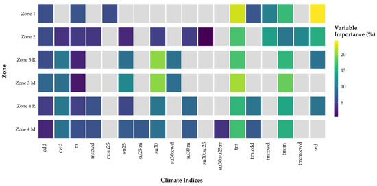
Figure 3.
Variable importance MLR model for each zone. All colored boxes represent variables that were used in each individual MLR model, variables that were not used are colored grey. The color gradient shows the variable importance for each zone; consecutive dry days (cdd), consecutive wet days (cwd), month (m), summer days (su25), hot days (su30), air temperature (tm) and days of the week (wd).
4.2.2. GMLR Model
To derive a GMLR model for the tool, the individual MLR models were compared with each other. It was found that some variables appeared in all models. To build this GMLR model, the variables that were found to be significant in at least four of the individual regression models were selected. With the selected variables, a GMLR model was derived for all study sites. The following variables were used to build the GMLR model:
- Mean temperature (tm);
- Hot days (su30);
- Summer days (su25);
- Days of the week (wd);
- Month (m);
- Consecutive dry days (cdd);
- Consecutive wet days (cwd);
- Combination of mean temperature and month (tm:m).
Figure 4 shows the variable importance for the GMLR model in each zone. The variable mean air temperature was one of the most important variables in all zones. In Zone 1, besides the mean temperature, the variable days of the week and the combination of mean temperature and month were very important. In Zone 2 the heat parameters, like summer and hot days were the least important. This may be related to the fact that the zone was composed of both residential and industrial use. Zone 3 R and Zone 3 M did not differ much, here the climate indices hot days, mean air temperature and the combination were evaluated as most important. The main difference between Zone 4 R and Zone 4 M was that the days of the week had less influence in Zone 4 M. This can be attributed to the data preparation since the rolling mean not only smooths the pumping peaks but also blurs the days of the week together.
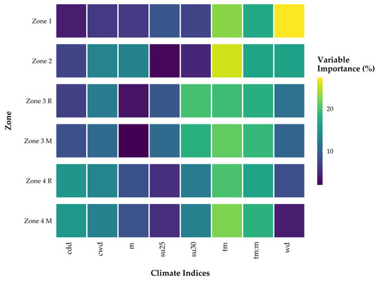
Figure 4.
Variable importance GMLR model for each zone. The color gradations represent the variable importance of the GMLR model of each zone. The brighter the box the more important is the variable in the corresponding zone; consecutive dry days (cdd), consecutive wet days (cwd), month (m), summer days (su25), hot days (su30), air temperature (tm) and days of the week (wd).
4.2.3. Model Training, Testing and Evaluation
For training the SVR, RF and ANN models, the training data set including the variables days of the week and month in the form of a binary class matrix was used. The model accuracy of all models (MLR, GMLR, SVR, RF and ANN) was quantified with the metrics introduced in Section 3.2.6.
To check if the GMLR model achieves similar results to the other applied models, the results from the model accuracy test were compared between the applied models.
Table 2 shows the results from the model accuracy tests. The GMLR model achieved good model accuracy for all zones. The best results were achieved for Zone 1, where the MAPE was only 5% by average between the predicted demand and the measured. For each zone, a good model accuracy with a low MAPE was achieved.
Table 2.
Model accuracy for the training data set (2017–2018) for all applied modeling approaches. The results from the GMLR model are highlighted in bold letters.
It can be seen that the MAPE of the applied models did not differ significantly within the individual zones. The correlation differed significantly between models and zones. The GMLR model provided almost similar results to the individual MLR models in terms of model accuracy tests. The RMSE and MAE results could not be compared across all zones, as they depended on the system water capacity. None of the models clearly outperformed another.
After training the models, the daily water demand was predicted using the test data set. As with the training data set, the model accuracy was determined for each modeling approach and then checked to see how the GMLR model performed in comparison to the other modeling approaches. In Table 3 the model accuracy for the test data set for each applied model is shown. The results were similar to those received with the training data set. The GMLR model performed similarly compared to the other models with respect to MAPE. Between models and zones, the correlation differed significantly. RMSE and MAE also differed between the zones, but the difference was within an acceptable range. The GMLR model offered acceptable performance for the task compared to the individual MLR models.
Table 3.
Model accuracy for the test data set (2019) for all applied modeling approaches. The results from the GMLR model are highlighted in bold.
4.3. Short-Term Peak Water Demand Days Evaluation
The next step is to check whether the GMLR model can predict the number of peak water demand days with sufficient accuracy. The water demand was predicted with the GMLR model for the time period 2017–2019 with the climate indices calculated from the weather records. Further, the number of peak water demand days (upper 10% range of demand) was determined and then compared with the number of peak water demand days from the water demand records. In Table 4 the mean number of peak water demand days per year predicted with the GMLR model and the water demand records were compared. It is shown that the difference was only a few days.
Table 4.
Comparison of the mean number of peak water demand days per year between the results from weather data and the water demand records, for the time period 2017–2019.
The GMLR model slightly overestimated the number of peak water demand days. Nevertheless, the deviation was in an acceptable range. The years 2017–2019 are among the hottest years in Austria’s weather measurement history [32], this could be the reason why the GMLR model overestimated the number of peak water demand days. Given the short time series and the variability of the weather records, the GMLR model provided satisfactory results.
For the future water demand forecast, which was undertaken next, for Zone 3 and 4 only the smoothed data (Zone 3 M and Zone 4 M) were used.
4.4. Long-Term Peak Water Demand Estimation
Since climate change depends on several factors, it is not possible to make a precise statement about how the climate will behave in the future. The climate projections represent only one of the possible future climate change scenarios. Nevertheless, we could use these projections to estimate a range of possible future water demands.
To use the appropriate climate projections for the two supply areas Vienna and Graz, the closest gridbox was chosen for the supply system. Furthermore, it is assumed that in both zones there are no major demographic developments in the selected time period. To be able to make a valid statement, a long time period must be chosen to cover the year to year climate variability. Therefore, the climate projections were split up into a reference period from 1980 to 2005 and a future period from 2025 to 2050. The historical period 1980–2005 was chosen as a suitable comparable reference period, as the short-term period (2017–2019) was not significant enough. For this forecast, 16 different climate projections representing the RCP8.5 were available and used. For each of the 16 climate projections the future water demand was projected using the GMLR model. This results in a range of possible water demands for each zone.
In a first step, we evaluated the change in the climate indices. Figure 5 shows the climate indices for the reference (1980–2005) and the future period (2025–2050) for Vienna and Graz. An increase in mean air temperature for Vienna and Graz is noticeable. Additionally, an increase can be seen in the number of hot and summer days. The number of consecutive dry and consecutive wet days would remain very similar for this scenario, compared to the reference period. A significant increase in heat waves was recorded for Vienna and Graz. Furthermore, we compared the maximum temperature of the reference period with the maximum temperature for the future forecasts and there was a temperature increase of 1.7 °C in Vienna and 1.6 °C in Graz. Comparing the results with the projections from the ÖKS 15 study [17], it can be seen that the increase in mean air temperature and summer days were approximately the same.
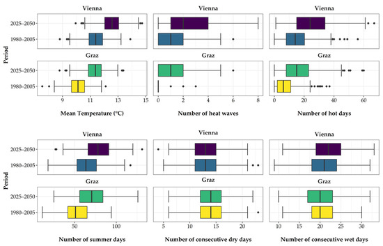
Figure 5.
Comparison of the climate indices for the time period 2025–2050 with the reference period 1980–2005 for Graz and Vienna. In this figure the bandwidth of climate indices is shown resulting from 16 different climate projections.
With the GMLR model, the water demand was estimated for the 16 available climate projections for both selected periods. We compared the peak water demand from the climate projections for 1980–2005 with the peak water demand for the time period 2025–2050. We calculated the percentage change between the peak water demand 1980–2005 and the peak water demand for the future time period 2025–2050 (Figure 6). The change of the peak water demand was given in a range. This range resulted from the individual forecasts for the 16 climate projections. As can be seen in Figure 6, peak water demand was projected to increase for most climate projections, but for some climate projections the GMLR model projected a decrease in peak water demand. This may be due to the different changes in the climate indices in the individual climate projections.
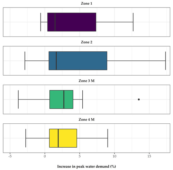
Figure 6.
Increase in peak water demand. The percentage change of future peak water demand is shown in relation to the reference period.
Furthermore, the average change in peak water demand was determined. For Zone 1 an average increase in peak water demand of 3.9% was found. The peak water demand in Zone 2 will increase by 5.1% on average. For Zones 3 M and Zone 4 M it was found that the peak water demand was expected to increase by 2.5% on average. On average, this resulted in an increase in future peak water demand for the climate classification cfb of 3.5%.
Furthermore, the future peak water demand days were determined, these are shown in Figure 7. The left side shows the number of peak water demand days for the reference period 1980–2005 and the right side shows the number of peak water demand days for the period 2025–2050. While the average of all projections shows a slight increase of 1 peak water demand day, there were some projections that project a decrease. This was again due to the previously mentioned different changes of the climate projections.
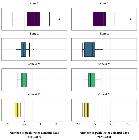
Figure 7.
Number of peak water demand days. The left side shows the number of peak water demand days for the reference period (1980–2005). The right side shows the number of peak water demand days for the time period 2025–2050. The bandwidth of the depicted values results from 16 different climate projections.
From these results shown above, it can be concluded that the GMLR model provides satisfactory and reasonable results. The GMLR model represents the increase of the water demand in relation to the increase of the temperature-based climate indices appropriately. Which suggests that the derived model can be applied to the selected study sites.
5. Conclusions
The presented GMLR model predicted the daily water demand by incorporating climate indices derived from historical weather records or climate projections and parameters with respect to the seasonality of the water demand like days of the week and month. To evaluate, whether the developed GMLR model delivered reasonable results, model accuracy tests were undertaken using Pearson correlation or MAPE with training and testing data. Besides that, the modeling results were compared with results from different applied modeling approaches, like MLR, SVR, ANN or RF. The results showed that for the investigated supply zones, all models provided satisfying and similar results. For the time period 2017–2019 the number of peak water demand days could be predicted with acceptable accuracy with the derived GMLR.
Therefore, in a next step, the peak water demand and peak water demand days for the period 1980–2005 and 2025–2050 was estimated using the GMLR model and climate indices derived from 16 climate projections. The use of the model with the climate projections showed an increase in the temperature-based climate indices for the period 2025–2050, which also results in an increase in peak water demand. For the climate classification cfb an average increase in a peak water demand of 3.5% was estimated in relation to the reference period 1980–2005. Further, a mean increase of one peak water demand day can be expected for the worst-case climate change scenario for the time period 2025–2050. Hence, the application of the GMLR model could confirm the expected increase in peak water demand for the investigated supply zones.
When compared with the results from the study of Vonk et al. [10], where an average increase of the peak water demand of 6.5% by 2050 was estimated compared to the reference period (1995–2010), using eight scenarios that are based on RCP4.5, RCP6.0 and RCP8.5. Additionally, compared with a study from Toronto [8], where a peak water demand increase of 1.8% was predicted compared to the year 2000, resulting from a maximum temperature increase of 1 °C, our results were within a similar range. With the presented GMLR we estimated an average increase in peak water demand of 3.5% resulting from an average maximum temperature increase of 1.65 °C in the investigated study sites.
The annual variability of water demand caused by the variability of weather and climate was better represented with a longer time series, which allows one to reduce the uncertainties that arise from this variability. For our purpose, the model gave satisfying results for estimating the future peak water demand and peak water demand days. Nevertheless, with a longer time series for training and testing, the modeling approach is expected to perform better, e.g., in estimating the effects of dry and hot weather periods on garden irrigation or pool fillings, which is not regulated so far in Austria.
In addition, to improve the model performance, demographic development will be considered in the next step. To represent a broader range of climate change, additional future time periods and other climate change scenarios will be considered.
Author Contributions
Conceptualization, A.S. and D.F.-H.; methodology, A.S. and M.P.; validation, A.S.; formal analysis, A.S.; investigation, A.S.; resources, D.F.-H.; data curation, A.S. and M.P.; writing—original draft preparation, A.S. and D.F-H; writing—review and editing, A.S., M.P. and D.F.-H.; visualization, A.S. and M.P.; supervision, D.F.-H.; project administration, D.F.-H.; funding acquisition, D.F.-H. All authors have read and agreed to the published version of the manuscript.
Funding
This research is part of the research project EWA funded by the Federal Ministry of Agriculture, Regions and Tourism. https://www.bmlrt.gv.at/wasser/foerderungen/projektstart-wasserversorgung.html [12] (accessed on 14 June 2021). Open Access Funding by Graz University of Technology.
Institutional Review Board Statement
Not applicable.
Informed Consent Statement
Not applicable.
Data Availability Statement
The data presented in this study are available on request from the corresponding author.
Acknowledgments
We sincerely like to thank Municipal Department 31-Vienna Water and Holding Graz for sharing their zonal inflow data. We would like to thank Roman Maier [14] for providing the precipitation records. Further, we would like to thank Mag. rer. nat. Heimo Truhetz from Wegener Center for Climate and Global Change [17] for the detailed discussions on climate projections. We are grateful for the helpful and constructive review comments that helped to improve this work significantly. Therefore, we would also like to thank the reviewers.
Conflicts of Interest
The authors declare no conflict of interest. The funders had no role in the design of the study; in the collection, analyses, or interpretation of data; in the writing of the manuscript, or in the decision to publish the results.
References
- Murdock, S.H.; Albrecht, D.E.; Hamm, R.R.; Backman, K. Role of Sociodemographic Characteristics in Projections of Water Use. J. Water Resour. Plan. Manag. 1991, 117, 235–251. [Google Scholar] [CrossRef]
- Wang, X.; Zhang, J.; Shahid, S.; Guan, E.; Wu, Y.; Gao, J.; He, R. Adaptation to Climate Change Impacts on Water Demand. Mitig. Adapt. Strateg. Glob. Chang. 2016, 21, 81–99. [Google Scholar] [CrossRef]
- Amt der Oö. Landesregierung, Direktion Umwelt und Wasserwirtschaft; Abteilung Wasserwirtschaft, Wasserversorgung in Oberösterreich: Situationsbericht, geplante Maßnahmen und Empfehlungen gegen Auswirkungen des Klimawandels. Available online: https://www.land-oberoesterreich.gv.at/Mediendateien/Formulare/Dokumente%20UWD%20Abt_WW/2019_Trockenheit_und_Wasserversorgung.pdf (accessed on 8 July 2021).
- Donkor, E.A.; Mazzuchi, T.A.; Soyer, R.; Alan Roberson, J. Urban Water Demand Forecasting: Review of Methods and Models. J. Water Resour. Plan. Manag. 2014, 140, 146–159. [Google Scholar] [CrossRef]
- Vijai, P.; Bagavathi Sivakumar, P. Performance Comparison of Techniques for Water Demand Forecasting. Procedia Comput. Sci. 2018, 143, 258–266. [Google Scholar] [CrossRef]
- Msiza, I.; Nelwamondo, F.; Marwala, T. Water Demand Prediction Using Artificial Neural Networks and Support Vector Regression. J. Comput. 2008, 3. [Google Scholar] [CrossRef]
- Zubaidi, S.L.; Ortega-Martorell, S.; Kot, P.; Alkhaddar, R.M.; Abdellatif, M.; Gharghan, S.K.; Ahmed, M.S.; Hashim, K. A Method for Predicting Long-Term Municipal Water Demands Under Climate Change. Water Resour. Manag. 2020, 34, 1265–1279. [Google Scholar] [CrossRef]
- Sadiq, W.; Karney, B. Modeling Water Demand Considering Impact of Climate Change—A Toronto Case Study. J. Water Manag. Model. 2004. [Google Scholar] [CrossRef][Green Version]
- Donevska, K.; Panov, A. Climate Change Impact on Water Supply Demands: Case Study of the City of Skopje. Water Supply 2019, 19, 2172–2178. [Google Scholar] [CrossRef]
- Vonk, E.; Cirkel, D.G.; Blokker, M. Estimating Peak Daily Water Demand under Different Climate Change and Vacation Scenarios. Water 2019, 11, 1874. [Google Scholar] [CrossRef]
- Neunteufel, R.; Richard, L.; Perfler, R.; Tuschel, S.; Mader, K.; Haas, E. Wasserverbrauch und Wasserbedarf-Auswertung empirischer Daten zum Wasserverbrauch. Bundesministerium für Land- und Forstwirtschaft, Umwelt und Wasserwirtschaft, 2012, Wien, 252. Available online: http://docplayer.org/7566410-Wasserverbrauch-und-wasserbedarf-auswertung-empirischer-daten-zum-wasserverbrauch.html (accessed on 8 July 2021).
- bmlrt Projektstart zu EWA—Entscheidungsfindung in der WAsserversorgung unter Berücksichtigung von Wandel. Available online: https://www.bmlrt.gv.at/wasser/foerderungen/projektstart-wasserversorgung.html (accessed on 27 April 2021).
- Central Institute for Meteorology and Geodynamics (ZAMG). Jahrbuch—ZAMG. Available online: https://www.zamg.ac.at/cms/de/klima/klimauebersichten/jahrbuch (accessed on 30 April 2021).
- Maier, R.; Krebs, G.; Pichler, M.; Muschalla, D.; Gruber, G. Spatial Rainfall Variability in Urban Environments—High-Density Precipitation Measurements on a City-Scale. Water 2020, 12, 1157. [Google Scholar] [CrossRef]
- Moss, R.H.; Edmonds, J.A.; Hibbard, K.A.; Manning, M.R.; Rose, S.K.; van Vuuren, D.P.; Carter, T.R.; Emori, S.; Kainuma, M.; Kram, T.; et al. The next Generation of Scenarios for Climate Change Research and Assessment. Nature 2010, 463, 747–756. [Google Scholar] [CrossRef] [PubMed]
- Van Vuuren, D.P.; Edmonds, J.; Kainuma, M.; Riahi, K.; Thomson, A.; Hibbard, K.; Hurtt, G.C.; Kram, T.; Krey, V.; Lamarque, J.-F.; et al. The Representative Concentration Pathways: An Overview. Clim. Chang. 2011, 109, 5. [Google Scholar] [CrossRef]
- Chimani, B.; Heinrich, G.; Hofstätter, M.; Kerschbaumer, M.; Kienberger, S.; Leuprecht, A.; Lexer, A.; Peßenteiner, S.; Poetsch, M.S.; Salzmann, M.; et al. Endbericht ÖKS15—Klimaszenarien Für Österreich—Daten—Methoden—Klimaanalyse—CCCA Data Server. Available online: https://data.ccca.ac.at/dataset/endbericht-oks15-klimaszenarien-fur-osterreich-daten-methoden-klimaanalyse-v01 (accessed on 18 March 2021).
- CCCA Data Server. Available online: https://data.ccca.ac.at/ (accessed on 30 April 2021).
- Rubel, F.; Brugger, K.; Haslinger, K.; Auer, I. The Climate of the European Alps: Shift of Very High Resolution Köppen-Geiger Climate Zones 1800–2100. Meteorol. Z. 2017, 26, 115–125. [Google Scholar] [CrossRef]
- Adamowski, J. Peak Daily Water Demand Forecast Modeling Using Artificial Neural Networks. J. Water Resour. Plan. Manag. 2008, 134. [Google Scholar] [CrossRef]
- Adamowski, J.; Chan, H.; Prasher, S.; Ozga-Zielinski, B.; Sliusarieva, A. Comparison of Multiple Linear and Nonlinear Regression, Autoregressive Integrated Moving Average, Artificial Neural Network, and Wavelet Artificial Neural Network Methods for Urban Water Demand Forecasting in Montreal, Canada. Water Resour. Res. 2012, 48, 1528. [Google Scholar] [CrossRef]
- Boser, B.; Guyon, I.; Vapnik, V. A Training Algorithm for Optimal Margin Classifier. In Proceedings of the Fifth Annual ACM Workshop on Computational Learning Theory, Pittsburgh, PA, USA, 27–29 July 1992; Volume 5. [Google Scholar] [CrossRef]
- Deng, N.; Tian, Y.; Zhang, C. Support Vector Machines: Optimization Based Theory, Algorithms, and Extensions, 1st ed.; Chapman and Hall/CRC: Boca Raton, FL, USA, 2013; ISBN 978-0-429-11028-3. [Google Scholar]
- Meyer, D.; Dimitriadou, E.; Hornik, K.; Weingessel, A.; Leisch, F. e1071: Misc Functions of the Department of Statistics, Probability Theory Group (Formerly: E1071), TU Wien. R Package Version 1.7-4. 2020. Available online: https://CRAN.R-project.org/package=e1071 (accessed on 8 July 2021).
- Sauer, S. Moderne Datenanalyse mit R: Daten Einlesen, Aufbereiten, Visualisieren, Modellieren und Kommunizieren; FOM-Edition; Springer Fachmedien Wiesbaden: Wiesbaden, Germany, 2019; ISBN 978-3-658-21586-6. [Google Scholar]
- Breiman, L. Random Forests. Mach. Learn. 2001, 45, 5–32. [Google Scholar] [CrossRef]
- Chen, G.; Long, T.; Xiong, J.; Bai, Y. Multiple Random Forests Modelling for Urban Water Consumption Forecasting. Water Resour. Manag. 2017, 31. [Google Scholar] [CrossRef]
- Liaw, A.; Wiener, M. Classification and Regression by RandomForest. R News 2002, 2, 18–22. [Google Scholar]
- Allaire, J.J.; Chollet, F. keras: R Interface to ’Keras’. R Package Version 2.3.0.0. 2020. Available online: https://CRAN.R-project.org/package=keras (accessed on 8 July 2021).
- Allaire, J.J.; Tang, Y. tensorflow: R Interface to ’TensorFlow’. R Package Version 2.2.0. 2020. Available online: https://CRAN.R-project.org/package=tensorflow (accessed on 8 July 2021).
- Gedefaw, M.; Hao, W.; Denghua, Y.; Girma, A. Variable Selection Methods for Water Demand Forecasting in Ethiopia: Case Study Gondar Town. Cogent Environ. Sci. 2018, 4, 1537067. [Google Scholar] [CrossRef]
- Central Institute for Meteorology and Geodynamics (ZAMG). Einer Der Heißesten Sommer Der Messgeschichte—ZAMG. Available online: https://www.zamg.ac.at/cms/de/klima/news/einer-der-heissesten-sommer-der-messgeschichte (accessed on 30 April 2021).
Publisher’s Note: MDPI stays neutral with regard to jurisdictional claims in published maps and institutional affiliations. |
© 2021 by the authors. Licensee MDPI, Basel, Switzerland. This article is an open access article distributed under the terms and conditions of the Creative Commons Attribution (CC BY) license (https://creativecommons.org/licenses/by/4.0/).