Article

Efficiency Assessment for Rehabilitated Francis Turbines Using URANS Simulations

Département de Génie Mécanique, École de Technologie Supérieure, Montréal, 1100 rue Notre Dame Ouest, Montreal, QC H3C 1K3, Canada
*
Author to whom correspondence should be addressed.
Water 2021, 13(14), 1883; https://doi.org/10.3390/w13141883
Submission received: 16 May 2021 / Revised: 27 June 2021 / Accepted: 30 June 2021 / Published: 7 July 2021
(This article belongs to the Special Issue Advances and Challenges in Hydropower)

Abstract

:
Due to the large number of aging hydraulic turbines in North America, rehabilitation is a growing market as these turbines have low efficiency compared to modern ones. Computational Fluid Dynamics identifies components with poor hydraulic performance. The models often used in industry are based on individually analyzing the sub-components of a turbine instead of full turbine simulations due to computational and time limitations. An industrial case has shown that such analyses may lead to underestimating the efficiency increases by modifying the stay vane. The unsteady full turbine simulation proposes to simulate all components simultaneously to assess this efficiency augmentation due to stay vane rehabilitation. The developed simulation methodology is used to evaluate the efficiency increase and the flow of two rehabilitated turbines with stay vane modifications. Comparison with model tests shows the accuracy of the simulations. However, the methodology used shows imprecision in predicting the efficiency increase compared to model tests. Further works should consider the use of more complex flow modeling methods to measure the efficiency increase by the stay vane modifications.

1. Introduction

Hydroelectricity provides approximately 16.2% of the total energy consumed worldwide [1]. With more than 100 years of existence in North America, hydropower produces 60% of the electricity consumed in Canada and approximately 10% of the needs of the United States [2]. A large number of plants provide this electricity, and many of them must be rehabilitated to assure continued operation. Major maintenance of a turbine-generator often involves the replacement of the runner as well as hydraulic modifications and is an excellent opportunity to increase performance.
In the rehabilitation process of large hydro-plants, Computational Fluid Dynamics (CFD) is often used to assess the turbine efficiency of existing installations and to identify problematic components [3,4,5,6]. The most common methods use a domain decomposition approach where simulations are run individually for each component, due to limited computing resources [7,8,9,10,11]. However, assumptions and simplifications of the flow are made when transmitting boundary conditions from one component to the other. Complete turbine simulation could assess efficiency more accurately, as it represents the flow with fewer assumptions and simplifications [12].
This large-scale computational approach has been made more accessible in research studies and has been used more and more frequently in industry, thanks to the increases in computing power [12,13,14]. A literature review shows that complete turbine simulations in modern geometries, without flow separations in the stay vanes (SVs), assess performance adequately at the best operating point (BEP) with the steady and unsteady Reynolds Averaged Navier-Stokes equations [11,15,16,17,18,19,20]. Outside the BEP, unsteady simulations are required to improve efficiency prediction, but they are more often used to measure pressure fluctuations in the distributor, the runner, and the draft tube to evaluate dynamic loads [15,17,20,21]. Many standard two-equation turbulence closure models are used, but their influence seems to be negligible, as shown by detailed analyses [22]. Recent works reveal that efficiency evaluation outside the BEP remains very difficult to assess, as flow separations in the runner and draft tube are under-predicted [18].
Few studies have focused on hydraulic turbine rehabilitation with case studies of boundary layer separation at the SVs. Most works focus on increasing efficiency by runner modifications or the replacement of guide vanes (GVs) [3,4,5]. One rehabilitation study with complete turbine simulations achieved efficiency augmentation by minor modifications to the SVs and the GVs [11]. The study of the draft tube flow is usually the main topic devoted to turbine rehabilitation, as complex turbulent phenomena in the flow could significantly decrease efficiency near the BEP [23,24].
This paper pushes the CFD capabilities to the analysis of full-scale hydraulic turbines by the study of SV modifications on the efficiency augmentation of rehabilitated Francis hydraulic turbines using URANS simulations. Two rehabilitated hydraulic turbines of similar specific speeds (Nsq of 64.4 RPM and 69.2 RPM) are studied. The first objective is to compare the efficiency predictions of full-turbine Unsteady Reynold Navier-Stokes (URANS) simulations with experimental data. The second objective is to analyze in more detail the influence of SV efficiency increase on the distributor, the runner, and the draft tube flow.
The numerical methodology is presented in the next section. The main numerical ingredients for the CFD code are briefly outlined along with the computational domain and the boundary conditions. Grid scaling tests are performed on the spiral case and tandem cascade, runner, and draft tube sub-domains. A brief presentation of the model test’s development along with the main experimental results are given in Section 2. The results of the unsteady full turbine simulations are presented in Section 3, where the efficiency increases are compared with the experimental data.

2. Numerical Methodology

The numerical methodology of full turbine simulations is based on a comparative approach to assess the efficiency losses in all components, and the increase of turbine efficiency with SV modifications, as indicated in Figure 1, in the rehabilitation process of two hydraulic turbines. Modifications to the first case (case 1) and the extension in the second case (case 2) mainly reduce the boundary layer separation at the leading edges of the SVs.
Numerical simulations are performed on both cases at the model test geometry dimensions (DRunner = 350 mm). The full turbine computational domain is composed of three subdomains corresponding to the spiral case, the runner, and the draft tube. Two interfaces are used to connect the fixed and rotating subdomains, as shown in Figure 2.
The spiral case domain includes 24 SVs and 24 GVs. The runner domain includes a 17-blade Francis runner with a shroud and a hub. The draft tube domain consists of an elbow diffuser and begins at the runner outlet. A rectangular extension is added at its exit to promote solution convergence and to reduce the domain size [25]. Interface 1, between the spiral case and the runner, is positioned approximately halfway between the GV’s trailing edge and the runner blade’s leading edge. Interface 2, between the runner and the draft tube, is positioned at a fixed distance to the blade’s trailing edge. This gives the interface a conical configuration, designed to reduce the numerical diffusion on the draft tube vortex. Figure 3 provides a 3D view of the full turbine simulation domain.

2.1. Numerical Parameters

The Reynolds number of the flow is 5.1 × 10⁶ in case 1 and 4.8 × 10⁶ in case 2, at model test dimension. The turbulent flow is computed using the ANSYS CFX solver [26]. Unsteady Reynolds-Averaged Navier-Stokes (URANS) equations, the k-ω SST turbulence model, and transient rotor-stator interfaces are used to conduct complete turbine simulations [26,27,28]. This interface type actualizes flow information between rotating and stationary domains at each time step without averaging flow quantities, which allows the wakes of older SV geometries to be well-resolved at the runner inlet. URANS simulations also improve the modeling of vortex phenomena in the draft tube flow [25].
Reynolds-Averaged Navier-Stokes (RANS) equations and the k-ω SST turbulence model are utilized to model the flow in spiral case simulations in the absence of rotating components. In every simulation, k-ω SST equations are used to capture the boundary layer separation at the SV and in draft tubes ([8,18]). This turbulence model is commonly used in hydraulic turbines, as it is good for capturing flow separation [29].
Numerical errors and their propagation in the flow are limited with the use of the second-order temporal Euler scheme, spatial discretization and advection schemes. In addition, mesh refinements in areas of high flow gradient help to reduce numerical errors. The ANSYS CFX advection scheme is used with β = 1. This coefficient adds an anti-diffusive correction to the Upwind Difference scheme for a fully second-order advection discretization.
In unsteady simulations, the time step is selected to achieve a statistical convergence to model the interactions between SV wakes and the runner blades and to reduce numerical errors. Seven rotations at 2° per time step (~4.2 × 10⁻⁴ s) are performed, followed by one at 0.5° (~1.05 × 10⁻⁴ s) to obtain the final solution. This unsteady strategy obtains good statistical convergence of the main hydraulic turbine quantities relative to their average value. The initial solution to these simulations is obtained from a steady computation using frozen rotor interfaces and the high-resolution advection scheme. The time step of the last rotation is comparable to the value used for the numerical analysis of rotor-stator interaction and draft tube pressure fluctuations in Francis turbines ([18,28,30]).
The Courant-Friedrichs-Levy (CFL) number quantifies the stability of the discretization scheme and the reduction of numerical errors. ANSYS CFX defines the CFL number for a one-dimensional grid as Equation (1). The average CFL number ~0.23 measured at the runner outlet, a high-velocity area in the turbine, at the smallest time step 0.5° suggests satisfactory stability as well as a satisfactory reduction of numerical errors [26]. The average CFL number for the turbine components at this time step is always less than one, with a maximum of 0.88 in the runner sub-domain.
C F L = u Δ t Δ x
Refer to the notation section for the definition of variables in Equation (1). Three iterations are generally required so that the residual’s maximum is less than 10−4 at each time step. However, in some simulations, there may be very few cells (0.003% of the runner’s sub-domain volume) near the blade’s inlet, where convergence is not fully achieved even after three iterations. This is mostly due to the lack of control over tetrahedral cell quality, combined with the high-velocity gradients in this area.

2.2. Boundary Conditions

In all of the simulations, the turbine discharge was imposed at the inlet with a fully developed analytical turbulent velocity profile pipe flow [31]. An average zero static pressure condition is imposed at the outlet. These boundary conditions are numerically stable and commonly used in hydraulic turbine simulations ([18,26]). Turbulence intensity of 5% is imposed at the spiral case inlet. The imposed discharge corresponds to the values measured in the model tests. For the two cases studied, a GV opening (γ) sets the operating point, Table 1, with a corresponding discharge coefficient.

2.3. Evaluation of Turbine Parameters

The numerical hydraulic turbine head (Hn) was evaluated according to IEC 60193 [32], Equation (2), where static pressure is the average value measured by pressure probes at a spiral case inlet (P1) or at a draft tube outlet (P2). The kinetic energy was computed using the turbine discharge amount Q and the flow area at a spiral case inlet A1 or at a draft tube outlet A2.
H n = P 1 ρ g + Q / A 1 2 2 g + z 1 P 2 ρ g + Q / A 2 2 2 g + z 2
Figure 4 shows the pressure probes and surface positions for turbine head evaluation.
The head loss of each component was computed using inlet and outlet control surfaces, as shown in Figure 4. The energy at the spiral case inlet and the draft tube outlet was evaluated by following the IEC method. For the other control surfaces, the energy was evaluated as the flow average defined in Equation (3) with the local mass flow.
E = m ˙ p T o t a l m ˙ ρ g
The efficiency loss coefficient ( Δ ψ / φ 2 ) is used to express the energy loss in each component of the turbine. Equations (4) and (5) show this coefficient by the difference of the energy coefficient between the inlet and the outlet components and the flow coefficient.
Δ ψ = E   O u t l e t E   I n l e t Ω 2 D 2
φ = Q Ω D 3
The energy head is compute, Equation (6), with the mechanical runner torque from the numerical simulations.
H i = 2 π Ω T Q g
In unsteady simulation, the results are an arithmetic average of all of the flow components at each time step of the 0.5° runner rotation. Refer to the notation section for the definition of variables in Equations (2)–(6).

2.4. Mesh Generation

Hybrid tetrahedral meshes generated with Pointwise 17.0 R2 [33] are used for the spatial discretization of full turbine and spiral case simulation domains. Mesh quality, construction turnaround time, and the quality of the results support the use of this mesh type rather than hexahedral structured meshes [34].
For the full turbine simulation, the spiral case, runner, and draft tube subdomains were meshed independently and then glued to impose flux continuities at the non-matching interfaces, using the General Grid Interface Module (GGI).
To model boundary layer separation at the SVs of old geometries, the Y+ in all of the meshes was set to approximately 2.5 to take advantage of the wall-flow resolution of the k-ω SST turbulence model [29]. With this Y+, only a few cells are in the viscous sub-layer and a minimum of 20 cells are in the turbulent boundary layer when using a 1.2 expansion factor. The Y+ on the SVs of case 2 is ~1 due to their rounded leading edges. Indeed, the SV chamfered edge of case 1 sets the boundary layer separation point position. Meshing parameters impose a minimum of 20 and a maximum of 60 prismatic tetrahedral cell layers on the walls to provide a smooth transition to tetrahedral cells. The hydraulic profile’s thin edges, the draft tube pier noses, and the runner’s cone are all spatially discretized with ordered tetrahedral cells. The volume mesh size was controlled by approximating the surface-to-volume cell size factor. According to these criteria, the spiral case meshes and full turbine simulations are similar to those shown in Figure 5 in the SV and GV zones.
Figure 6 shows a sectional view in the meridian plane of the runner mesh. Mesh density in the runner is principally dictated by numerical stability. High flow gradients need a sufficient mesh density on the blade’s leading and trailing edges.
Figure 7 shows the mesh in the draft tube slightly upstream of the pier.

2.5. Grid Scaling Test

The grid convergence index (GCI) method was followed to assess numerical errors and grid convergence [35]. The analysis of grid independence with the grid convergence index (GCI) method in full turbine simulations is complex and requires significant computational resources. For this reason, the GCI method uses three smaller sub-domains (spiral case and tandem cascade, runner, and draft tube) of the full turbine simulation (Table 2 and Table 3).
Grid density variation is accomplished with refinements on the SV, GV, and flange surfaces. Cells are also added in the volumes around SVs and GVs. The Y+ is the same for all grids of the spiral case and tandem cascade; it provides a similar flow resolution on walls. Three different grid densities (1 for fine, 2 for medium, and 3 for coarse density) for each case and geometry are used in the spiral case. Fine mesh of case 1 old geometry spiral case use significantly more nodes than new geometry to capture the velocity gradient on the sharp edge of the SVs.
The domain utilized for the runner simulation is a periodic passage with one runner blade and one GV. The outlet of this domain is about 0.56RRunner below the runner. The flow imposed at the GV inlet is an average uniform flow with the SV’s outlet orientation.
The draft tube simulation uses a limited domain with an inlet about 0.56RRunner below the runner and the same outlet as the complete turbine simulation domain. The velocity and turbulence fields imposed at the inlet come from an average flow of one runner rotation of a complete turbine simulation of case 1’s new geometry.
Table 4 shows the uncertainties and the extrapolated values of the efficiency loss in the spiral case domain obtained by the GCI method.
This method begins by evaluating the ratio ( c 21 et ε 21 ) between the representative size of the two mesh densities members ( h ) and the efficiency loss in the spiral case domain ( ϕ ) evaluated by simulation, Equations (7) and (8), to obtain the approximate relative error, Equation (9), and the numerical uncertainty, Equation (10). The calculation of numerical uncertainty using the apparent order of the simulations (p), evaluated by an iterative method, allows extrapolating the results of simulations with a size of cells near zero.
c 21 = h 2 h 1
ε 21 = ϕ 1 ϕ 2
e a 21 = ϕ 1 ϕ 2 ϕ 1
G D C f i n e 21 = 1.25 e a 21 c 21 p 1
Refer to the notation section for the definition of variables in Equations (7)–(10). Numerical uncertainty (GCIfine21) is relatively small, with a maximum value of 0.1% and a minimum of 0.04% with finer meshes. The apparent order of the simulations varies between 11.4 and 21.2, with no possible values for case 2’s new SVs. Negative values of ε3221 reveal oscillatory convergence in three cases. These are due to the small difference in the efficiency loss between each mesh density. Oscillatory convergence could indicate a level of the mesh-independence of the efficiency losses, as mesh densities appear to be sufficient to model boundary layer separations and recirculation zones at SVs, or in their absence, in the new geometries. These results allow the use of the medium mesh density in the spiral case for the complete turbine simulation.
Table 5 presents the results obtained by the GCI method in the runner and the draft tube sub-domains. The finer mesh allows a flow resolution up to the viscous sub-layer on the wall of those components. The efficiency losses in the runner are evaluated with a numerical error of 3.6%, the energy head with an error of 6.3%, and the efficiency losses in the draft tube with an error of 6.3%. These GCI method results indicate the achievement of a stable convergence. Medium-density meshes are used in the runner and in the draft tube for the complete turbine simulation (Table 6).
These simulations have required approximately 200 h with 120 CPUs for their resolution.

2.6. Model Tests

Experimental tests of two cases were carried out in previous studies (unpublished for proprietary reasons). They provide experimental efficiency values for cases 1 and 2. The tests were made according to IEC 60193 [36] and IEC 60995 [32] standards. The tests showed that SV modifications lead to efficiency increases of 2.2% and 1.0% in cases 1 and 2, respectively, at the BEP (Figure 8).
The model tests evaluated efficiency with systematic and random uncertainties stemming from the accuracy of the equipment and the measurement methods. According to the IEC 60193 methodology, the efficiency uncertainty is ±0.0013 for case 1 and ±0.0014 for case 2 for the BEP at maximal efficiency.

3. Results

The numerical results of full turbine simulations are used to assess efficiency increase, in each component, due to SV modification compared to that measured in model tests in both cases studied.

3.1. Efficiency Increase

The results of numerical simulations for the case 1 and 2 turbines are presented in Table 7.
Full turbine simulations determine a total reduction of the efficiency loss coefficient of 0.240 in case 1. This is 65% of the total efficiency loss coefficient reduction measured in model tests. In case 2, the simulations indicate a total efficiency loss coefficient reduction of 0.044 or 40% of that measured in model tests. In both cases, the main source of efficiency increase is from the SV. The GVs are the second-largest source of the reduction of the efficiency loss coefficient. The efficiency loss coefficient in the case 1 runner counts for 10.6% of the total while a slight increase is calculated in case 2. The magnitude of the efficiency loss variations in the spiral case and the draft tube is very low, as they appear to be within the range of numerical uncertainty for both cases. The absence of variation in the efficiency losses in the spiral case is normal, as there are no modifications to this component. The efficiency losses in the spiral case come from the wall friction and the secondary flows, and these phenomena are not affected by the flow modification in the SVs. The variation of the efficiency losses in the draft tube is very small compared to the total increase measured in the model tests.

3.2. Tandem Cascade

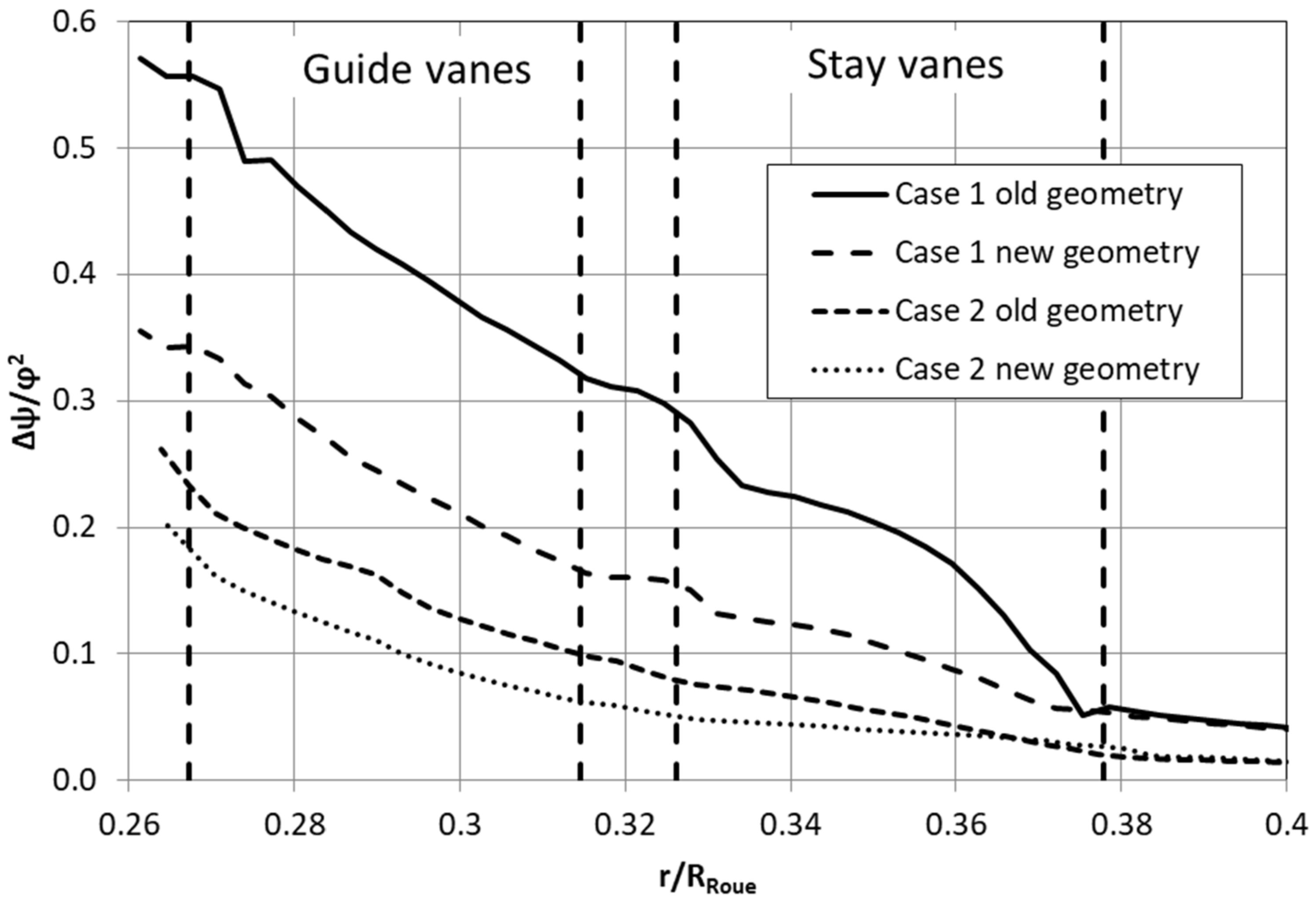
Figure 9 shows the efficiency loss coefficient as a function of the tandem cascade radius for the two cases studied. The comparison of the slope of the efficiency loss coefficient between the old and new geometries shows that in case 1, the main source of efficiency loss is located at the leading edge of the SVs. The other major efficiency losses are located at the exit of the old SVs in case 1. In the absence of new efficiency losses in the GVs, the slope is very similar between the two geometries for both cases.
In case 2, the difference in the slope of the efficiency loss coefficient between the two geometries is reduced relative to that of case 1. The slopes of the efficiency losses at the SVs of the old geometry are generally constant. They are only somewhat greater than those of the new SVs, and almost identical in the GVs. Similar to case 1, the increase is mostly generated in the SVs for both geometries.
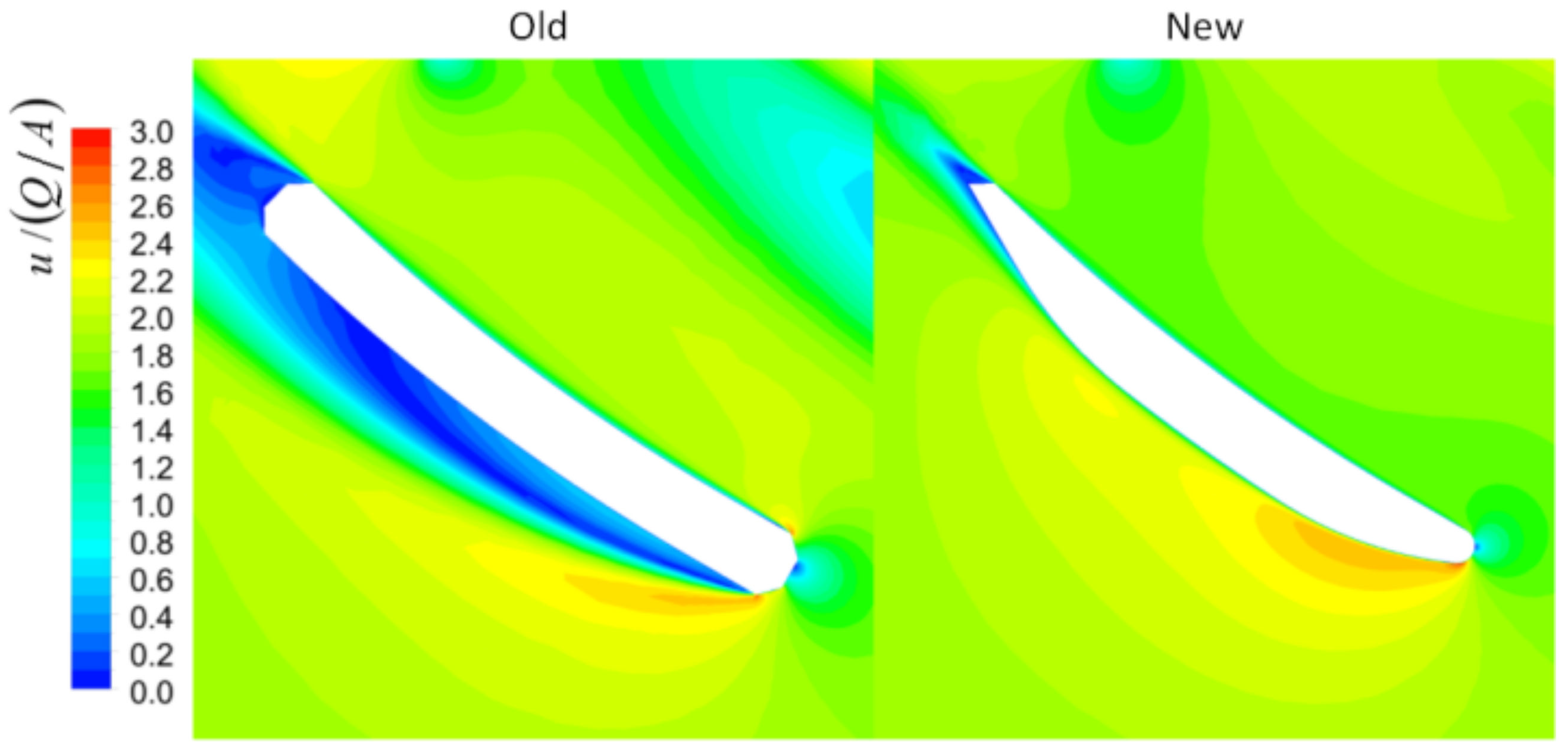
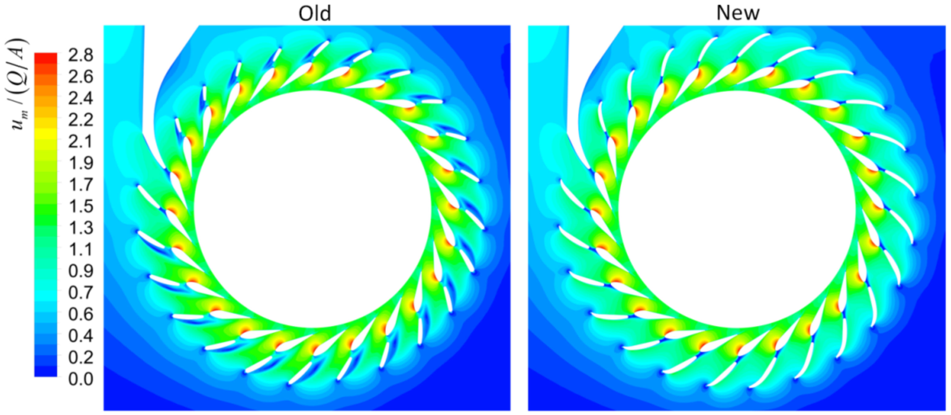
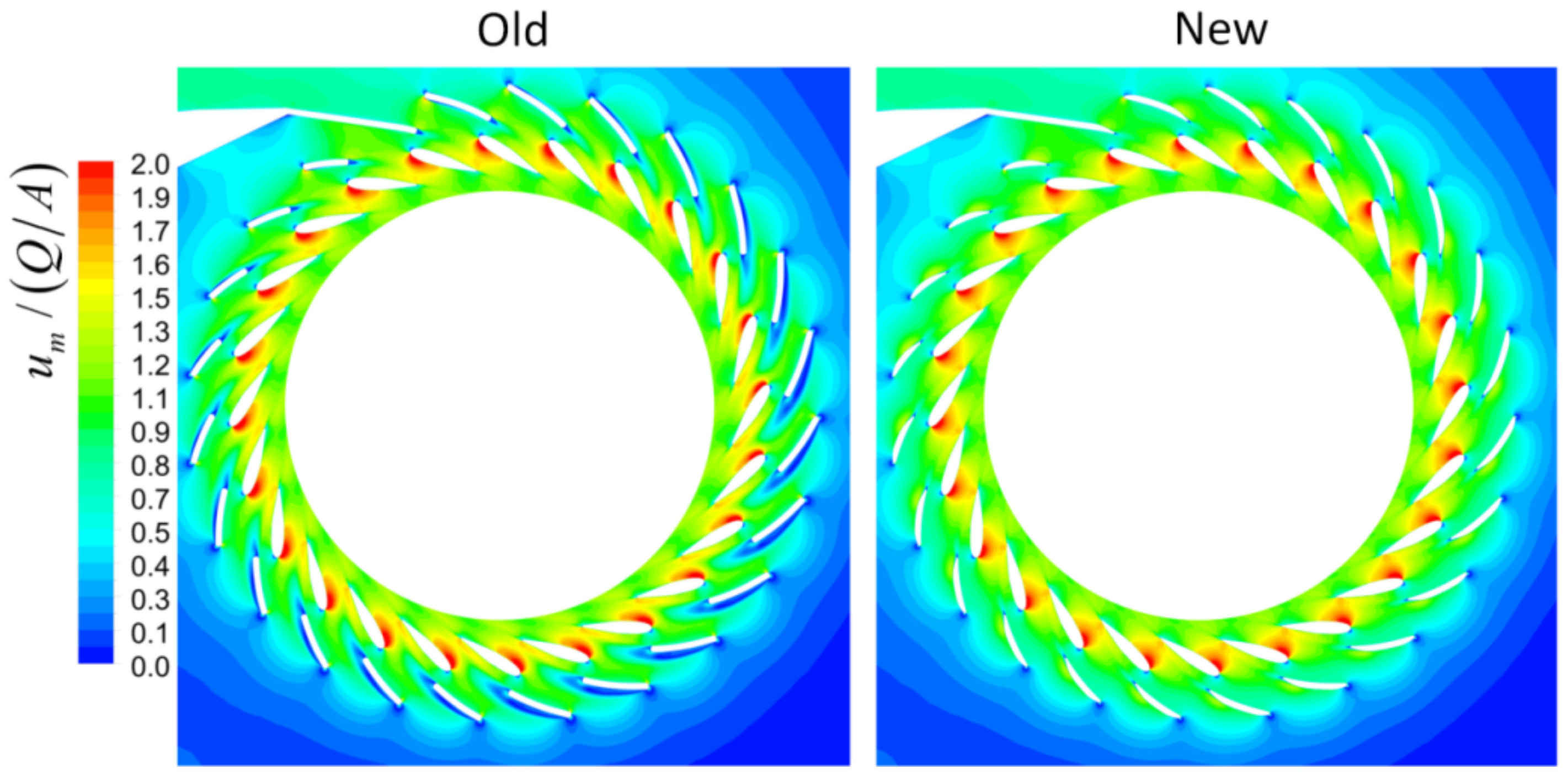
According to the observation of the efficiency loss coefficient in the tandem cascade, the significant reduction of efficiency losses is due to the elimination of the boundary layer separation at the SVs due to their modifications. The velocity at the SVs of the two geometries, Figure 10 and Figure 11, indicate the large boundary layer separation caused by the misalignment of their leading edges with the flow, as shown by the position of the stagnation point where the velocity is zero.
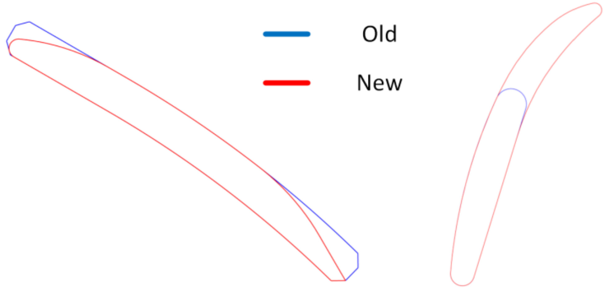
The flow misalignment is much more significant in the old geometry than in the new one, as the modification of the SVs significantly reduced the misalignment of their leading edges with the flow (see Table 8). This is the main cause of the recirculation zones and of the large efficiency losses in the old geometries of the two cases studied.
Added to the misalignment of the SVs to the flow, the velocity contours highlight the difficulty of a chamfer leading edge to keep the flow attached to the wall, as in case 1. Indeed, the velocity at the leading edge of the SVs reveals that the flow detaches from the wall on sharp chamfer angles due to the strong adverse pressure gradient created there. This is the boundary layer separation point and the beginning of the recirculation zone at the SVs. A boundary layer separation is also observed very locally on the SVs’ intrados. This separation shows the main weakness of chamfer geometry, as it creates efficiency losses even if the flow is properly oriented with the hydraulic profile. The modification to the SV’s geometry with a rounded leading edge attenuates this problem and reduces the incidence of flow misalignment, as evidenced by the velocity contour.
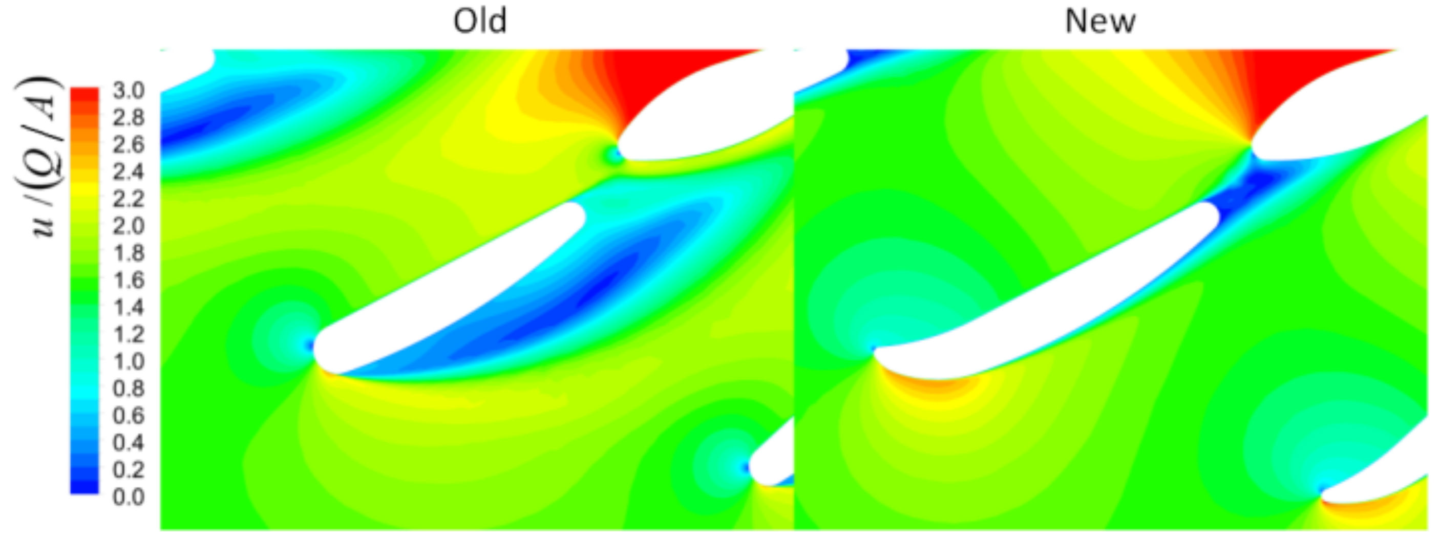
In case 2’s old geometry, the leading edges are appropriate to limit the boundary layer separation; however, the velocity contour shows the important misalignment of approximately 24° of the flow with the SVs. The increase in the adverse pressure gradient is due to the rapid change in direction of the SV’s leading edges. Indeed, this is the point of the boundary layer separation. By reducing the misalignment with the flow, the extension added to the new geometry attenuates the rapid change in direction of the SVs and therefore the magnitude of the adverse pressure gradient. However, the effect of a long application of adverse pressure gradient is observed on the upper surface of the SVs in the form of the flow slowing in the boundary layer. This slowing reveals the work of the SVs done on the flow to obtain an adequate orientation with the GVs.
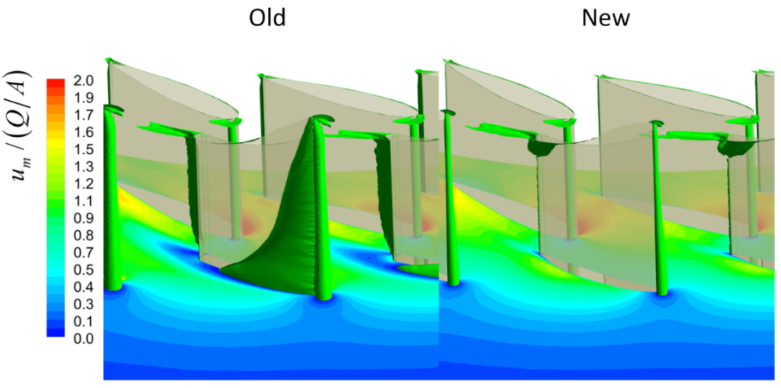
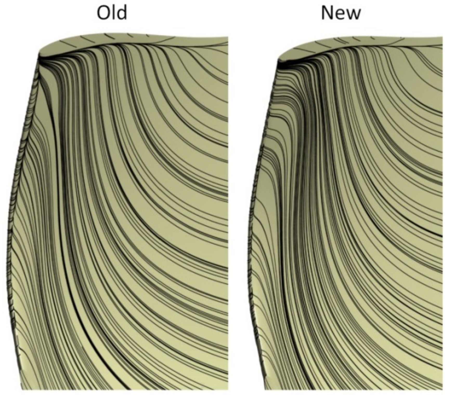
Flow observations at the tandem cascade show that the modification of the SVs eliminates all the recirculation zones (flow velocity almost zero) in the tandem cascade in both cases studied, as indicated in Figure 12 and Figure 13. In case 1, modification of the trailing edge of the SV also reduces its prominent wake. At the SVs located at the end of the spiral case with the small recirculation zone, a much larger wake is observed in the original geometry compared to the wake in the modified one. In both cases, the recirculation zones are closed in the GVs due to the flow restriction caused by the significant reduction of the flow section. This effect on the flow is visible through the zones of higher flow velocity at the entrance of the GVs.
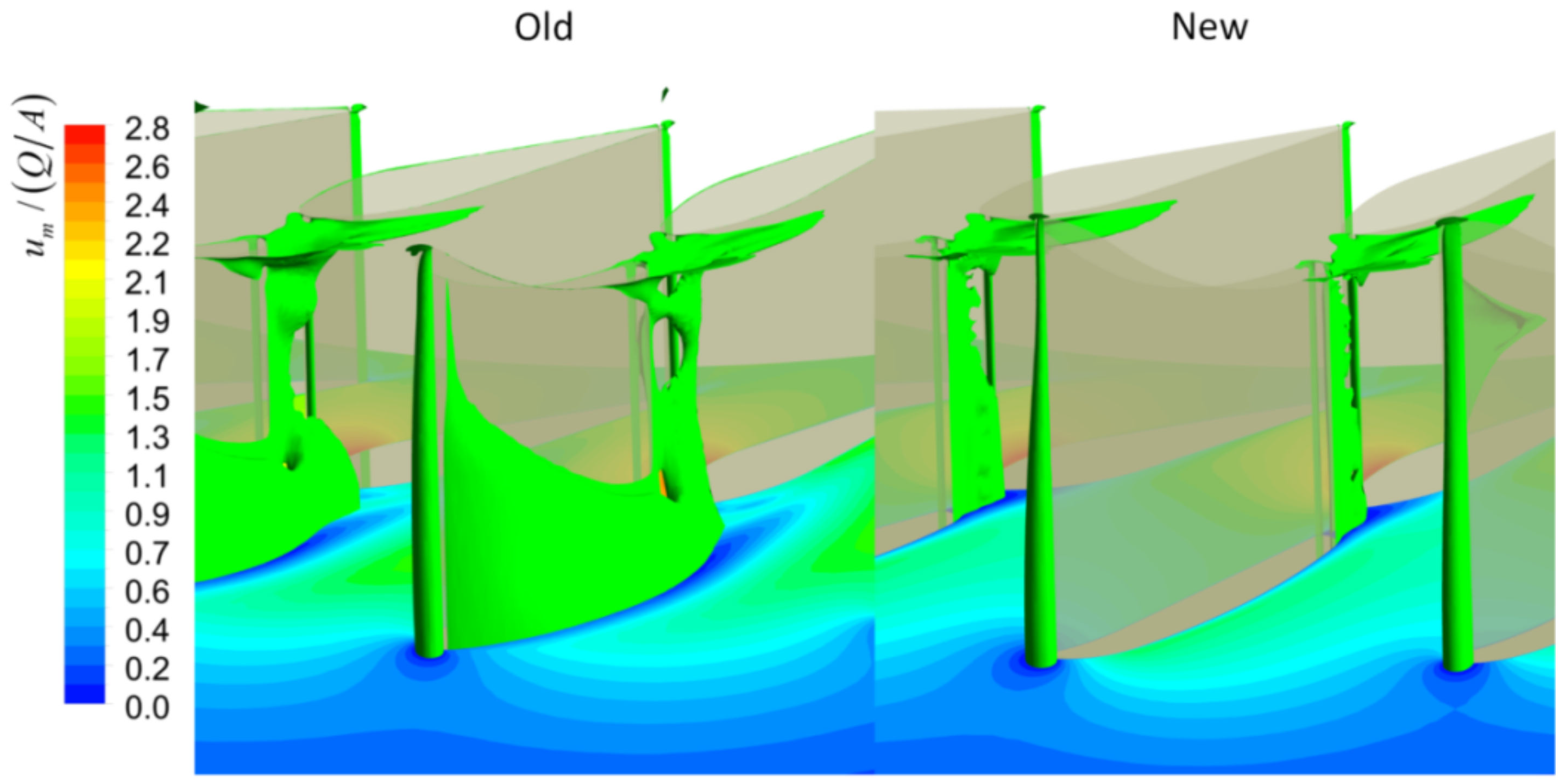
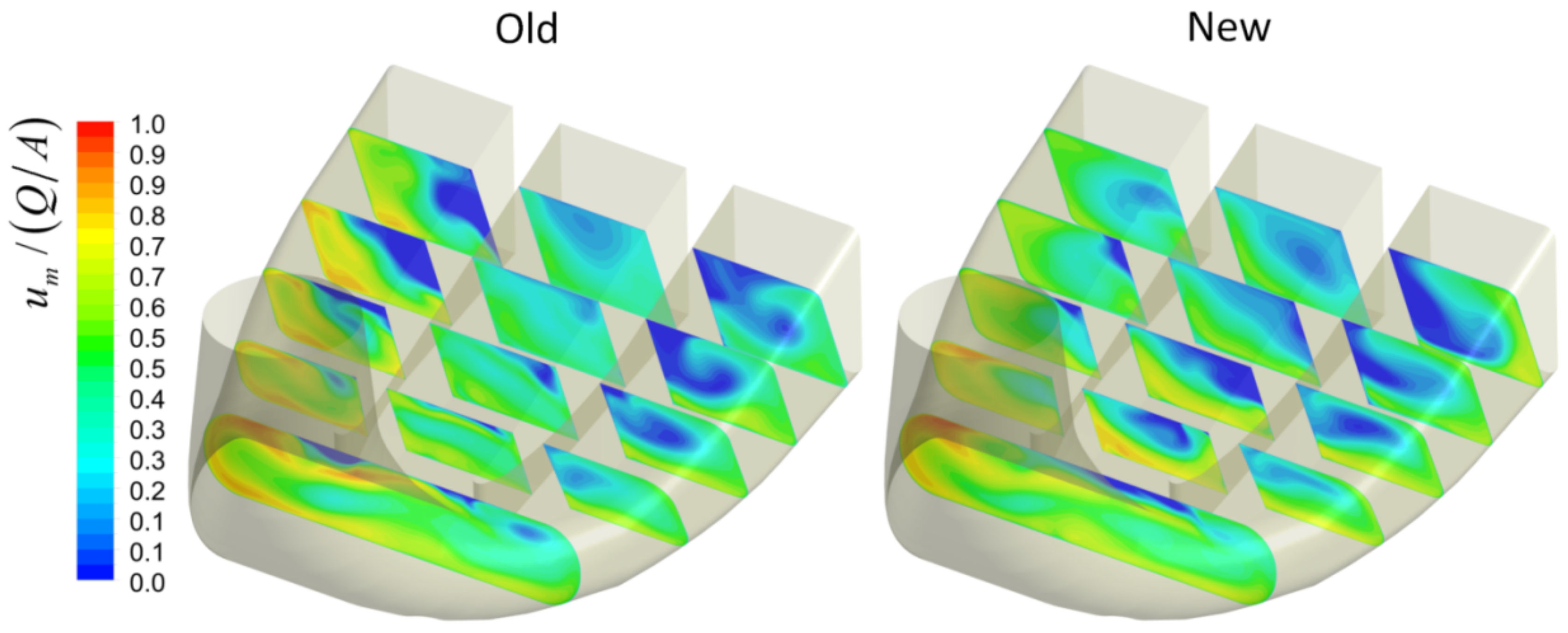
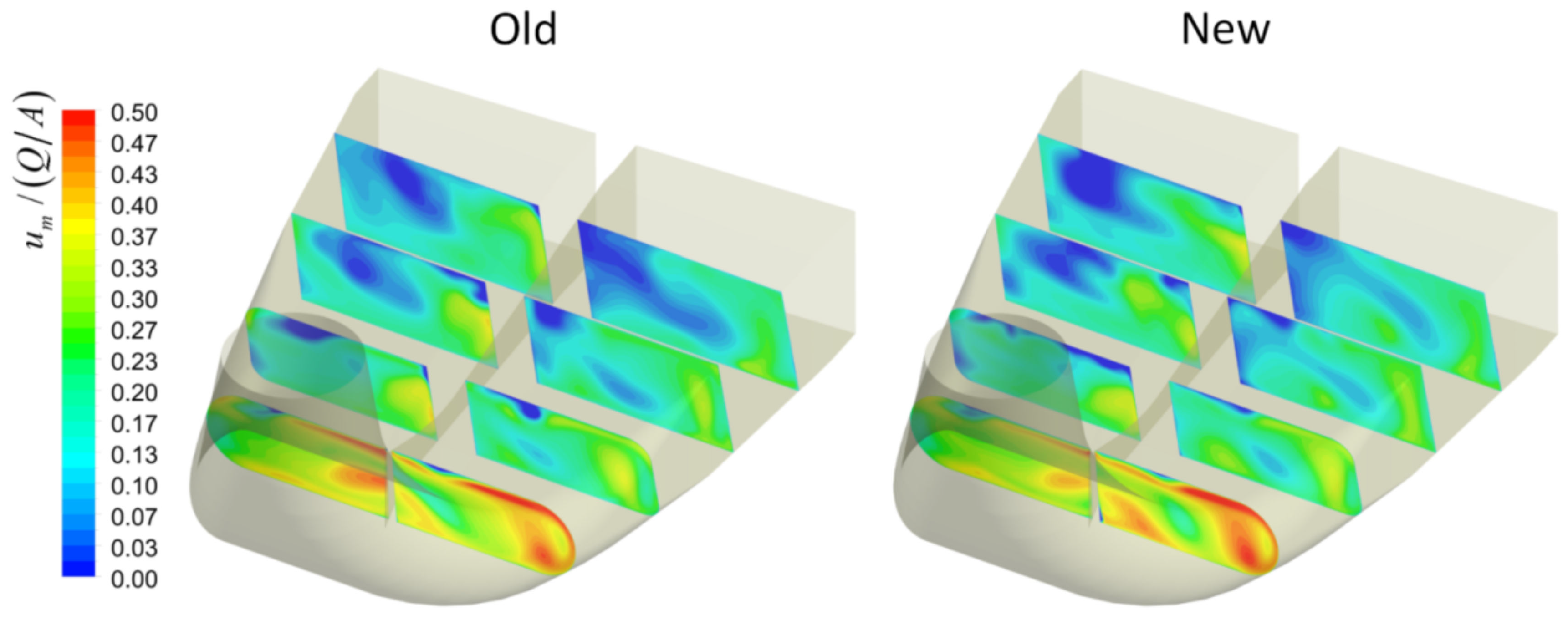
Figure 14 and Figure 15 show the large boundary layer separation in the old geometry with the recirculation zone highlighted by an isosurface of zero flow velocity (um = 0) and a contour of the flow velocity on the tandem cascade horizontal plane. Boundary layer separation is accentuated at the tandem cascade horizontal plane from the higher radial component of the flow at this location caused by the secondary flows in the spiral case. These figures show that the modification eliminates the boundary layer separation over the entire height of the SVs in the original geometry. However, the thinner trailing edge of the SV in case 1 adds a small recirculation zone near the flange, starting from the exit of the flange and the SV’s curve that lead to a local adverse pressure gradient increase.
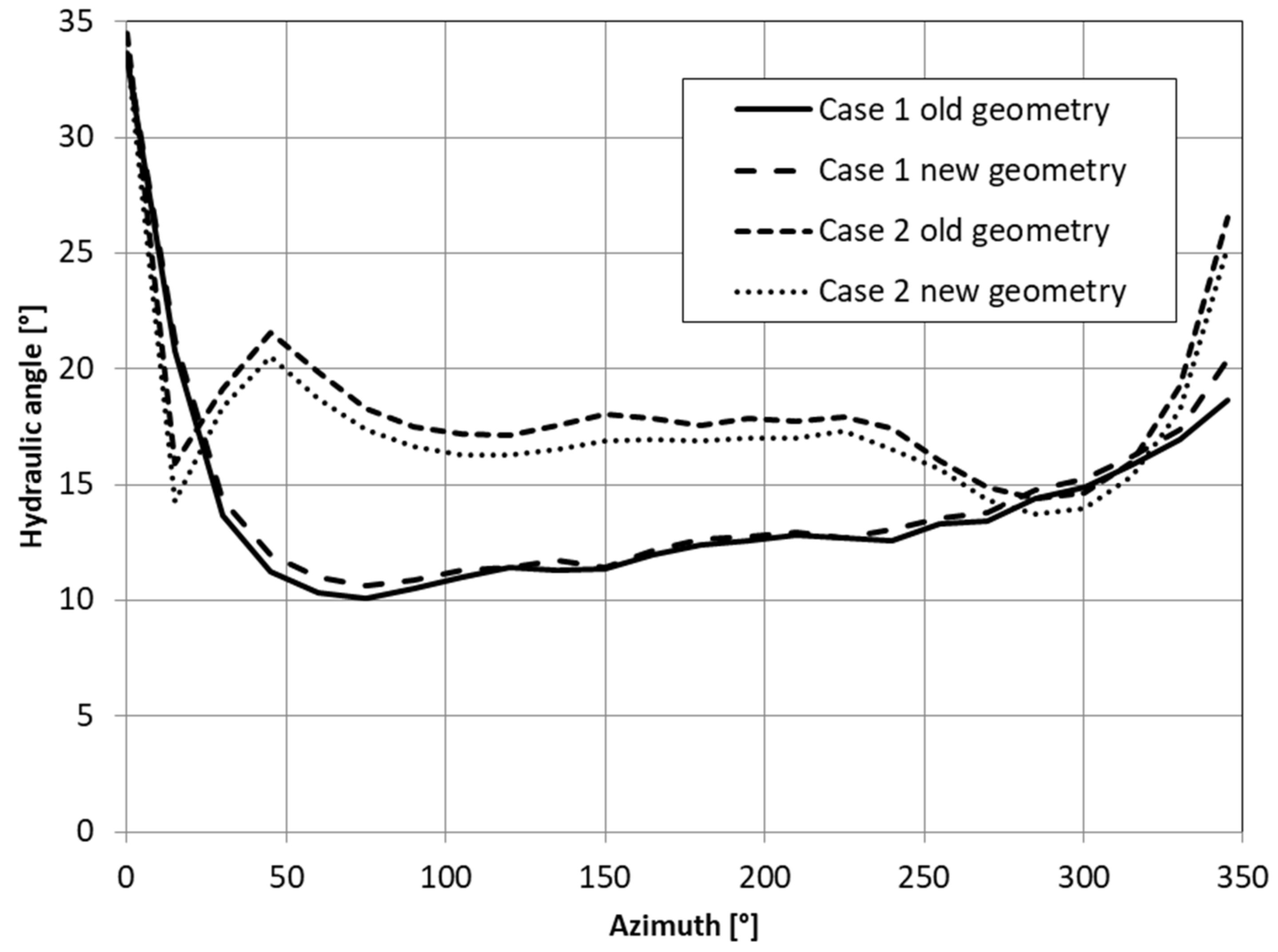
The azimuthal variation of the recirculation zones shows the variation of the flow direction at the leading edge of the SV. The spiral case imposes a more radial flow at its beginning and end while imposing a tangential direction to the flow in the middle, as shown in Figure 16. In both cases, the evolution of the azimuthal flow in the spiral case indicates this is a deceleration flow type; a result of the configuration of the spiral case [37]. This figure also shows, by its comparison between the old and new geometries, the absence of any influence of the recirculation zones on the flow direction at the SV’s leading edges.
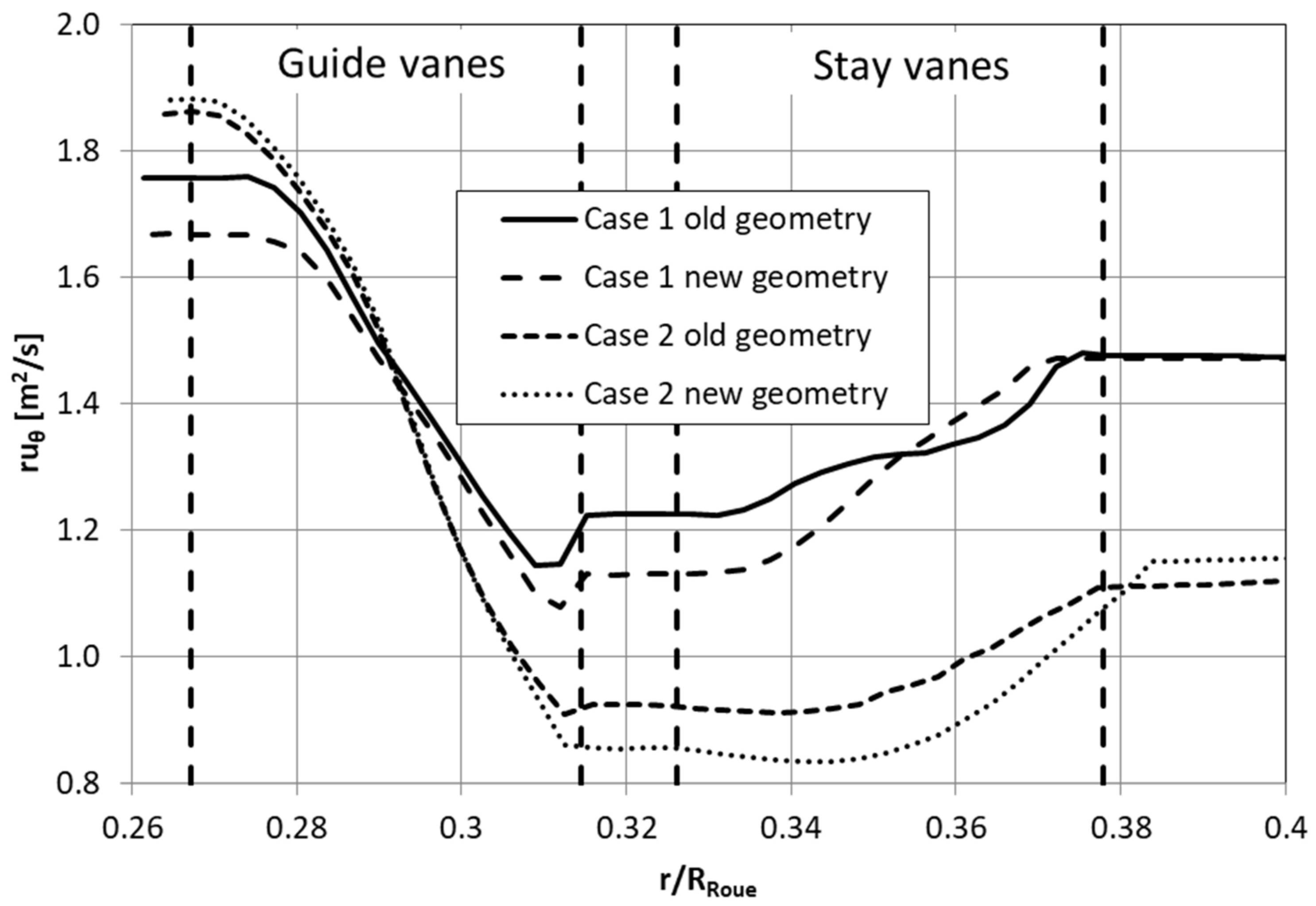
Recirculation zones in the tandem cascade affect the components of the mean flow at the exit of the GVs in the old geometry of case 1, as shown in Figure 17, with the angular momentum as a function of the radius. They have no effect on the angular momentum in the old geometry in case 2. Indeed, the recirculation zones in the original geometry increase the angular momentum provided to the GV’s outlet.
The effect of the recirculation zone can be noted at the boundary layer separation point on the leading edge of the SVs by a fast decrease in the angular momentum. The flow area reduction by the flow recirculation zones then increases the tangential component of the flow in the SVs. This result of a tangential flow at the exit of the SVs is significantly higher in the original geometry of case 1. For the old geometry, a similar effect is found in case 2 as the flow gains in angular momentum at the SV’s exit. In this case, it also appears that the recirculation zone partially blocks the radial component of the flow, thereby increasing the tangential flow. The comparison of the angular momentum at the exit of the GVs between the two geometries of case 2 shows that they restored the flow. However, in case 1, the old geometry maintains a higher angular momentum than the new one. This difference between the two geometries is due to the position of the SVs relative to the position of the guide vanes. The alignment of the GVs with the SVs in case 2 closes the recirculation zones and promotes the restoration of flow through the strong attenuation of the wake. On the contrary, in case 1, the position of the SVs between two GVs leads to the large wake of the recirculation zones at the exit of the GVs. This large wake creates a deficit of radial velocity with the effect of increasing the tangential flow, as at the exit of the SVs.

3.3. Runner

The efficiency loss variation between the old and new geometries in the case 1 runner is affected by the variation of the average flow component at the GV’s outlet. It is observed that the modification of the flow’s angular momentum by the recirculation zone in the old geometry implies a greater flow misalignment on the blade’s leading edge, as shown in Figure 18. In case 2, the absence of efficiency loss variation is the consequence of the very similar average flow component between the two geometries at the GV’s outlet.
Using the average velocity components, the hydraulic angle difference at a blade leading edge between the two geometries is about 0.35°. In contrast, the variation of the angle between the partial and the high load operation points is about 3°. If the flow misalignment is greater than that of the old geometry, it remains attached to the wall of the blade as shown by the streamline, with an increase of the energy runner head and efficiency losses.
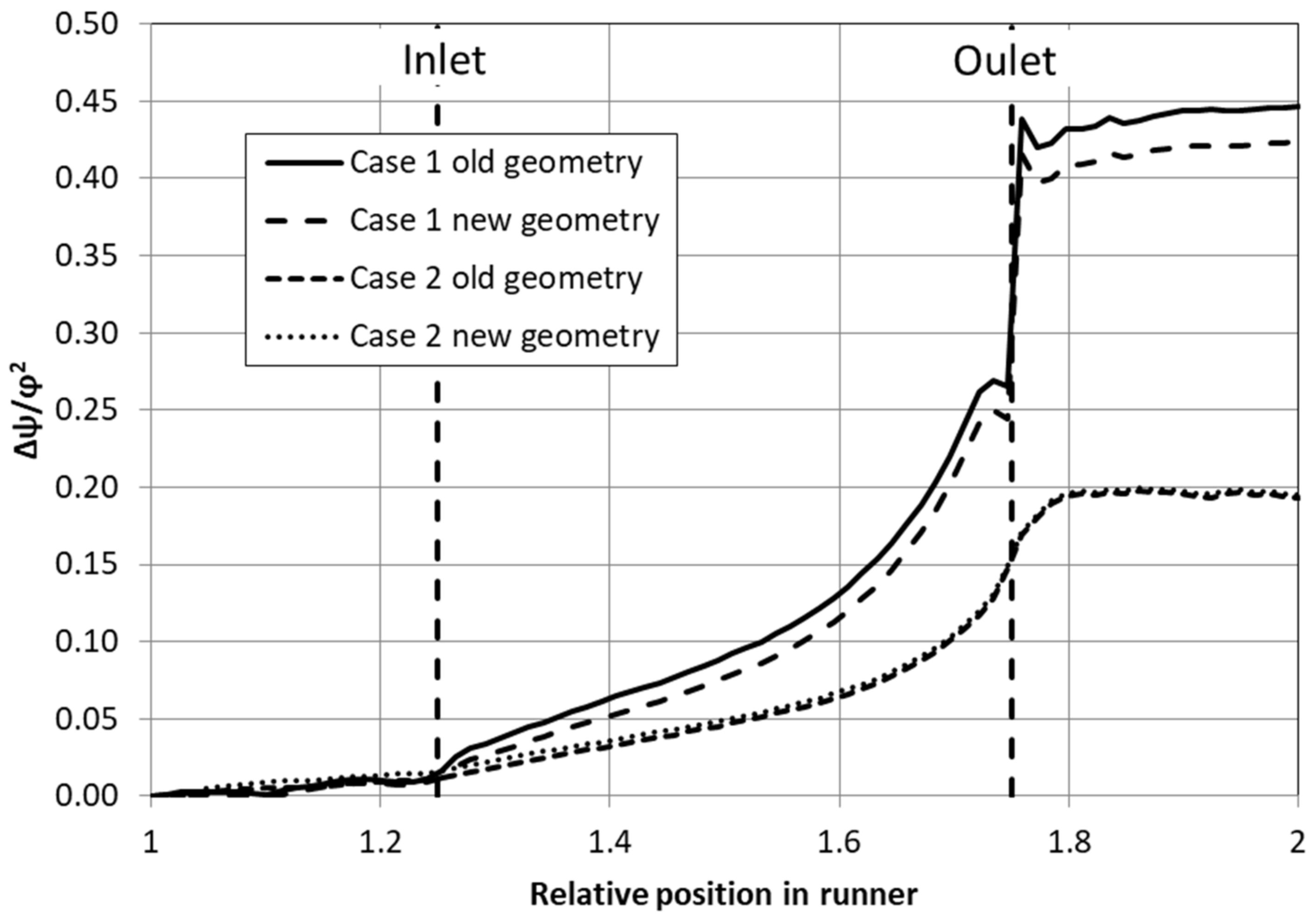
The observation of the efficiency loss coefficient as a function of the relative position in the runner, Figure 19, confirms the greater efficiency losses at the runner inlet in the old geometry of case 1. In comparison, case 2 shows no variation in runner efficiency losses between the two geometries.
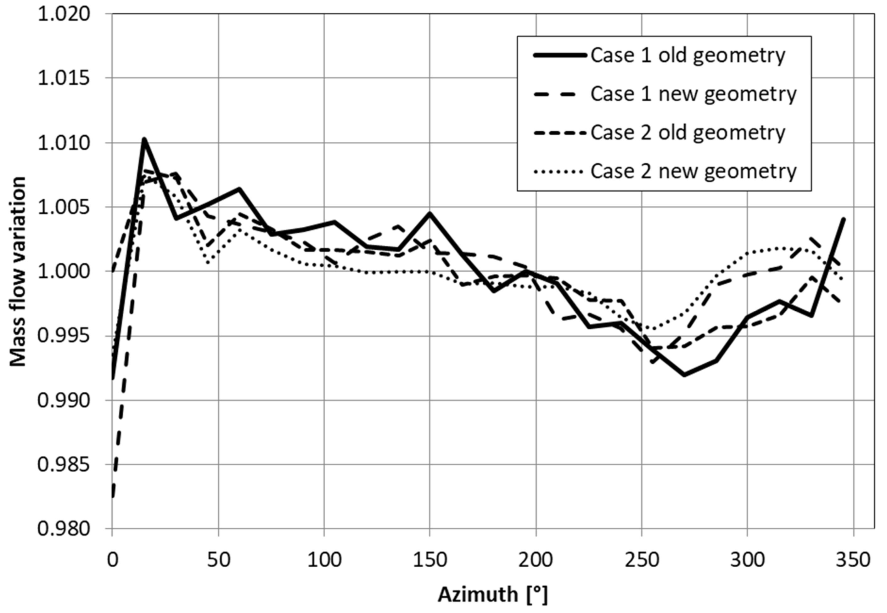
As a comparison of the mass of flow distribution at the GV outlet, Figure 20, shows the absence of differences due to recirculation zones between the old and new geometries. According to this figure, the mass flow distribution is very similar for the two geometries in each case study. The mass flow distribution at the GV outlet is rather a function of the spiral case geometry than of the SV. Thus, since the mass flow distribution is similar in both geometries of the two cases, it does not influence the efficiency losses in the runner. The runner energy head is considered as the main head loss source in the hydraulic turbine and as a factor that has a major effect on the flow uniformity and distribution at the GV outlet.

3.4. Draft Tube

Figure 21 and Figure 22 show the velocity flow obtained with the full turbine simulations at different planes in a draft tube. Some differences are observed between the old and new geometries of the two cases, such as the recirculation zones, characterized by zero flow velocity at the outlet of the draft tube. It is observed that the flow at the beginning of the sluice is quite similar in both geometries, and then small differences appear in the development of recirculation zones. However, the overall topology of the flow is very similar for the draft tube of both the old and new geometries. Indeed, the total area blocked by the recirculation zones at the exit of the draft tube appears to be substantially the same in both geometries, which is why the low-efficiency loss coefficient reduction is evaluated in the new geometry according to the IEC method.
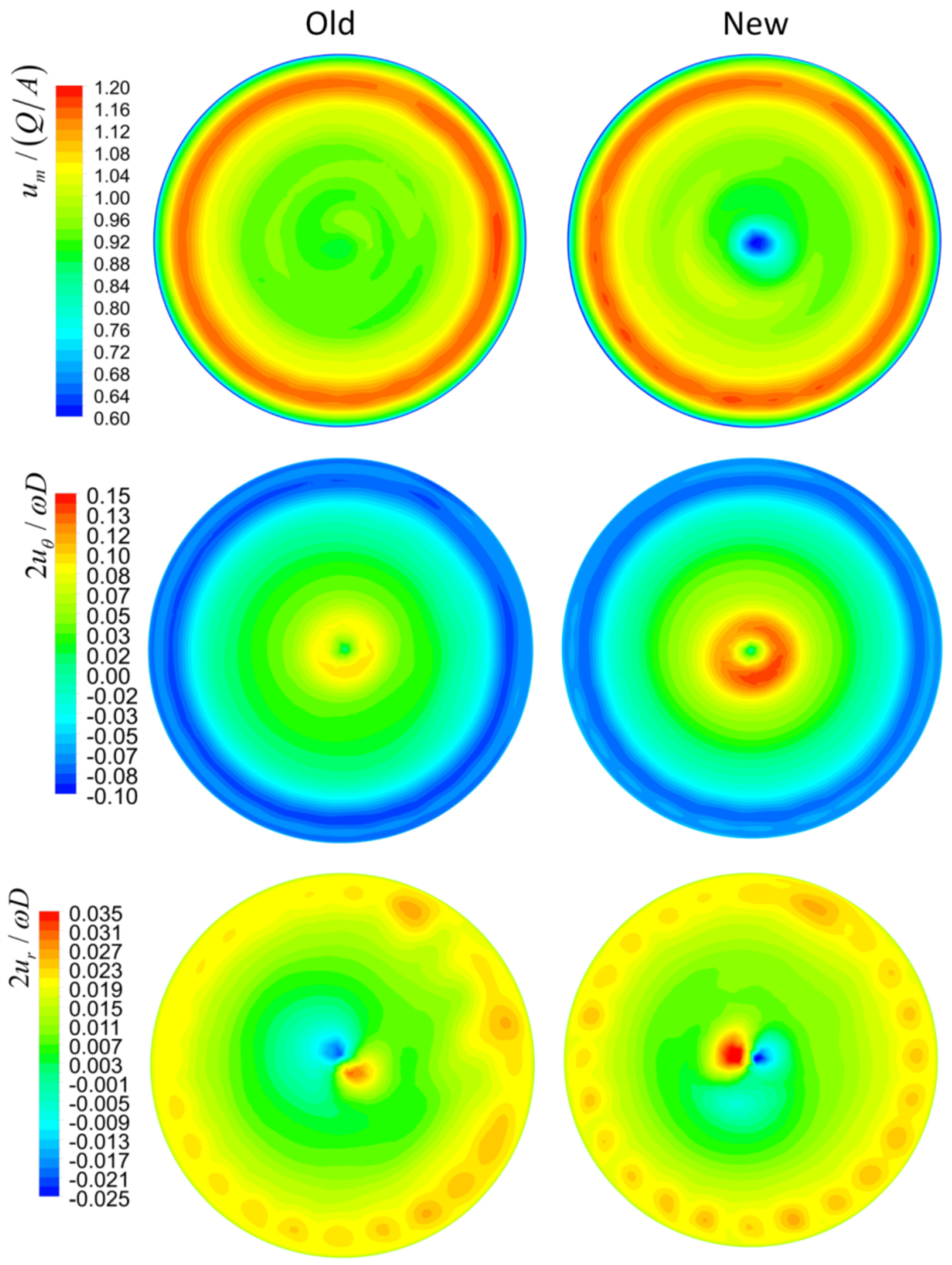
Comparison of the flow at the runner outlet between the old and new geometries of case 1 gives some clues about the slight difference observed in the flow in the draft tube, as exposed in Figure 23, with circumferential, radial, and axial velocities. There are larger differences between the two geometries in the axial and circumferential velocities, due to the mass flow variation imposed at the turbine inlet. In fact, the simulation uses the operating point determined in a test model for each geometry. This implies that there is more circumferential velocity at the runner output in the new geometry, made visible by a larger recirculation zone at the center of the draft tube.
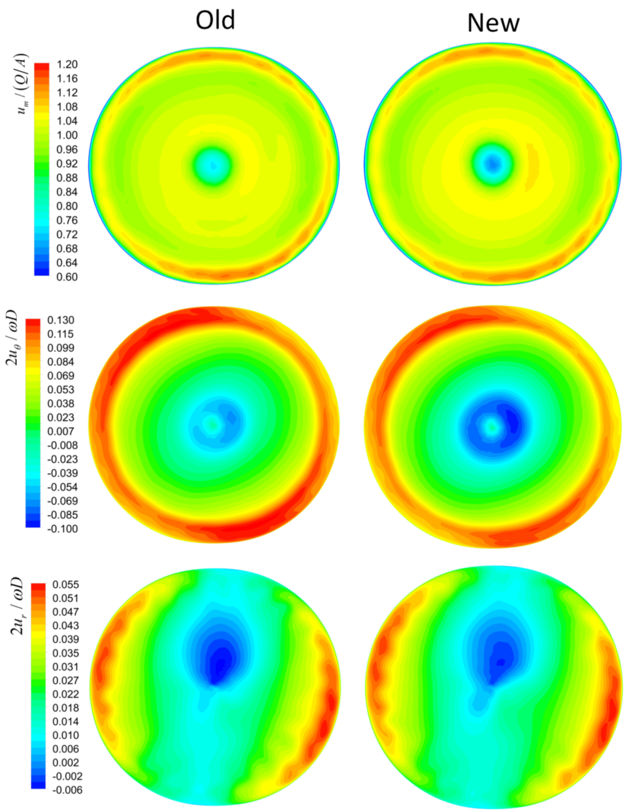
Figure 24 shows that SV modifications bring no significant changes in the velocity fields at the case 2 runner outlet. Note that the significant imbalance of the radial velocity, and to a lesser extent, the axial velocity, is the consequence of the oblong shape of the draft tube cone. In fact, the radial velocity at the wall is mainly led by the divergence angle of the draft tube cone [23]. Due to its particular shape, the divergence angle varies along the perimeter of the tube cone and increases the radial velocity at each side of the oblong. The effect on the axial velocity is similar; where the divergence angle is larger, the more it decelerates the flow.
In both cases, the full turbine simulations do not capture the effect of eliminating the recirculation zones in the tandem cascade at the runner outlet. The change of the mean flow comes from the flow rate imposed at the turbine inlet, as measured in the model tests for the same GVs’ opening. The mean flow at the runner outlet is mainly a function of the flow rate, the runner blade shape, and the rotational speed, according to the velocity triangle [38]. As expected, the numerical simulation shows lower circumferential velocity for the new geometry’s runner outlet, as the flow rate is higher.

4. Conclusions

The full turbine simulation methodology developed is used to model the flow in all of the components of two rehabilitated hydraulic turbines to evaluate their ability to accurately quantify the efficiency increase caused by the SV modification and its effect throughout the turbine in comparison to model tests. The application of this methodology evaluated up to 65% of the model tests’ efficiency increases in case 1 and 40% in case 2. Comparing component-to-component in case 1, the simulation found 57% of the total model tests’ efficiency increases in the SV, 34% in the GV, 11% in the runner, and an insignificant variation in the draft tube. In case 2, 72% of efficiency loss was computed to be in the SV, 39% in the GV, and an insignificant variation in the runner and the draft tube.
In both cases, the elimination of the recirculation zones by the SV modification was determined to be the main cause of the significant efficiency increase in that component. The efficiency increase in the GVs of the new geometry comes from the elimination of the wake due to the recirculation zones at the SV. For both cases, the effect of the SV’s modification is very similar, except for the variation of angular momentum at the GV’s outlet in case 1, where this angular momentum variation between the old and new geometries leads to the efficiency increase in the runner. In the second case, the absence of modification to the average flow at the runner inlet results in the absence of efficiency loss variation in this component. The local disturbances in the flow due to the recirculation zones at the exit of the GVs are reduced by the runner. The absence of efficiency loss variation in the draft tube is explained by the small difference in the flow at the runner outlet.
The methodology of the full turbine simulation developed with URANS equations and the k-ω SST turbulence model appears to reach its limits to accurately assess the overall efficiency losses in the hydraulic turbines studied. The mesh-independence study in each component of the turbine shows the low probability of obtaining a significant efficiency loss change with finer meshes. Finally, it is proposed that further works could use a more complex flow modeling approach to observe if the wake of the boundary layer separation of the SVs and its turbulent structures can influence the flow and efficiency loss in the runner and the draft tube.

Author Contributions

Conceptualization, M.S.; methodology, P.M.R.; software, P.M.R.; validation, P.M.R., A.S. and M.S.; formal analysis, P.M.R. abs A.S.; investigation, P.M.R.; resources, A.S. and M.S.; data curation, P.M.R.; writing—original draft preparation, P.M.R.; writing—review and editing, A.S. and P.M.R.; visualization, P.M.R.; supervision, A.S. and M.S.; project administration, A.S. and M.S.; funding acquisition, A.S. and M.S. All authors have read and agreed to the published version of the manuscript.

Funding

An Industrial Innovation Scholarship provided by the Natural Sciences and Engineering Research Council of Canada (NSERC) and Research Fund of Quebec Nature and Technology (FRQNT) has allowed the realization of this work through its financial support.

Institutional Review Board Statement

Not applicable.

Informed Consent Statement

Not applicable.

Acknowledgments

The permission to use the geometries as well technical and financial support is granted by Alstom Energy & Transport Canada Inc. The simulations were performed on the supercomputers of Compute Canada.

Conflicts of Interest

The authors declare no conflict of interest.

Nomenclature

Notation
Aarea (m2)
cgrid refinement factor
eaapproximate relative error
eextextrapolated relative error
Eenergy head (m)
ggravitational acceleration (ms−2)
GCIfinefine-grid convergence index
Hirunner internal head (m)
Hnturbine hydraulic head (m)
hrepresentative cell size (m)
Nsqhydraulic turbine specific speed (s−1)
m ˙ mass flow (kgs−1)
Ppressure (kgm−1s−2)
pGCI method apparent order
Qdischarge (m3s−1)
rradius (m)
Ttorque (Nm)
tunit of time (s)
uvelocity (ms−1)
umflow velocity (ms−1)
uθcircumferential velocity (ms−1)
urradial velocity (ms−1)
xlength (m)
Y+dimensionless distance
zelevation (m)
γguide vanes opening (°)
εcritical value difference
ηefficiency
φdischarge coefficient
ϕcritical value
ϕextextrapolated value
ψenergy coefficient
Ωrotational speed (s−1)

References

  1. Canadian Hydropower Association. Hydropower in Canada: Past, Present and Future. Available online: http://www.renewableenergyworld.com/rea/news/article/2009/10/hydropowerin-canada-past-present-and-future (accessed on 1 July 2021).
  2. International Energy Agency. Key World Energy Statistics; International Energy Agency: Paris, France, 2008. [Google Scholar]
  3. Eberle, P.; Couston, M.; Sabourin, M. The refurbishment of low head Francis turbines. Int. J. Hydropower Dams 2003, 10, 45–48. [Google Scholar]
  4. Michel, B.; Vuillerod, G.; Francois, M.; Kunz, T. Efficient rehabilitation of hydro generating units. Int. J. Hydropower Dams 2007, 14, 140–146. [Google Scholar]
  5. Michel, B.; Couston, M.; Sabourin, M.; Francois, M. Hydro Turbines Rehabilitation; IMechE Event Publications, 2004; pp. 3–12. Available online: https://www.encyclopedie-energie.org/wp-content/uploads/2018/09/art083_Michel-Bernard-Couston-Michel-et-al_Hydro-turbines-rehabilitation.pdf (accessed on 1 July 2021).
  6. Morris, D.; Froehlich, D.; Hartmann, O. Guides for hydroplant modernization. In Proceedings of the American Power Conference, Chicago, IL, USA, 18–20 April 1988; Volume 50, pp. 1067–1076. [Google Scholar]
  7. Drtina, P.; Sallaberger, M. Hydraulic turbines—Basic principles and state-of-the-art computational fluid dynamics applications. Proc. Inst. Mech. Eng. Part C J. Mech. Eng. Sci. 1999, 213, 85–102. [Google Scholar] [CrossRef]
  8. Suzuki, T.; Nagafuji, T.; Komiya, H.; Shimada, T.; Kobayashi, T.; Taniguchi, N. Flow behavior around stay vanes and guide vanes of a Francis turbine. ASME J. Fluids Eng. 1996, 118, 110–115. [Google Scholar] [CrossRef]
  9. Vu, T.C.; Shyy, W. Performance Prediction by Viscous Flow Analysis for Francis Turbine Runner. J. Fluids Eng. 1994, 116, 116–120. [Google Scholar] [CrossRef]
  10. Vu, T.C.; Shyy, W. Navier-Stokes Flow Analysis for Hydraulic Turbine Draft Tubes. J. Fluids Eng. 1990, 112, 199–204. [Google Scholar] [CrossRef]
  11. Wu, J.; Shimmei, K.; Tani, K.; Niikura, K.; Sato, J. CFD-Based Design Optimization for Hydro Turbines. J. Fluids Eng. 2007, 129, 159. [Google Scholar] [CrossRef]
  12. Keck, H.; Drtina, P.; Sick, M. Numerical Hill Chart Prediction by Means of CFD Stage Simulation for a Complete Francis Turbine. In Hydraulic Machinery and Cavitation; Springer Science and Business Media LLC: Berlin, Germany, 1996; pp. 170–179. [Google Scholar]
  13. Dörlfer, P. Observer-based control of a low-head Pelton plant equipped with a long penstock. In Proceedings of the 2nd Conference on Modeliling, Testing & Monitoring for Hydro Poweplants, Lausanne, Switzerland, 8–11 July 1996. [Google Scholar]
  14. Ruprecht, A. Unsteady flow simulation in hydraulic machinery. Task Q. 2002, 6, 187–208. [Google Scholar]
  15. Kurosawa, S.; Lim, S.M.; Enomoto, Y. Virtual model test for a Francis turbine. In IOP Conference Series: Earth and Environmental Science; IOP Publishing: Philadelphia, PA, USA, 2010; Volume 12. [Google Scholar]
  16. Lain, S.; Garcia, M.; Quintero, B.; Orrego, S. CFD Numerical simulations of Francis turbines Simulación numérica (CFD) de turbinas Francis. Rev. Fac. Ing. Univ. Antioq. 2010, 51, 24–33. [Google Scholar]
  17. Magnoli, M.; Schilling, R. Increase of the annual energy output in hydraulic powerplants through active flow control. Renew. Energy Power Qual. J. 2011, 1148–1153. [Google Scholar] [CrossRef]
  18. Trivedi, C.; Cervantes, M.J.; Gandhi, B.K.; Dahlhaug, O.G. Experimental and Numerical Studies for a High Head Francis Turbine at Several Operating Points. J. Fluids Eng. 2013, 135, 111102. [Google Scholar] [CrossRef]
  19. Wu, Y.; Liu, S.; Wu, X.; Dou, H.; Zhang, L.; Tao, X. Turbulent flow computation through a model Francis turbine and its performance prediction. In IOP Conference Series: Earth and Environmental Science; IOP Publishing: Philadelphia, PA, USA, 2010; Volume 12. [Google Scholar]
  20. Yexiang, X.; Zhengwei, W.; Zongguo, Y.; Mingan, L.; Ming, X.; Dingyou, L. Numerical analysis of unsteady flow under high-head operating conditions in Francis turbine. Eng. Comput. 2010, 27, 365–386. [Google Scholar] [CrossRef]
  21. Zobeiri, A.; Kueny, J.L.; Farhat, M.; Avellan, F. Pump-Turbine Rotor-Stator Interactions in Generating Mode: Pressure Fluctuation in Distributor Channel. In Proceedings of the 23rd IAHR Symposium on Hydraulic Machinery and Systems, Yokohama, Japan, 17–21 October 2006. [Google Scholar]
  22. Maruzewski, P.; Hayashi, H.; Münch, C.; Yamaishi, K.; Hashii, T.; Mombelli, H.P.; Sugow, Y.; Avellan, F. Turbulence modeling for Francis turbine water passages simulation. In IOP Conference Series: Earth and Environmental Science; IOP Publishing: Philadelphia, PA, USA, 2010; Volume 12. [Google Scholar]
  23. Mauri, S.; Kueny, J.-L.; Avellan, F. Werle´-Legendre Separation in a Hydraulic Machine Draft Tube. In Proceedings of the ASME 2002 Joint U.S.-European Fluids Engineering Division Conference, Montreal, QC, Canada, 14–18 July 2002; Volume 1, Fora, Parts A and B. pp. 885–891. [Google Scholar] [CrossRef]
  24. Tridon, S.; Barre, S.; Ciocan, G.; Ségoufin, C.; Leroy, P. Discharge Imbalance Mitigation in Francis Turbine Draft-Tube Bays. J. Fluids Eng. 2012, 134, 041102. [Google Scholar] [CrossRef]
  25. Beaubien, C.A. Simulations Numériques de L’écoulement Turbulent dans un Aspirateur de Turbine Hydraulique; Université Laval: Québec, QC, Canada, 2013. [Google Scholar]
  26. ANSYS, Inc. Release 13.0, ANSYS CFX-Solver Theory Guide; Southpointe: Canonsburg, PA, USA, 2010. [Google Scholar]
  27. Gagnon, J.M.; Deschênes, C. Numerical Simulation with flow feature extraction of a propeller turbine unsteady rotor-stator interaction. In WIT Transactions on Modelling and Simulation; WIT Press: Southampton, England, 2007; Volume 46. [Google Scholar] [CrossRef] [Green Version]
  28. Nennemann, B.; Vu, T.C.; Farhat, M. CFD prediction of Unsteady Wicket Gate-Runner Interaction in Francis Turbines: A New Standard Hydraulic Design Procedure. In Proceedings of the HYDRO 2005 International Conference and Exhibition, Villach, Austria, 17–20 October 2005. [Google Scholar]
  29. Menter, F.; Kuntz, M.; Langtry, R. Ten years of industrial experience with the SST turbulence model. Turbul. Heat Mass Transf. 2003, 4, 625–632. [Google Scholar]
  30. Ciocan, G.D.; Iliescu, M.S.; Vu, T.C.; Nennemann, B.; Avellan, F. Experimental Study and Numerical Simulation of the FLINDT Draft Tube Rotating Vortex. J. Fluids Eng. 2006, 129, 146–158. [Google Scholar] [CrossRef]
  31. Munson, B.R.; Okiishi, T.H.; Huesbsch, W.W.; Rothmayer, A.P. Fundamentals of Fluid Mechanics; John Wile & Sons: Hoboken, NJ, USA, 2013. [Google Scholar]
  32. International Electrotechnical Commission. Determination of the Prototype Performance from Model Acceptance Tests of Hydraulic Machines with Consideration of Scale Effects; IEC TC4, 4, 1987–1981; International Electrotechnical Commission: Geneva, Switzerland, 1991. [Google Scholar]
  33. Pointwise. Pointwise V17. 2013. Available online: http://www.pointwise.com/ (accessed on 1 July 2021).
  34. Rousseau, P.M.; Sabourin, M. Comparison between structured hexahedral and hybrid tetrahedral meshes generated by commercial software for CFD hydraulic turbine analysis. In Proceedings of the 21st Annual Conference of the CFD Society of Canada, Sherbrooke, QC, Canada, 6–9 May 2013. [Google Scholar]
  35. Celik, B.; Ghia, U.; Roache, P.J. Procedure for estimation and reporting of uncertainty due to discretization in CFD applications. ASME J. Fluids Eng. 2008, 130, 078001. [Google Scholar]
  36. International Electrotechnical Commission. Hydraulic Turbines, Storage Pumps and Pump-Turbines-Model Acceptance Tests; International Electrotechnical Commission: Geneva, Switzerland, 1999. [Google Scholar]
  37. Kurokawa, J.; Nagahara, H. Flow Characteristics in Spiral Casings of Water Turbines. In Proceedings of the 13th International Association for Hydraulic Research Symposium on Hydraulic Machinery and Cavitation, Montreal, QC, Canada, 1 June 1986. [Google Scholar]
  38. Logan, E., Jr. Handbook of Turbomachinery; CRC Press: New York, NY, USA, 2003. [Google Scholar]
Figure 1. Modifications to the SV of case 1 (left) and 2 (right).
Water 13 01883 g001
Figure 2. Computational domain of full turbine simulation.
Water 13 01883 g002
Figure 3. Example of full turbine simulation domain geometry.
Water 13 01883 g003
Figure 4. Surfaces and pressure tap locations to evaluate turbine head and components efficiency losses.
Water 13 01883 g004
Figure 5. Transition between prismatic and tetrahedral volume cells.
Water 13 01883 g005
Figure 6. Cut view in volume runner mesh.
Water 13 01883 g006
Figure 7. Draft tube fine mesh upstream pier nose.
Water 13 01883 g007
Figure 8. Hydraulic turbine efficiency of case 1 and 2 with and without SV modifications. Efficiency is relative to the maximal efficiency of the new geometry for each case.
Water 13 01883 g008
Figure 9. Efficiency loss coefficient in the tandem cascade in cases 1 and 2. Flow direction is from the right to the left in the figure. SV and GV position are marked with the vertical dashed lines.
Water 13 01883 g009
Figure 10. Velocity at the tandem cascade horizontal plane in case 1 hydraulic turbine functions of the inlet area of the spiral case and the turbine discharge.
Water 13 01883 g010
Figure 11. Velocity at the tandem cascade horizontal plane in case 2 hydraulic turbine functions of the inlet area of the spiral case and the turbine discharge.
Water 13 01883 g011
Figure 12. Flow velocity at the tandem cascade horizontal plane in case 1 hydraulic turbine functions of the inlet area of the spiral case and the turbine discharge.
Water 13 01883 g012
Figure 13. Flow velocity at the tandem cascade horizontal plane in case 2 hydraulic turbine functions of the inlet area of the spiral case and the turbine discharge.
Water 13 01883 g013
Figure 14. Flow velocity at the tandem cascade horizontal plane functions of the inlet area of the spiral case and the turbine discharge and um = 0 isosurface in case 1 hydraulic turbine.
Water 13 01883 g014
Figure 15. Flow velocity at the tandem cascade horizontal plane functions of the inlet area of the spiral case and the turbine discharge and um = 0 isosurface in case 2 hydraulic turbine.
Water 13 01883 g015
Figure 16. Flow orientation at SV leading edge of the two studied hydraulic turbines.
Water 13 01883 g016
Figure 17. Angular momentum in function of the tandem cascade radius.
Water 13 01883 g017
Figure 18. Streamlines at a runner blade of case 1 old and new geometries.
Water 13 01883 g018
Figure 19. Efficiency loss coefficient as function of relative position in the runner of the case 1 and 2.
Water 13 01883 g019
Figure 20. Azimuthal mass flow variation at GV outlet of case 1 and 2 hydraulic turbines.
Water 13 01883 g020
Figure 21. Flow velocity in the draft tube of old and new geometries of case 1 functions of the inlet area of the draft tube and the turbine discharge.
Water 13 01883 g021
Figure 22. Flow velocity in the draft tube of old and new geometries of case 2 functions of the inlet area of the draft tube and the turbine discharge.
Water 13 01883 g022
Figure 23. Axial, circumferential and radial flows at runner outlet of case 1 hydraulic turbine. Axial velocity is function of the inlet area of the draft tube and the turbine discharge.
Water 13 01883 g023
Figure 24. Axial, circumferential and radial flows at runner outlet of case 2 hydraulic turbine. Axial velocity is function of the inlet area of the draft tube and the turbine discharge.
Water 13 01883 g024
Table 1. Operating points of hydraulic turbines studied.
TitleCase 1Case 2
GeometryOldNewOldNew
γ ° 25252424
φ / φ o p t 0.9981.0021.0021.001
Table 2. Nodes (106) in meshes used for case 1 and 2 spiral case simulations.
TitleCase 1Case 2
GeometryOldNewOldNew
Coarse24.615.19.710.8
Medium28.820.516.220.9
Fine68.422.925.727.9
Table 3. Nodes (106) in meshes used for runner and draft tube simulations.
SimulationRunnerDraft Tube
Coarse0.462.67
Medium0.724.77
Fine1.126.59
Table 4. Spatial discretization error and numerical uncertainties in spiral case and tandem cascade.
TitleCase 1Case 2
GeometryOldNewOldNew
c 21 1.361.041.171.10
c 32 1.051.111.191.25
ϕ 1 (m)0.8180.4740.4870.446
ϕ 2 (m)0.7980.4740.4920.435
ϕ 3 (m)0.7830.4710.4910.437
ε 32 0.0198−0.002910.000230.00222
ε 21 0.0244−0.000330.00435−0.0112
e a 21 0.02440.0007020.008920.0252
G C I f i n e 21 0.0009430.0008590.000429-
Table 5. Spatial discretization error and numerical uncertainties in runner and draft tube meshes.
Sub-DomainRunnerDraft Tube
c 31 1.1591.114
c 32 1.1611.213
ϕ 1 (m)12.314.03
ϕ 2 (m)12.833.58
ϕ 3 (m)11.543.13
ε 32 −1.290−0.450
ε 21 0.520−0.450
e a 21 0.0420.112
G C I f i n e 21 0.0360.063
Table 6. Nodes (106) in meshes used for case 1 and 2 full turbine simulations.
Case 1Case 2
Sub DomainOldNewOldNew
Spiral case39.728.224.928.5
Runner2217.8
Draft tube6.75.6
Table 7. Efficiency losses coefficient reduction evaluate by complete turbine simulation. Model tests values are show as reference.
Title Δ ψ / φ 2 O l d Δ ψ / φ 2 N e w Δ ψ / φ 2 O l d Δ ψ / φ 2 N e w C F D Δ ψ / φ 2 O l d Δ ψ / φ 2 N e w C F D   T o t a l   %
Case1212
Spiral case0.001−0.002~0−4
Stay vanes0.1370.0325772
Guide vanes0.0810.0173439
Runner0.025−0.00111−3
Draft tube−0.004−0.002−2−4
Total0.2400.044100100
Model tests0.3670.111--
Table 8. Flow orientation misalignment at the leading edge of the stay vanes of case 1 and 2.
GeometryOldNew
Case 114.2°6.1°
Case 223.8°4.2°
Publisher’s Note: MDPI stays neutral with regard to jurisdictional claims in published maps and institutional affiliations.

