Article

A Model Tree Generator (MTG) Framework for Simulating Hydrologic Systems: Application to Reservoir Routing

1
Center for Hydrometeorology and Remote Sensing (CHRS), Department of Civil and Environmental Engineering, The Henry Samueli School of Engineering, University of California, Irvine, CA 92697, USA
2
School of Civil Engineering and Environmental Science, University of Oklahoma, Norman, OK 73019, USA
3
Coastal and Hydraulics Laboratory, U.S. Army Engineer Research and Development Center, Vicksburg, MS 39180, USA
4
Earth System Science Interdisciplinary Center, University of Maryland, College Park, MD 20740, USA
5
Department of Earth System Science, University of California Irvine, 3200 Croul Hall, Irvine, CA 92697, USA
*
Author to whom correspondence should be addressed.
Water 2020, 12(9), 2373; https://doi.org/10.3390/w12092373
Submission received: 30 June 2020 / Revised: 19 August 2020 / Accepted: 21 August 2020 / Published: 24 August 2020
(This article belongs to the Special Issue Spatial Modelling in Water Resources Management)

Abstract

:
Data-driven algorithms have been widely used as effective tools to mimic hydrologic systems. Unlike black-box models, decision tree algorithms offer transparent representations of systems and reveal useful information about the underlying process. A popular class of decision tree models is model tree (MT), which is designed for predicting continuous variables. Most MT algorithms employ an exhaustive search mechanism and a pre-defined splitting criterion to generate a piecewise linear model. However, this approach is computationally intensive, and the selection of the splitting criterion can significantly affect the performance of the generated model. These drawbacks can limit the application of MTs to large datasets. To overcome these shortcomings, a new flexible Model Tree Generator (MTG) framework is introduced here. MTG is equipped with several modules to provide a flexible, efficient, and effective tool for generating MTs. The application of the algorithm is demonstrated through simulation of controlled discharge from several reservoirs across the Contiguous United States (CONUS).

1. Introduction

Data-driven models are effective tools for simulating nonlinear and complex systems, and have been widely used for regression and classification problems [1,2]. These models rely on statistical and numerical approaches for simulating the underlying system, rather than employing physics-based equations [3,4]. Among data-driven approaches decision tree (DT) algorithms offer transparent representations of systems [5,6], in contrast to black-box models with uninterpretable or hidden logic [7]. The DT algorithms describe and represent a dependent (response) variable by partitioning the independent (explanatory) variables’ space into clusters of data [8,9]. Simplicity and accuracy of DT algorithms make them attractive tools among practitioners in different fields of study [10], including remote sensing [11,12,13], water resources management [14,15,16,17,18] and hydrology [19,20].
Although, classic DT algorithms were originally more concerned with classification and discrete spaces [21], applications of the DT models have since been extended to regression problems and continuous spaces through the development of regression trees induction methods [10]. A wide range of algorithms have been proposed for regression tree induction, among which Classification And Regression Tree (CART) [22] has found many applications in water resources management studies [15]. A popular class of these regression tree algorithms is model tree (MT) [23], which employs piecewise linear models to predict numerical values [24,25]. Among MT algorithms, M5 and M5′ [21,25] have been used in several studies in the fields of water resources management and hydrology [26,27,28,29,30,31,32,33].
Although MT algorithms have been shown to be effective tools for high dimensional numerical datasets [34], their induction approaches can be computationally intensive for large datasets with multiple attributes [35]. These algorithms evaluate almost every single instance in the data to form the structure of the model. Moreover, the choice of the induction criterion can affect the accuracy of the resulted model [36], and can further increase the computational burden of these algorithms. Hence, the exhaustive approaches can hinder the application of these induction methods to large datasets. Here, we introduce a Model Tree Generator (MTG) framework to tackle these shortcomings. The MTG framework is designed to be flexible and efficient in employing different induction approaches, while providing effective models for representing the underlying system. The MTG framework provides various settings to enhance the induction speed of the MT algorithms, while maintaining the accuracy of the resulted models.
To evaluate the MTG framework, we first test the proposed method on multiple benchmark machine learning datasets to better understand the effect of the speed enhancement modules and settings on the performance and accuracy of the resulted models. These machine learning test cases have been employed for evaluating various machine learning algorithms [37]. Due to the importance of reservoirs role in water resources management and hydrology [38], we then employ the algorithm to generate models for simulating controlled discharge from multiple reservoir systems across the Contiguous United States (CONUS). The MTG framework, is compared with CART and M5′ on all these case studies.
The rest of the paper is organized as follows. Section 2 provides a brief background on DT models and outlines the scope of this work. Then it introduces the newly developed MTG framework and explains the underlying algorithm. Details of the case studies and settings are presented in Section 3. Section 4 presents the results for the machine learning and reservoir case studies and discuss the speed enhancement of the MTG framework. Section 5 concludes the paper and elaborates on the performance, limitations, and future works of the MTG framework.

2. Materials and Methods

2.1. Background and Scope

DT algorithms are non-parametric supervised learning approaches which provide interpretable and accurate representation of the underlying system [39]. Binary decision trees are the simplest form of DT models [39] which employ a set of true-false tests, T = T 1 x i , , T t x i , to predict the class or value of a dependent variable, Y = y 1 , , y n , according to a set of independent variables, X = x 1 , , x n [40]. These true-false tests are constructed within a procedure, so-called tree induction, such that the number of required tests ( T ) is minimal for the training data set, X = x i , y i : i = 1 , , n , for the resulted model [40]. The tree induction procedure in binary regression tree algorithms identifies these tests by successive recursive binary splits of data ( X ) on all independent variables x i and cut points ( c ) selected from the training data [41]. This selection is carried out using a predefined measure of impurity or representativeness [42], such as the sum squared residuals [10], which evaluates the difference between the prediction skill of data before (parent), and after (child), partitioning. This splitting mechanism is repeated until the stopping criterion is satisfied. The selected variables and cut points form the true-false tests as inequalities ( x i c and x i > c ) [41] and are evaluated in the order they are constructed within the structure of the inducted model.
The resulted model has a hierarchical if-then tree-structured form and consists of two types of nodes, non-terminal (decision) nodes and terminal (leaf) nodes. The non-terminal nodes navigate the instances through the branches of the tree towards terminal (leaf) nodes by the tests ( T ) constructed during the tree induction procedure. The terminal nodes then simulate the target values using classes, values or functions ( f 1 x i , , f m x i ) derived during the tree induction process. The gateway for input data in the DT model is the top non-terminal node, so-called the root node. Figure 1 shows the structure of a binary DT model (right) inducted for a synthetic dataset with the split lines (cut points) partitioning the independent variables (left). Each partition of data is presented by a terminal node.
After forming the structure of the model, DT induction algorithms employ different approaches to specify the classes, values, or functions in the terminal nodes. Many algorithms, such as CART [22], report the most frequent class or average value of the numerical dependent variable of each partition as the node value. MTs, on the other hand, employ multiple linear regression at terminal nodes [24], which makes them suitable for high dimensional continuous problems [34]. Many MT algorithms follow a binary splitting mechanism. In these algorithms, an exhaustive search approach is employed to select variables and cut points [42]. In most MT algorithms, all values of the independent variables are treated as candidate cut points. Hence, all the variables and their values are evaluated to find the best cut points. This search mechanism is computationally inefficient [35], especially for finding the combinatorial effect of independent variables [10]. Here, we introduce a binary Model Tree Generator (MTG) framework for MT induction to address these shortcomings of the MT induction algorithms. The MTG framework provides an efficient MT induction approach for generating models for numerical domains.

2.2. Model Tree Generator Scheme

The MTG framework follows two main steps to generate binary MTs. First, it follows a top-down binary tree induction mechanism to shape the structure of the trees by identifying the tests ( T ) in non-terminal nodes. Second, multiple linear regressions are fitted to the dependent variables in the terminal nodes. Figure 2 shows the schematic representation of the binary MT induction process in the MTG framework. In this process, parent nodes are recursively partitioned into two child nodes, until no further splitting is possible. Then a multiple linear regression model is fitted to each terminal node. MTG is equipped with different splitting criteria and the partitioning process is carried out according to the selected splitting criterion (SC).
The choice of SC can significantly affect the structure and performance of the resulted model [36]. In general, many regression tree algorithms employ a least square criterion for finding the cut points. For instance, the CART algorithm splits data such that the sum squared residuals with respect to the mean of dependent numerical variable is minimized for all the subsets [12,22]. The sum squared residuals with respect to the mean of dependent variable (SSRM) can be defined as,
SSRM = SSRM = n = 1 N y n y ¯ 2 ,
where y n is the observed dependent variable, y ¯ is the mean of observed dependent variables in the subset (node), and N is the number of instances in the subset region. CART calculates SSRM for all the subsets and selects the split candidate which offers the lowest SSRM for resulted subsets. Similar to the CART algorithm, M5 and M5′ select attributes and cut points by maximizing the expected error reduction [21,25]. The attributes and cut points which maximize the standard deviation reduction (SDR) will be selected for generating the subsets in M5 and M5′. SDR can be defined as,
SDR =   s d Y   m = 1 M Y m Y × s d Y m ,
where s d ( ) is the standard deviation operator, Y is the vector of target values, Y m is the vector of target values in the subset m , M is the number of subsets, which is two in the binary DTs (i.e., M = r i g h t ,   l e f t ) and . determines the size of the vectors. Later, Huang and Townshend [12] proposed a stepwise regression tree approach which clusters data by minimizing the sum of distances between each data point and a fitted line to the subset. In this method, sum squared residuals using multiple linear regression (SSRML) can be derived as,
SSRML   =   n = 1 N y n f θ ,   x n 2 ,
where f . , . is the regressed linear function, and x n and θ signify the vector of attributes and coefficients employed in the linear regression, respectively. Huang and Townshend [12] employed stepwise linear regression (SLR) to remove the effect of multi-collinearity of the attributes.
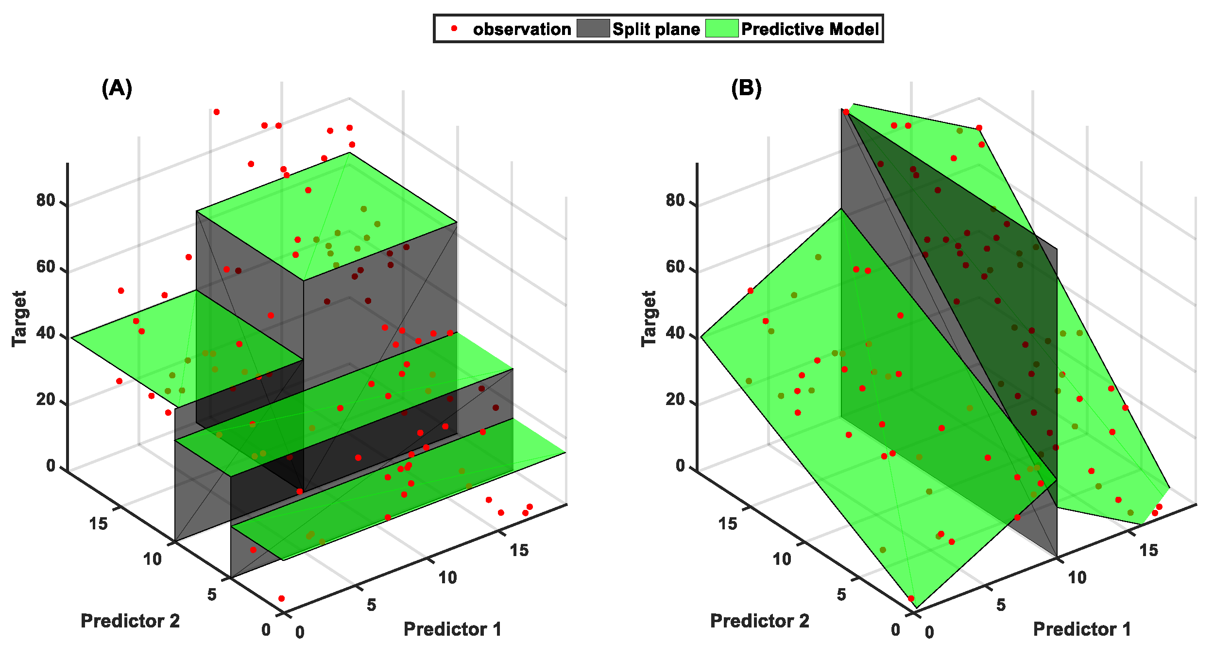
The MTG framework is equipped with these three SC mentioned above; however, it also allows employing other criteria for tree induction, which can be implemented as a function. The MTG framework employs SSRML as the default SC, as MTs employ multiple linear regression in the terminal nodes and SSRML also employs linear regression for splitting. Figure 3 shows an example to demonstrate the difference between employing SSRML and SSRM as SC in the resulted model. In this example, a conceptual dataset with a single dependent variable and two independent variables is represented by the models inducted by MTG framework. The left plot (A) shows the model generated by SSRM setting and constant values in terminal nodes (similar to CART algorithm), and the right plot (B) shows the model generated by SSRML and multiple linear regression in the terminal nodes. In this figure, the regressed and split hyperplanes are shown in green, and gray, respectively. The figure shows the effectiveness of SSRML in combination with multiple linear regression in presenting a continuous numerical dataset. The right plot (B) uses a single split plane and two regression planes to describe data, while the left plot (A) employs three split planes and four constant values for the clusters. This shows that the model generated by SSRML has fewer non-terminal nodes and offers a simple structure in comparison to SSRM. Figure 3 also shows the superiority of linear regression to single constant values for representing subsets of data. It is worth noting that SSRML is the same as the SSRM when the fitted function is constant value. Therefore, SSRML is the general form of SSRM. The presented example in Figure 3 have linear patterns; however, the concept can be extended to non-linear cases, which will be demonstrated in the case studies.
Most MT algorithms employ splitting criteria in an exhaustive search mechanism to form the structure of the tree. However, employing SSRML or similar criterion as SC requires fitting a multivariate linear model to every possible subset of data resulted from each split candidate. This evaluation mechanism is inefficient and computationally intensive. To overcome these shortcomings and enhance the induction process of the MT algorithms, two modules are employed within the MTG framework. First, the algorithm employs a pre-specified number of equidistant quantiles ( ρ ) of attributes as split candidates. In this process, the quantiles are derived empirically for the sorted values of each independent variable. The cumulative probability of each value is empirically calculated using Hazen [43,44] plotting position as,
F x x = r 0.5 N ,
where r is the rank of the sorted values and N is the total number of values. Then equidistant quantiles of data are selected according to these probabilities as the candidate cut points. These selected candidates are employed to split data to subsets. This approach can significantly reduce the number of split candidates while spanning the range of values for each attribute. MTG use 100 equidistant quantiles as the default value which can be modified and customized by the user subject to the problem.
Second, MTG supports local dimension reduction. The local dimension reduction approach allows reducing the number of attributes by considering the correlation and variability of attributes at the subset (node) level. We employ principal component analysis (PCA) for dimension reduction within the MTG framework. PCA is an effective tool for monitoring, restoring, and reducing dimensions of data [45,46]. MTG can employ PCA for dimension reduction of the independent variables in the parent node to reduce the computational burden of regression for deriving SSRML. Since regression is repeated for every subset of the parent node resulted from the split candidates, dimension reduction can significantly reduce the computational burden of the algorithm for large datasets. This also guarantees a well-posed regression problem [47]. MTG selects the principal components (PCs), which describe 99.99% of the variability of independent variables. This step can remove redundancy and noise in data to some extent [48]. However, it can also remove some information from data and increase the error of linear regression [49]. Here, PCA is employed solely for improving the induction speed of MTG for application to large datasets. Interested readers can refer to [47] for further details on PC regression. It is noteworthy that the PC transformation is only used for evaluating the SC to select the best independent variable and split candidate. This process is different from applying PCA to the input data, which is a common practice in data mining. Here, raw data is used to form the true-false tests ( T ) and regressed lines in the non-terminal and terminal nodes to maintain transparency of the final model.
The MTG framework is also equipped with different mechanisms to control the size of the resulted models and avoid over-fitting data. It employs two criteria to stop partitioning dataset and control the number of branches. These stopping criteria reduce the depth of the tree, which is the longest path between the root node and any terminal node in the tree. The depth of the tree resembles the complexity of the inducted model. In most cases, deeper trees have more branches and complexity and may overfit the training data. The first stopping criterion employed within the MTG framework is the minimum leaf size (μ) which determines the minimum number of instances in the terminal node. The minimum leaf size is one of the main controlling parameters in most tree induction algorithms. Another stopping criterion in MTG is the amount of accuracy in terms of RMSE achieved by splitting the parent node. After selecting the best independent variable and cut point for the parent, RMSE values are used to compare the performance of the child nodes with their parent node in terms of prediction accuracy. Partitioning will only occur if child nodes are more accurate than their parent node by a specified amount. MTG uses 5% as the default value for the minimum improvement resulted from splitting the parent node. This means that partitioning will only occur if splitting will improve the accuracy of the node by at least 5%.
After shaping the structure of the trees, MTG fits multivariate lines to each terminal node by least squared residual regression using the original independent variables (not the PC transformed ones). The regressed line is further simplified by employing a backward elimination process. In this process, variables are removed in a stepwise procedure, one at a time and Bayesian Information Criterion (BIC) [50,51] is calculated for the lines fitted to the rest of the variables. The set of variables with the lowest BIC is selected at each step. This process is repeated until removing more variables does not reduce BIC. For convenience, residuals are assumed to be independent and identically distributed with normal distribution [52,53]. Hence, the BIC equation can be stated as,
BIC   =   D ln n + n ln SSR n ,
where D is the dimension of the problem, ln is the natural logarithm operator, and n is the number of instances in the terminal node. BIC penalizes the number of parameters employed in the model [54]. Hence, it simplifies regressed lines in the terminal nodes. This can reveal the importance of independent variables in describing the dependent variables in each subset of data.

3. Case Study

3.1. Machine Learning Test Cases

The MTG framework is tested on multiple datasets from the machine-learning repository of the University of California, Irvine [55]. The selected datasets are different in size and number of attributes. These datasets have been extensively used for evaluating and comparing machine learning algorithms [37]. We employ these datasets to evaluate different components and modules of the MTG framework and recommend the most suitable settings that can be applied to a wide range of datasets. Detailed information on the selected datasets are listed in Table 1.

3.2. Settings of the MTG Framework for Machine Learning Datasets

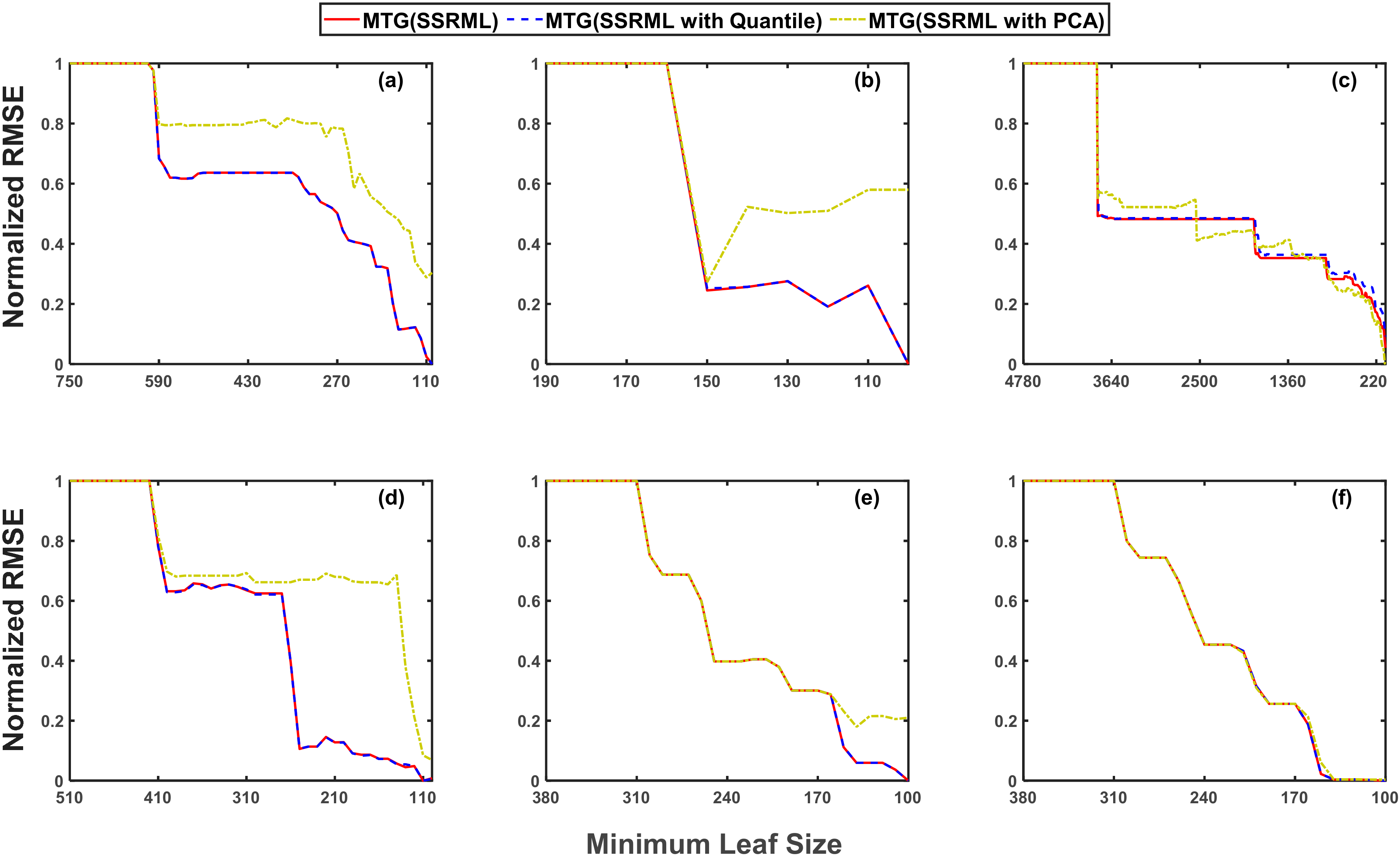
The MTG framework provides two modules to enhance the induction speed of MTs. We apply these modules individually to understand the trade-off between the accuracy of the resulted models and the speed enhancements achieved by each of these components. Since the minimum leaf size value can significantly affect the performance of the resulted model, we carry out our analysis for different leaf size values. We also perform a K-fold Cross-Validation (KCV) to evaluate the resulted models on the validation data. Figure 4 shows the normalized mean RMSE values for KCV with 5 folds for different leaf sizes for validation data. The minimum leaf size values are shown in descending order. Since the minimum leaf size controls the depth of the inducted trees, smaller values of this parameter can be attributed to larger and deeper models. The performance of the resulted models generated by MTG with an exhaustive search method, MTG with quantile sampling and MTG with PCA dimension reduction, are shown in red, blue, and yellow color, respectively. The comparison of the RMSE values shows that the quantile sampling method does not affect the performance of the resulted models. Hence, it can effectively reduce the number of candidates’ cut points without affecting the inducted model. On the other hand, the performance of the models is affected by the PCA dimension reduction method in almost all the cases, when minimum leaf size is getting smaller (the resulted model is deeper). This behavior is due to the variance-based dimension reduction of PCA, which can result in removing information from data. However, the performance of the resulted models is less affected by PCA for large minimum leaf size values (shallow MTs). Therefore, we employ the quantile sampling method as the default search approach, and we apply PCA as an additional option for larger datasets in the rest of the study.
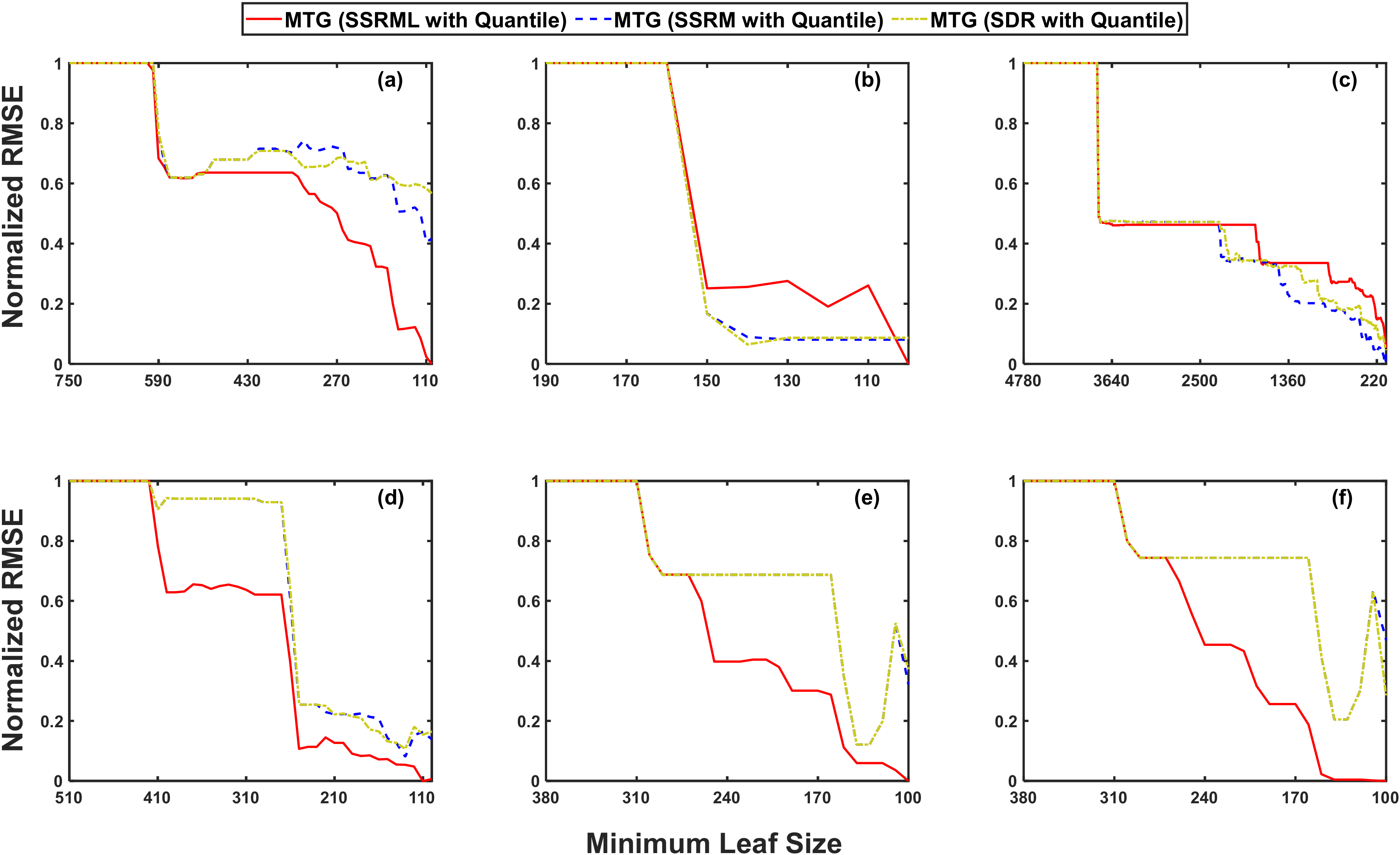
The MTG framework is also equipped with different SC for tree induction. Figure 5 shows the performance of the inducted models generated by MTG using SSRML, SSRM and SDR for different leaf sizes for validation folds. Since the quantile sampling search method was observed to be effective for finding the best point for splitting data, we use this setting for our analysis. In almost all the cases, except case c, the lowest RMSE is achieved by the SSRML criterion. In case; (c), the performance of all the resulted models is very close and is less affected by the selection of SC. This shows that the SSRML criterion has better performance than SSRM and SDR when it is used with regressed lines in the terminal nodes. Hence, for the rest of the study, we employ the SSRML criteria as the default setting of the MTG framework.
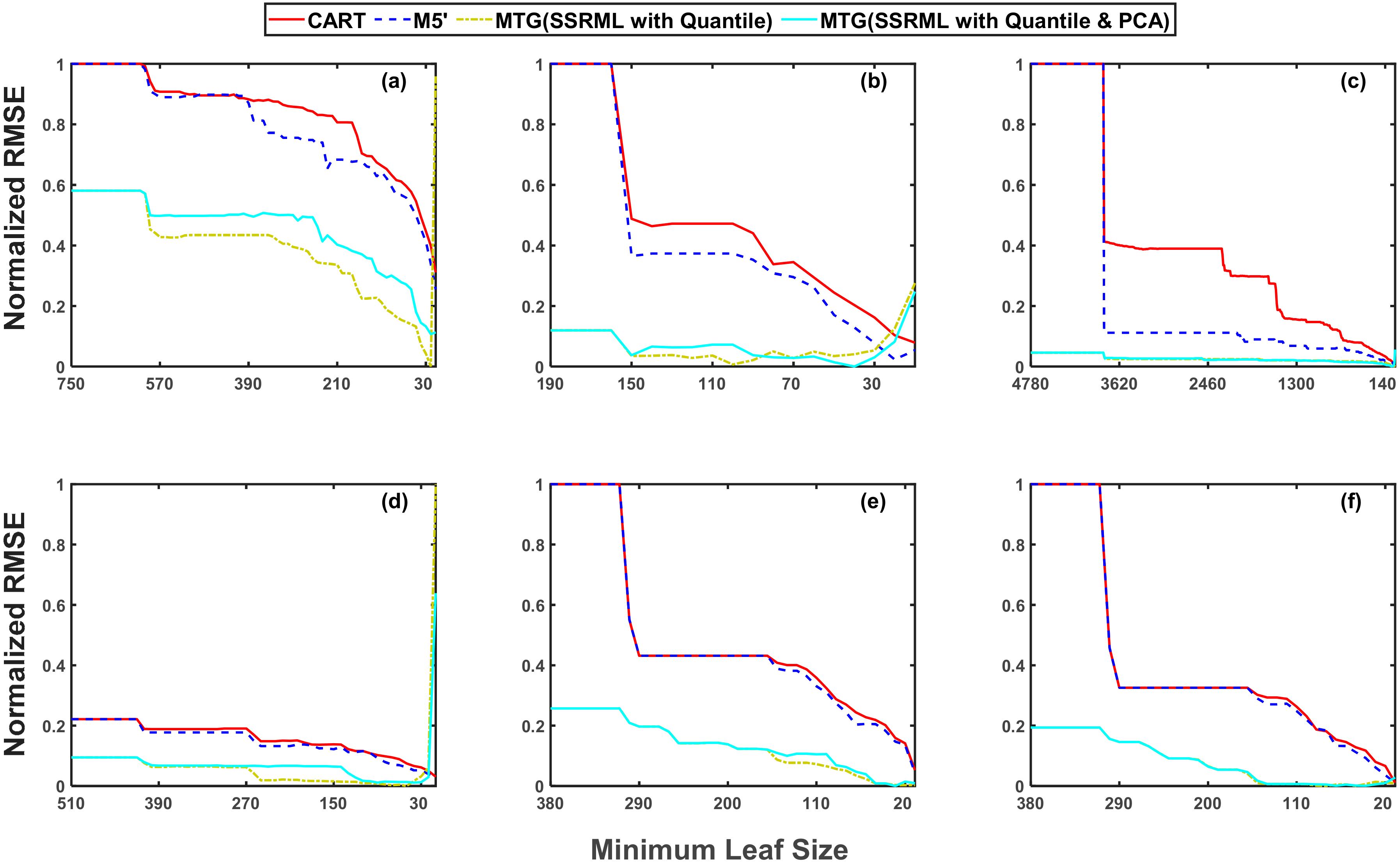
Figure 4 and Figure 5 also highlights the sensitivity of the resulted models to the minimum leaf size values. Hence, careful consideration should be devoted to the selection of these values. We investigate the performance of the models to find the best minimum leaf size value for each of the algorithms for each case study. Since we are comparing CART and M5′ with MTG, we included them in the minimum leaf size analysis to find the minimum leaf size value for those algorithms. Figure 6 shows the normalized RMSE values for CART, M5′, MTG default setting (SSRML with Quantile sampling) and MTG default setting with dimension reduction (SSRML with Quantile sampling and PCA dimension reduction) for different minimum leaf size for validation data. The information from this figure is employed to find the most suitable minimum leaf size value for the algorithms. It is worth noting that the MTG framework error increases for very small minimum leaf size values as the number of samples for regression is very small in these cases. Table 2 lists the minimum leaf size values obtained for each of the algorithms. Since the quantile sampling method has no effect on the accuracy of the resulted models, we use this setting for minimum leaf size analysis. We use these values for the rest of our analysis. The rest of the settings for CART and M5′ and the MTG framework is set to default values. The settings of the MTG framework is listed in Table 3. Hereafter, MTG(SSRML), MTG(SSRML with Quantile), and MTG(SSRML with Quantile and PCA) are referred as MTG(1), MTG(2) and MTG(3), respectively.

3.3. Reservoir Routing Simulation

Reservoirs play an essential role in providing resilience against flood and drought [56] and supply a wide range of services such as, water supply, hydropower electricity, recreation, and ecosystem protection [57,58]. Hence, operators need to address these conflicts among various services, while abiding regulations [59,60]. In practice, the storage-release relationships, known as rule curves, are used for operating reservoir systems [15,61]. Therefore, to simulate these systems, physics-based reservoir models require detailed information about the operation rules and constraints of systems to mimic reservoir operation. The application of physics-based models can be restricted by their complexity due to these existing details [62]. Furthermore, operators may deviate from these rules based on the constraints and conditions of the reservoir, especially in response to extreme weather events [63]. Therefore, physics-based models are typically constrained by pre-defined operating rules, which may not be followed in real-life applications.
On the other hand, recent advancements in the computational efficiency of high-resolution river flow modeling have changed the river flow modeling paradigm from local to high-resolution continental scale [64,65,66,67,68,69]. The implementation of a continental-scale modeling system offers unprecedented insight into river system dynamics [70,71,72]. However, modeling surface water is a real challenge without the inclusion of reservoirs and can result in a non-realistic representation of actual surface water flows [73]. Tavakoly et al. [68] showed that including controlled discharge of the reservoirs in hydrologic models can potentially gain 12–150% accuracy in streamflow simulation of the river basin. Therefore, reservoir routing models play a significant role in the performance of the hydrologic models. Data-driven models can be employed as effective tools to mimic human decision-making in these systems. These models can simulate the effect of reservoir systems within hydrologic models for river routing to enhance the accuracy of streamflow simulation. These algorithms generate models for reservoir routing using the available historical data, without any information about operation rules and constraints of the system [15]. Here, we examine the potential application of the MTG framework for generating reservoir routing models. The MTG framework along with CART and M5′ are employed to simulate controlled daily discharge from eight reservoirs to evaluate the performance of these algorithms on generating models for continuous systems. Similar to the machine learning case studies, we first find the minimum leaf size value for each algorithm. We use the minimum leaf size to generate models for each case study.
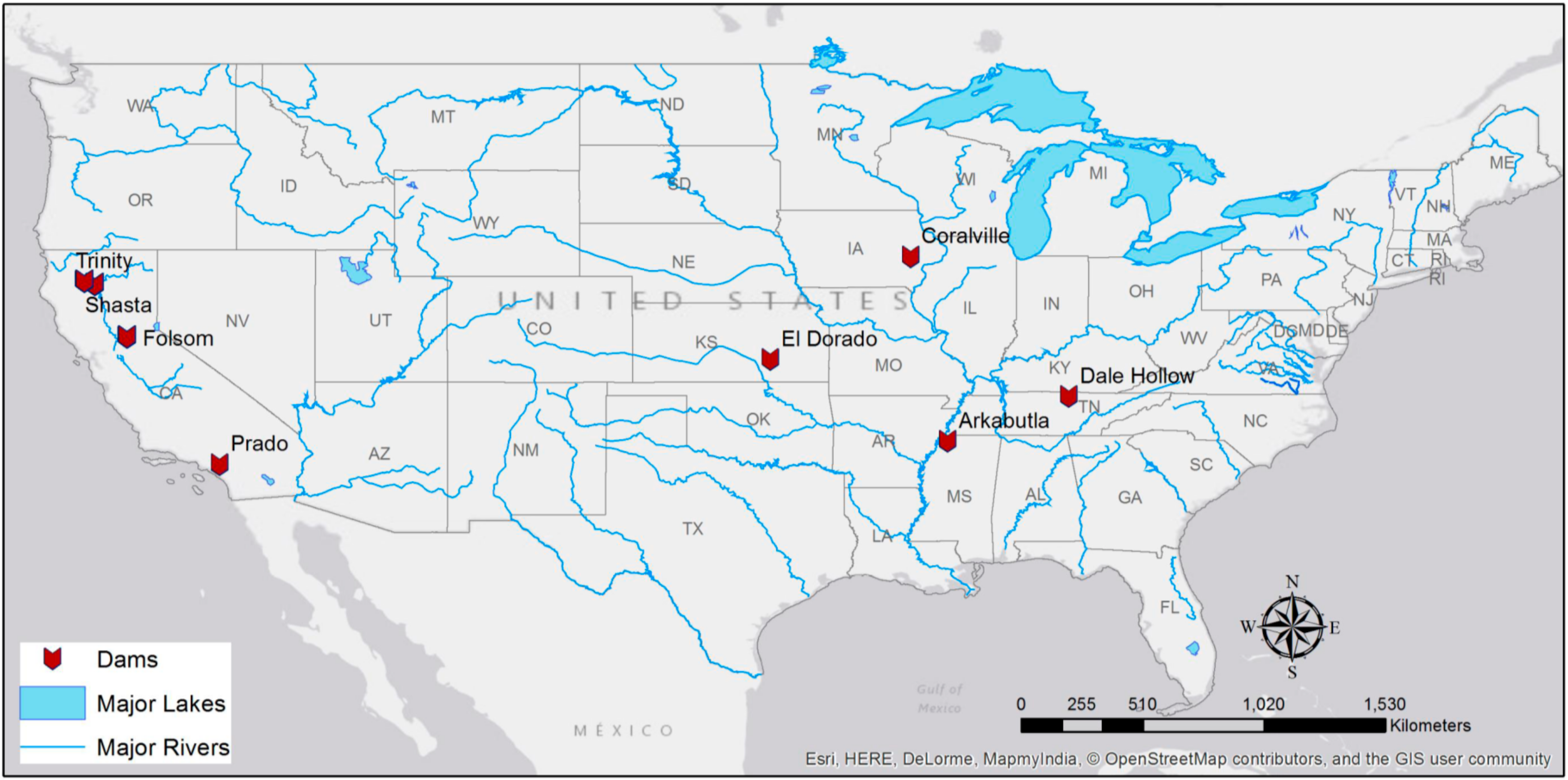
For this study, we selected eight reservoirs with a different range of services. Figure 7 shows the location of these reservoirs across the CONUS. The selected reservoirs provide various services including flood control, water supply, recreation, and hydropower. Four of these reservoirs provide hydropower among which three of them are in California. For most selected reservoirs, the study period covers more than 10 years. However, nine years of data is used for Coralville dam due to the availability of data. Table 4 lists details of the selected reservoirs along with the period of data and hydrologic variables used for these case studies.
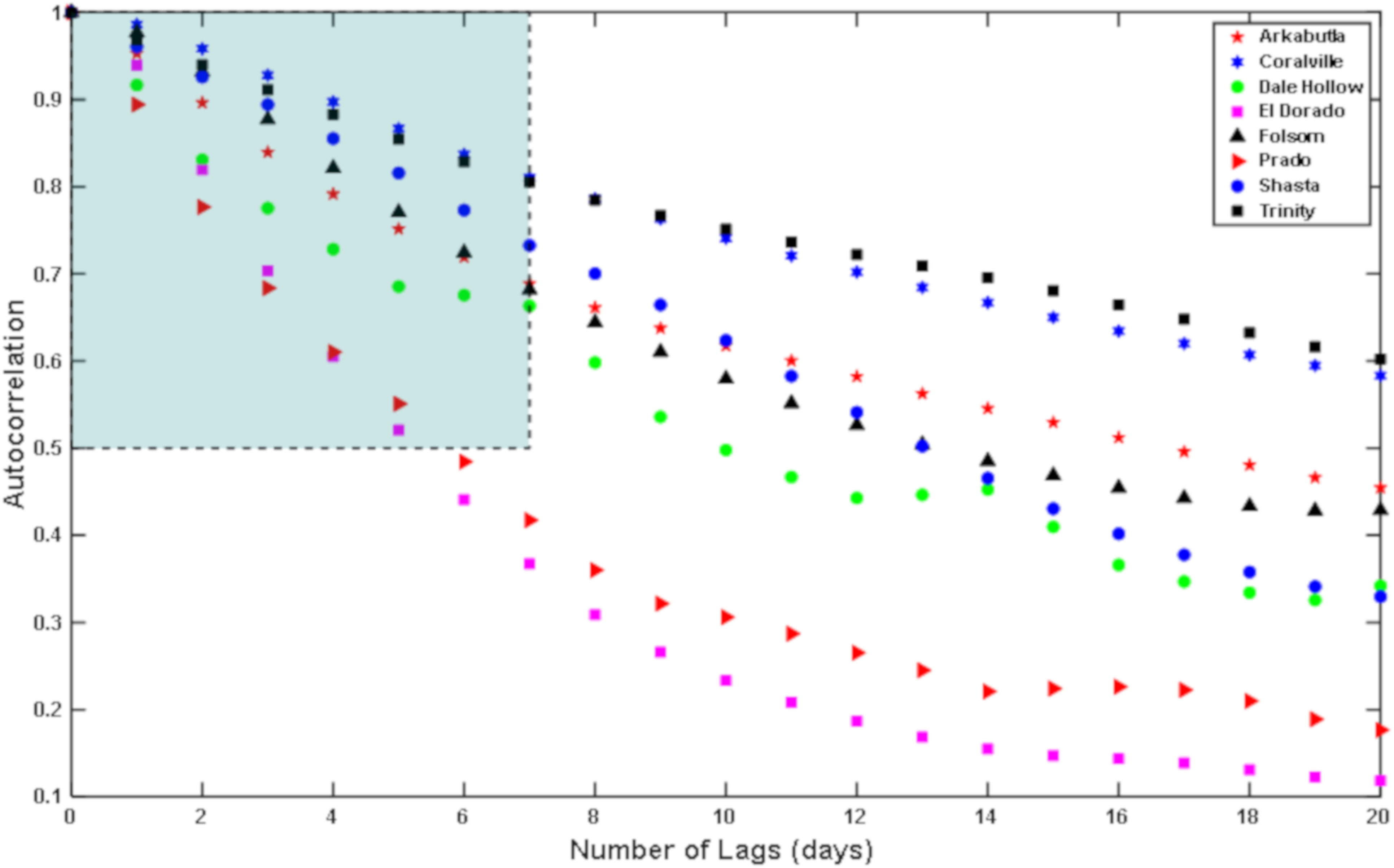
Since MTG, CART, and M5′ algorithms are evaluated and compared for reservoir routing, we only employ storage and inflow data (as input) to simulate discharge (output of the model) from reservoirs in all the case studies. This information can be obtained within most physics-based hydrologic models. In addition to these information, lagged discharge data is also suggested as an indicator for reservoir releases [74]. However, the lagged discharge data is not considered here, due to the high autocorrelation [75] of this data. Figure 8 shows autocorrelation for the discharge data for the selected reservoir cases for different lagged time. For almost all the selected reservoirs, autocorrelation remains above 0.5 after seven lags (days). Due to the high autocorrelation, MT algorithms tend to use lagged data for regression in the terminal nodes. However, employing lagged discharge can propagate error and increase error in long term simulations. Hence, storage and inflow information are the only input information used for these algorithms. It is possible to provide additional information to the tree induction algorithms by providing lagged storage and inflow data. However, lagged discharge can be calculated from the lagged storage and inflow data and can result in error propagation. Yet, lagged data can provide additional information about the previous state of the reservoir and seasonality. In order to provide this information, average storage, and inflow data in last 7, 14, and 30 days are used instead of lagged data in addition to current inflow and storage condition for all the case studies. Hence, eight attributes are employed as input to the algorithms upon data availability. Due to the availability of data for Coralville reservoir, only inflow data is employed for training the models in this case study. It should be noted that, the storage volume for Arkabutla and Dale Hollow reservoirs were not available, so pool elevation is employed in these cases.

3.4. Settings of the MTG Framework for Reservoir Routing

The validation and evaluation process of the algorithms are performed with a K-fold cross-validation approach, where each year of data is considered as a fold. Each fold of data is first removed, and the remaining folds are used for training the model. Then, the model is validated on the removed fold. This process is repeated for every single year (fold) in the data, and the comparison is carried out according to the performance of the models on all the folds. Hereafter, the removed year is referred as validation data, and the remaining data is referred as the training data.
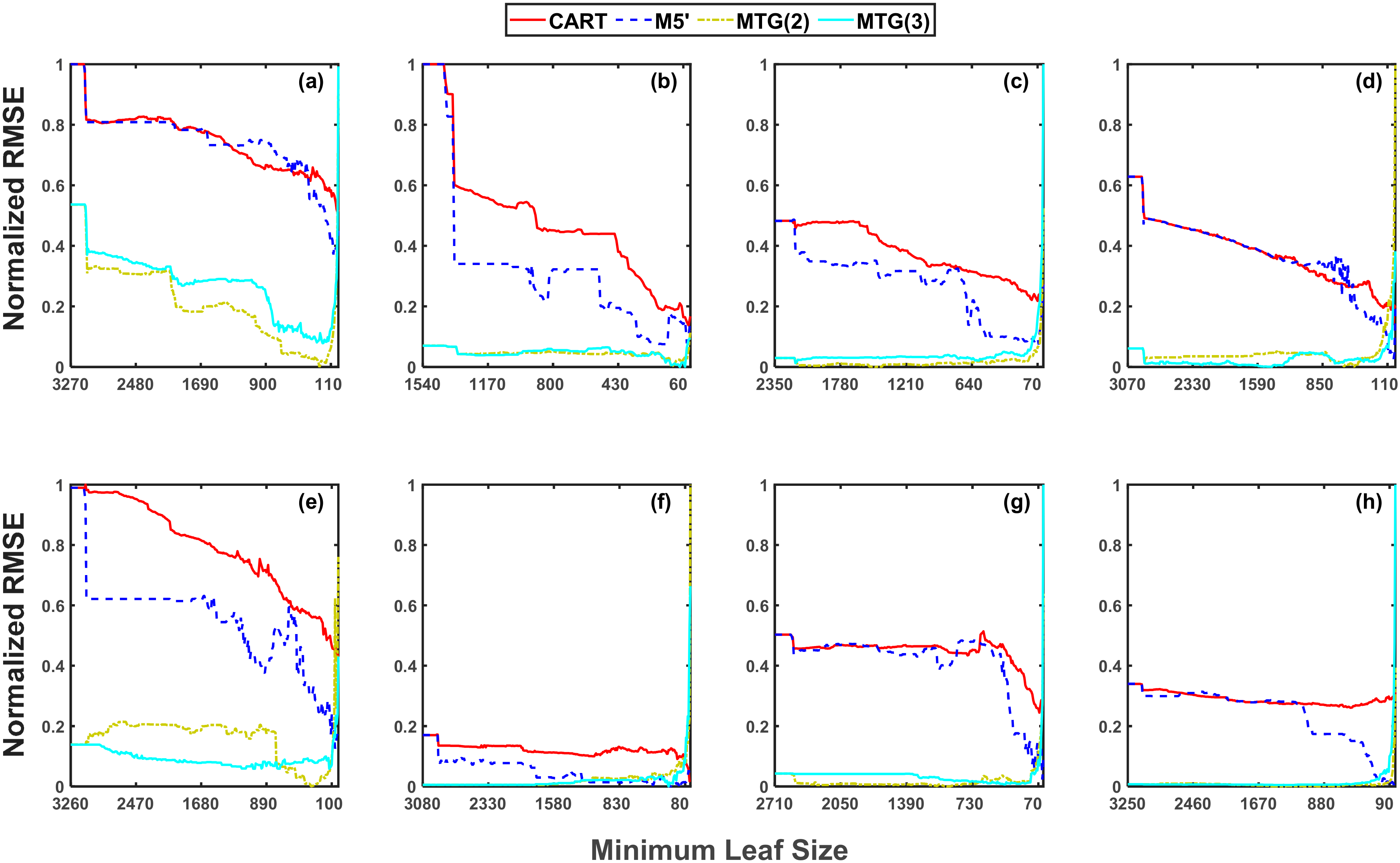
Similar to the machine learning case studies, we start our analysis by finding the best setting for MTG, CART, and M5′. We employ three combinations of settings as shown in Table 3 to find the minimum leaf size for MTG algorithm. Figure 9 shows the normalized RMSE values of daily discharge against the minimum leaf size for CART, M5′, MTG(2), and MTG(3) for validation data. Since the performance of the MTG(1) and MTG(2) was observed to be very similar, we only use MTG(2) for this analysis. According to Figure 9, in most cases the normalized RMSE values of models generated by MTG are lower than CART and M5′. The performance of the MTG on the validation data shows that the PCA dimension reduction method has slightly affected the performance of the resulted models in some cases. This behavior is similar to the machine learning case studies. The RMSE values are employed to find the minimum leaf size setting for each of the algorithms. Table 5 lists the minimum leaf size for each of the algorithms. It is evident that the minimum leaf size for the MTG algorithm is larger than that of the CART and M5′ algorithm. This indicates that the best performing inducted models by MTG are shallower and have smaller depth in comparison to CART and M5′. It should be noted that in some cases models generated by M5′ has fewer number of branches than MTG, as M5′ prune the resulted models. The minimum leaf size obtained from our analysis are employed to evaluate the models.

4. Results

4.1. Machine Learning Datasets

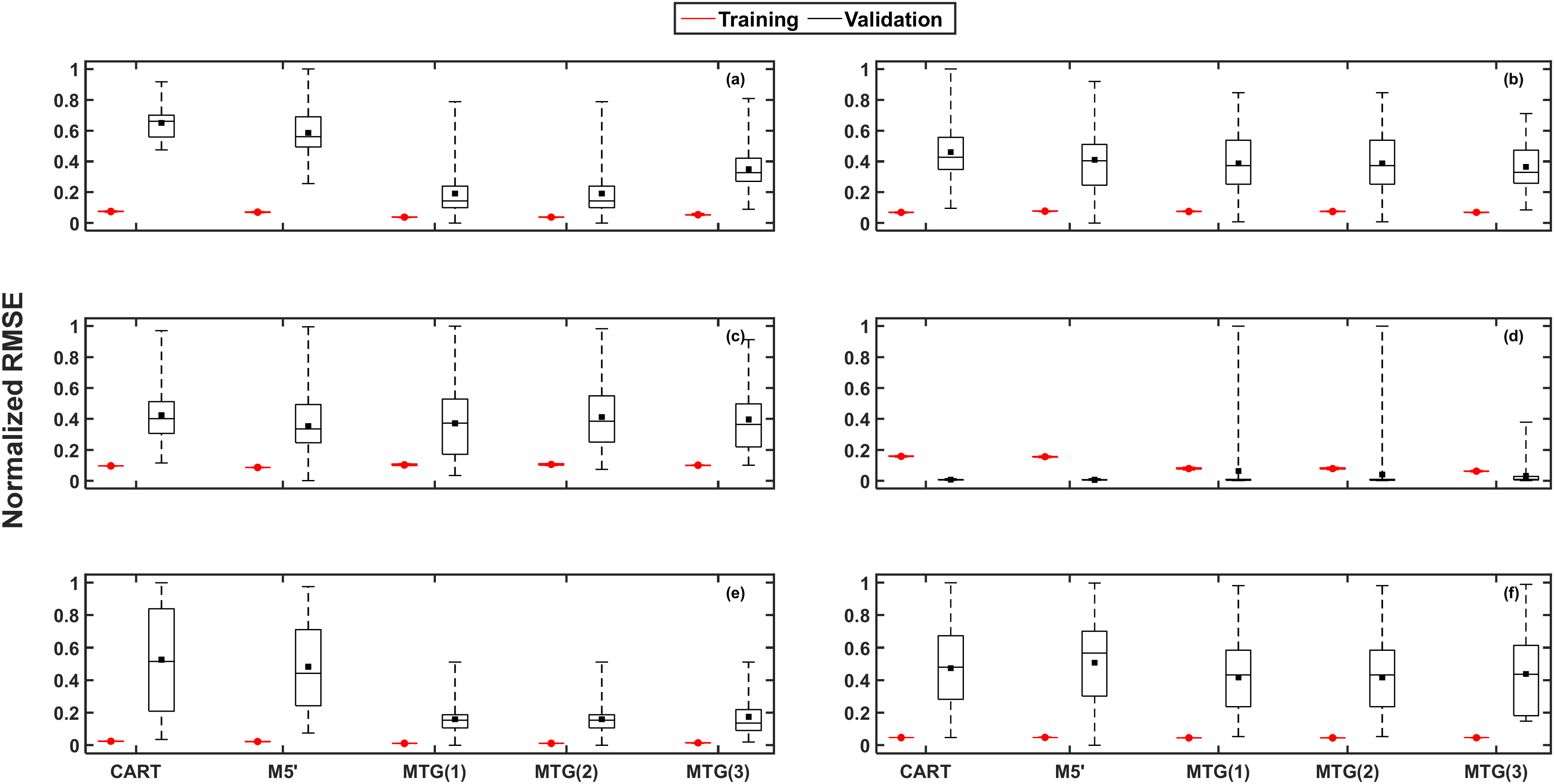
In this section, we evaluate the performance of the MTG framework along with CART and M5′ on the selected case studies. We perform a KCV with 30 folds using the settings and minimum leaf size from our analysis. Figure 10 shows the normalized RMSE values for the training data set for the cross-validation in red. In most cases, MTG(1) and MTG(2) shows superior performance over training data, except for case (c). The superior performance of the MTG is due to the regressed lines employed in the terminal nodes. The effect of the SSRML on the performance of the inducted models was also shown in the analysis in the previous section. As shown in the previous section, the quantile sampling module has no effect on the performance of the resulted models, which is also reflected in this figure. The PCA dimension reduction method has slightly increased RMSE values in most cases, as expected.
Figure 10 also shows the normalized RMSE values for the validation data for the case studies in black. These results show that MTG with SSRML is superior to other methods in almost all cases, except case (c). The performance of the inducted models on the case studies shows that MTG with PCA dimension reduction has inferior performance in comparison to other settings of the MTG algorithm. Hence, the dimension reduction approach is more suitable for the large datasets that speed enhancement is necessary. The comparison of the induction speed is not presented for the machine learning case studies as the size of these datasets cannot demonstrate the benefit of the implemented modules. The presented cases are solely employed to show the effect of the new induction approaches on the performance of the inducted models. The effects of the speed enhancement modules are further discussed on the reservoir case studies.

4.2. Reservoir Routing

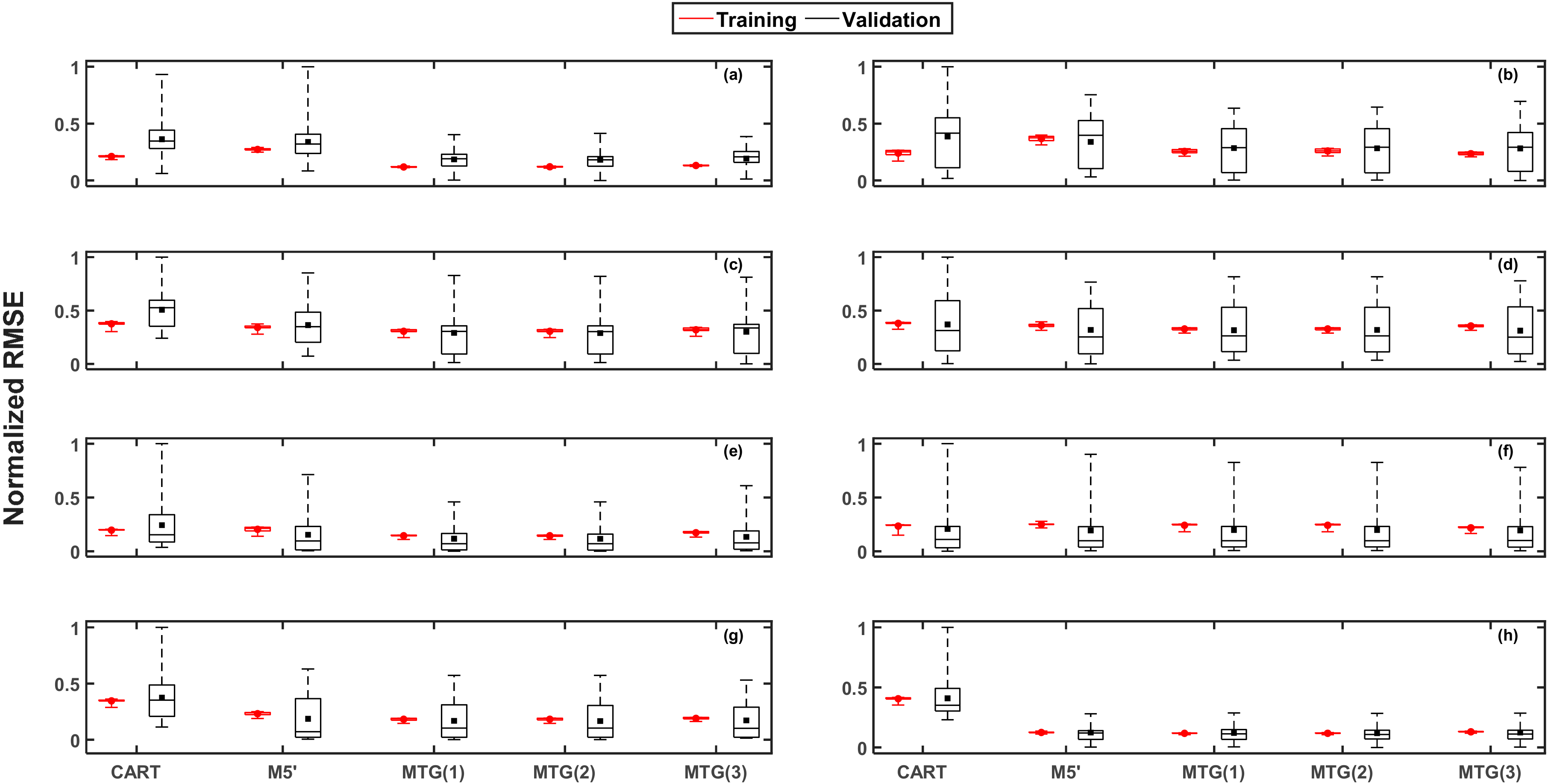
The settings from the analysis section are employed to evaluate the performance of the algorithms. Figure 11 shows the normalized RMSE values of daily discharge for the training (in red) and validation (in black) data for KCV, where each year of data is treated as a fold in KCV. This way, each fold of data consists both low and high flows. The results show that the models inducted by the MTG framework has lower median and mean RMSE values for both training and validation data. This shows the effectiveness of the default settings for a wide range of datasets. On the other hand, the PCA approach has deteriorated the performance in some cases. However, the performance of the MTG with PCA is still better than CART and M5′ in most cases. Among all the presented models, models generated by CART algorithm are inferior to others in almost all the cases. The reason for the poor performance of the CART algorithm is the constant terminal node values. Since reservoir dataset is a continuous data, the CART algorithm cannot capture the variability of these systems. It is worth noting that the CART algorithm can capture low flows in many cases as the algorithm assumes constant values for these flows. On the other hand, the MT induction algorithms (M5′ and MTG) can generate models which better describe the variability of these systems. In some cases, the validation error is smaller than the training error. This is due to the variability of extreme flows during the whole training and validation period (like a dry validation period).
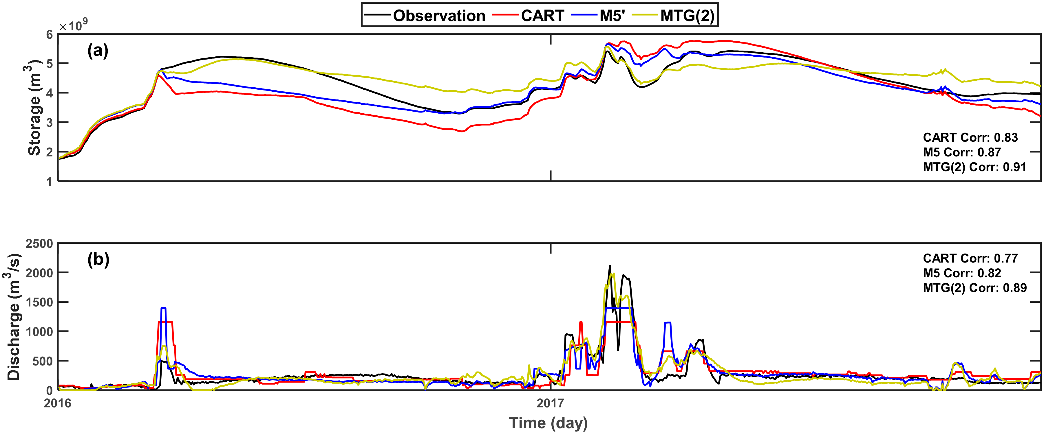
Table 2 setting for the MTG framework, as it was observed to provide the best performance with an efficient induction approach. We use 2016 and 2017 as the testing years, as there are multiple peaks in these years, and the rest of data for training. In this example, a mass balance equation is employed to derive the storage volume of Shasta reservoir using the reservoir routing models as follows,
S t = S t 1 + I t R t ,
where S t , I t and R t are the storage, inflow, and discharge volume at time t , respectively. The derived storage volume is then used as an input to the model to calculate discharge for the next step (as input to the models). This way we can observe the propagation of error during the simulation period. Figure 12 shows the simulated storage (top plot) and discharge (bottom plot) for Shasta reservoir for CART, M5′, and MTG(2). According to Figure 12, MTG(2) can better capture the peak flows and variability of data. Although the peaks are well simulated by MTG(2), the model over-estimated low flows at the end of the period, due to the high inflow values. Similar behavior is observed for the M5′ algorithm. This can also be observed in the beginning of 2016 for all the model. However, MTG(2) shows better performance for the whole period, specifically for the peak flows. The model generated by CART uses constant values for flows and shows less variability for most flows. These results support the application of the MTs for reservoir routing and efficiency and effectiveness of the MTG framework for generating these types of models. Furthermore, the storage derived by the generated discharge with MTG model can better capture the variability of the storage for the whole period, in comparison to CART and M5′ algorithms. This is also evident from the correlation between the simulated and observed discharge and storage for the MTG(2) model.

4.3. Induction Speed of the MTG Framework

The MTG framework is equipped with a quantile sampling and dimension reduction mechanism to enhance the induction speed of MTs. The quantile sampling mechanism can significantly reduce the number of split candidates, while covering the range of values for each explanatory variable. Considering a node with D attributes and N instances, the size of data in the node will be D × N . If the minimum leaf size is set to μ, the number of candidates’ cut points in an exhaustive search process will be N 2 × μ 1 × D . In most cases μ N (nodes closer to the root node have more instances). Hence, the exhaustive search mechanism evaluates all the N 2 × μ 1 × D candidates. Therefore, induction time has a direct relationship with the dimension of data in each node. The equidistant quantile sampling scheme can significantly reduce the number of splitting candidates at each node. The number of splitting candidates in this process is ρ × D where ρ is the number of equidistant quantile candidates for each dimension. Applying the default setting of the algorithm ( ρ = 100 ), MTG evaluates 100 × D candidates at each node which is smaller than the exhaustive search method in most cases. The PCA dimension reduction, on the other hand, reduces the number of attributes employed for linear regression at each node. Since SSRML employs linear regression to find the best variable and cut point, PC regression can significantly enhance the induction speed of these type of models for datasets with a large number of attributes.
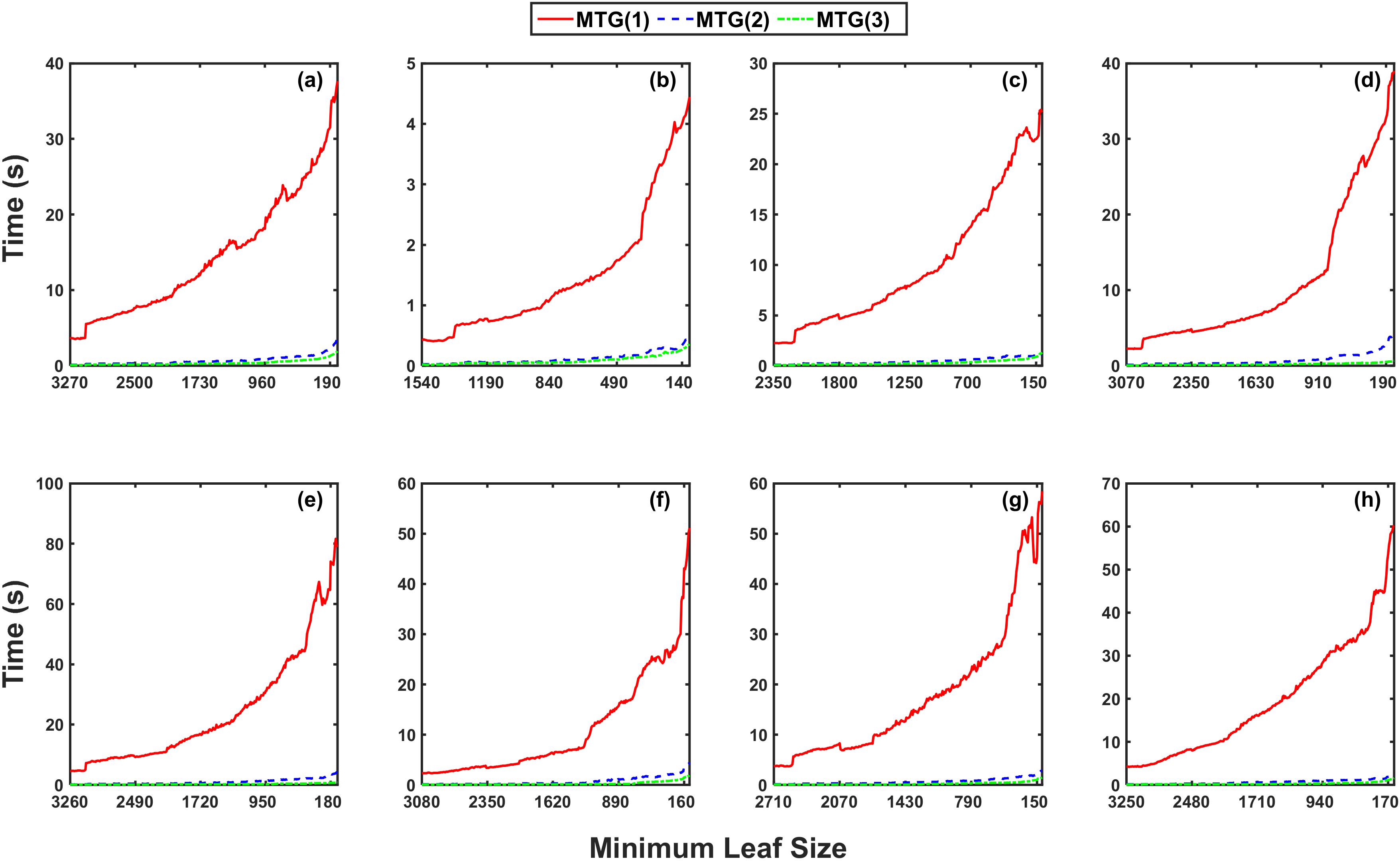
Here, we compare the induction speed of MTs for MTG(1), MTG(2) and MTG(3). We only compare these three settings as CART and M5′ are developed in different programming language and different toolboxes. Figure 13 shows the induction time of the models for different minimum leaf size values for MTG(1), MTG(2) and MTG(3). The figure shows that the quantile sampling method can significantly reduce the induction time of MTs. This shows the effectiveness of the module for reducing the induction speed of MTs, while maintaining the accuracy of the models. On the other hand, the dimension reduction component has slightly reduced the induction time for reservoir cases. The dimension reduction module is less effective in comparison to the quantile sampling module as the number of attributes for these datasets is limited to eight. The effect of this module would be more significant on datasets with larger number of attributes. Also, decreasing the minimum leaf size has less effect on the induction speed of the MTG(2) and MTG(3), which shows the effectiveness of these modules on inducting deep trees. This feature also enables generating a large number of MTs for ensemble models.

5. Conclusions

In this paper, a new decision tree induction framework, titled Model Tree Generator (MTG) is introduced. The proposed framework provides a fast, flexible, and robust model tree induction algorithm for growing MTs. The new framework can employ different SC for MT induction, which results in a different structure for the inducted models. In addition, the framework employs two different modules to enhance the induction speed of the algorithm, while it maintains the performance and accuracy of the inducted models. These modules include a quantile sampling method, which reduces the number of candidates for cut points, and local dimension reduction, which reduces the number of attributes for more complex SC. These two modules can significantly reduce the computational burden of the induction methods, which makes them suitable for large datasets with large number of attributes and instances.
We first tested the framework on six machine learning case studies. Our experiment revealed the effect of the splitting criterion on the performance of the resulted models. We showed that considering linear regression during the tree induction approaches can enhance the performance of the resulted MTs. We used this finding to suggest the default settings for the MTG framework, which can be applied to a wide range of datasets. We further tested the new framework on eight reservoirs to simulate the controlled discharge from these systems. We employed CART and M5′ algorithms as the benchmark algorithms to evaluate the performance of the default settings of the MTG framework. Since the minimum leaf size is the most important controlling parameter in these algorithms, we performed a sensitivity analysis to find the best leaf size value for all case studies and algorithms.
In addition, we showed that MTs leverage their simplicity to the multiple linear regression models employed in the terminal nodes. Hence, MTs can be easily used and combined with other models. This feature allows implementing the inducted MTs into any programming languages without the need for external libraries and complex functions. The efficiency of the MTG framework, along with the performance of the MTs makes MTG a robust candidate for representing any system within the hydrologic models. Furthermore, the performance of the algorithm on the reservoir case studies supports the application of MTs for reservoir routing. The MTs generated by MTG framework can also provide useful information about the underlying process. This allows us to understand, audit and modify these models.
Nonetheless, this paper serves as an introduction to the MTG framework. Hence, there are potential directions for employing and improving the framework. Although, the presented results support the performance of the algorithm on different datasets, there are multiple areas for future investigations. In most hydrologic systems, physical constraints can play a significant role in the performance of the models. These constraints can specifically control the model output, especially for unseen data and extrapolated values, to avoid unrealistic simulations. These constraints can be combined with the inducted MTs to further enhance the performance of these models. In addition, the potential application of the MTs in hydrologic models needs further investigation. The output of the MTG framework can be integrated within large scale hydrologic models for reservoir routing to address the effect of reservoir operation in the river systems, and to improve the modeling results. However, the potential application of the MTG framework for reservoir routing requires coupling the generated models with a hydrologic model. Furthermore, employing other hydrologic variables can further enhance the performance of models for reservoir routing. The speed enhancement modules allow MTG to train several MTs for a dataset to be used in an ensemble form, which could further improve the performance of the resulted model. Finally, the dimension reduction module employed here may remove information from the dataset due to the nature of PCA. MTG allows employing other dimension reduction approaches at the node scale, which can improve the induction speed without deteriorating the performance of the resulted models.

Author Contributions

Conceptualization, M.R.N., K.-l.H., T.Y., B.A.; software, M.R.N.; investigation, M.R.N., K.-l.H., B.A.; data curation and processing, A.T., M.R.N.; writing—original draft preparation, M.R.N.; writing—review and editing, S.S., K.-l.H., A.A., T.Y., A.T., B.A.; visualization, M.R.N.; resources, S.S., K.-l.H.; supervision, S.S., K.-l.H., A.A.; funding acquisition, S.S., K.-l.H. All authors have read and agreed to the published version of the manuscript.

Funding

This work is supported by U.S. Department of Energy (DOE Prime Award # DE-IA0000018), California Energy Commission (CEC Award # 300-15-005), NASA Minority University Research and Education Project (MIRO NNX15AQ06A) and office of vice chancellor for research, UC, Irvine.

Acknowledgments

Machine learning data is obtained from UCI Machine Learning Repository. Data on lakes and reservoirs were obtained from U.S. Army Engineer Research and Development Center and California Data Exchange Center (CDEC). The M5′ code is obtained from Gints Jekabsons website.

Conflicts of Interest

The authors declare no conflict of interest.

References

  1. Afzali Gorooh, V.; Kalia, S.; Nguyen, P.; Hsu, K.; Sorooshian, S.; Ganguly, S.; Nemani, R.R. Deep Neural Network Cloud-Type Classification (DeepCTC) model and its application in evaluating PERSIANN-CCS. Remote Sens. 2020, 12, 316. [Google Scholar] [CrossRef] [Green Version]
  2. Sadeghi, M.; Asanjan, A.A.; Faridzad, M.; Nguyen, P.; Hsu, K.; Sorooshian, S.; Braithwaite, D. PERSIANN-CNN: Precipitation estimation from remotely sensed information using artificial neural networks–convolutional neural networks. J. Hydrometeorol. 2019, 20, 2273–2289. [Google Scholar] [CrossRef]
  3. Akbari Asanjan, A.; Yang, T.; Hsu, K.; Sorooshian, S.; Lin, J.; Peng, Q. Short-Term precipitation forecast based on the PERSIANN system and LSTM recurrent neural networks. J. Geophys. Res. Atmos. 2018, 123, 12,512–543,563. [Google Scholar] [CrossRef]
  4. Zhang, D.; Lin, J.; Peng, Q.; Wang, D.; Yang, T.; Sorooshian, S.; Liu, X.; Zhuang, J. Modeling and simulating of reservoir operation using the artificial neural network, support vector regression, deep learning algorithm. J. Hydrol. 2018, 565, 720–736. [Google Scholar] [CrossRef] [Green Version]
  5. Etemad-Shahidi, A.; Taghipour, M. Predicting longitudinal dispersion coefficient in natural streams using M5′ model tree. J. Hydraul. Eng. 2012, 138, 542–554. [Google Scholar] [CrossRef]
  6. Jung, N.-C.; Popescu, I.; Kelderman, P.; Solomatine, D.P.; Price, R.K. Application of model trees and other machine learning techniques for algal growth prediction in Yongdam reservoir, Republic of Korea. J. Hydroinformatics 2009, 12, 262–274. [Google Scholar] [CrossRef] [Green Version]
  7. Guidotti, R.; Monreale, A.; Ruggieri, S.; Turini, F.; Giannotti, F.; Pedreschi, D. A survey of methods for explaining black box models. ACM Comput. Surv. 2018, 51, 1–42. [Google Scholar] [CrossRef] [Green Version]
  8. Ciampi, A. Generalized regression trees. Comput. Stat. Data Anal. 1991, 12, 57–78. [Google Scholar] [CrossRef]
  9. De’ath, G.; Fabricius, K.E. Classification and regression trees: A powerful yet simple technique for ecological data analysis. Ecology 2000, 81, 3178–3192. [Google Scholar] [CrossRef]
  10. Loh, W. Fifty years of classification and regression trees. Int. Stat. Rev. 2014, 82, 329–348. [Google Scholar] [CrossRef] [Green Version]
  11. Friedl, M.A.; Brodley, C.E. Decision tree classification of land cover from remotely sensed data. Remote Sens. Environ. 1997, 61, 399–409. [Google Scholar] [CrossRef]
  12. Huang, C.; Townshend, J.R.G. A stepwise regression tree for nonlinear approximation: Applications to estimating subpixel land cover. Int. J. Remote Sens. 2003, 24, 75–90. [Google Scholar] [CrossRef]
  13. Pal, M.; Mather, P.M. An assessment of the effectiveness of decision tree methods for land cover classification. Remote Sens. Environ. 2003, 86, 554–565. [Google Scholar] [CrossRef]
  14. Castelletti, A.; Galelli, S.; Restelli, M.; Soncini-Sessa, R. Tree-based reinforcement learning for optimal water reservoir operation. Water Resour. Res. 2010, 46, W09507. [Google Scholar] [CrossRef]
  15. Yang, T.; Gao, X.; Sorooshian, S.; Li, X. Simulating California reservoir operation using the classification and regression-tree algorithm combined with a shuffled cross-validation scheme. Water Resour. Res. 2016, 52, 1626–1651. [Google Scholar] [CrossRef] [Green Version]
  16. Yang, T.; Asanjan, A.A.; Welles, E.; Gao, X.; Sorooshian, S.; Liu, X. Developing reservoir monthly inflow forecasts using artificial intelligence and climate phenomenon information. Water Resour. Res. 2017, 53, 2786–2812. [Google Scholar] [CrossRef]
  17. Herman, J.D.; Giuliani, M. Policy tree optimization for threshold-based water resources management over multiple timescales. Environ. Model. Softw. 2018, 99, 39–51. [Google Scholar] [CrossRef]
  18. Yang, T.; Liu, X.; Wang, L.; Bai, P.; Li, J. Simulating hydropower discharge using multiple decision tree methods and a dynamical model merging technique. J. Water Resour. Plan. Manag. 2020, 146, 4019072. [Google Scholar] [CrossRef]
  19. Galelli, S.; Castelletti, A. Assessing the predictive capability of randomized tree-based ensembles in streamflow modelling. Hydrol. Earth Syst. Sci. 2013, 17, 2669–2684. [Google Scholar] [CrossRef] [Green Version]
  20. Han, J.; Mao, K.; Xu, T.; Guo, J.; Zuo, Z.; Gao, C. A soil moisture estimation framework based on the CART algorithm and its application in China. J. Hydrol. 2018, 563, 65–75. [Google Scholar] [CrossRef]
  21. Wang, Y.; Witten, I.H. Induction of Model Trees for Predicting Continuous Classes; University of Waikato: Hamilton, New Zealand, 1996. [Google Scholar]
  22. Breiman, L. Classification and Regression Trees; Routledge: New York, NY, USA, 2017; ISBN 1351460498. [Google Scholar]
  23. Malerba, D.; Esposito, F.; Ceci, M.; Appice, A. Top-down induction of model trees with regression and splitting nodes. IEEE Trans. Pattern Anal. Mach. Intell. 2004, 26, 612–625. [Google Scholar] [CrossRef] [PubMed] [Green Version]
  24. Etemad-Shahidi, A.; Mahjoobi, J. Comparison between M5′ model tree and neural networks for prediction of significant wave height in Lake Superior. Ocean Eng. 2009, 36, 1175–1181. [Google Scholar] [CrossRef]
  25. Quinlan, J.R. Learning with continuous classes. In Proceedings of the 5th Australian Joint Conference on Artificial Intelligence, Hobart, Tasmania, 16–18 November 1992; World Scientific: Singapore; Volume 92, pp. 343–348. [Google Scholar]
  26. Elshorbagy, A.; Corzo, G.; Srinivasulu, S.; Solomatine, D.P. Experimental investigation of the predictive capabilities of data driven modeling techniques in hydrology-Part 1: Concepts and methodology. Hydrol. Earth Syst. Sci. 2010, 14, 1931–1941. [Google Scholar] [CrossRef] [Green Version]
  27. Elshorbagy, A.; Corzo, G.; Srinivasulu, S.; Solomatine, D.P. Experimental investigation of the predictive capabilities of data driven modeling techniques in hydrology-Part 2: Application. Hydrol. Earth Syst. Sci. 2010, 14, 1943–1961. [Google Scholar] [CrossRef] [Green Version]
  28. Galelli, S.; Castelletti, A. Tree-based iterative input variable selection for hydrological modeling. Water Resour. Res. 2013, 49, 4295–4310. [Google Scholar] [CrossRef]
  29. Jothiprakash, V.; Kote, A.S. Effect of pruning and smoothing while using M5 model tree technique for reservoir inflow prediction. J. Hydrol. Eng. 2011, 16, 563–574. [Google Scholar] [CrossRef]
  30. Kompare, B.; Steinman, F.; Cerar, U.; Dzeroski, S. Prediction of rainfall runoff from catchment by intelligent data analysis with machine learning tools within the artificial intelligence tools. Acta Hydrotech. 1997, 16, 79–94. [Google Scholar]
  31. Rezaie-balf, M.; Naganna, S.R.; Ghaemi, A.; Deka, P.C. Wavelet coupled MARS and M5 Model Tree approaches for groundwater level forecasting. J. Hydrol. 2017, 553, 356–373. [Google Scholar] [CrossRef]
  32. Solomatine, D.P.; Dulal, K.N. Model trees as an alternative to neural networks in rainfall—runoff modelling. Hydrol. Sci. J. 2003, 48, 399–411. [Google Scholar] [CrossRef]
  33. Štravs, L.; Brilly, M. Development of a low-flow forecasting model using the M5 machine learning method. Hydrol. Sci. J. 2007, 52, 466–477. [Google Scholar] [CrossRef]
  34. Bhattacharya, B.; Solomatine, D.P. Neural networks and M5 model trees in modelling water level–discharge relationship. Neurocomputing 2005, 63, 381–396. [Google Scholar] [CrossRef]
  35. Witten, I.H.; Frank, E. Data mining: Practical machine learning tools and techniques with Java implementations. ACM Sigmod Rec. 2002, 31, 76–77. [Google Scholar] [CrossRef]
  36. Elomaa, T.; Rousu, J. General and efficient multisplitting of numerical attributes. Mach. Learn. 1999, 36, 201–244. [Google Scholar] [CrossRef]
  37. Yang, T.; Asanjan, A.A.; Faridzad, M.; Hayatbini, N.; Gao, X.; Sorooshian, S. An enhanced artificial neural network with a shuffled complex evolutionary global optimization with principal component analysis. Inf. Sci. 2017, 418, 302–316. [Google Scholar] [CrossRef] [Green Version]
  38. Chen, K.; Guo, S.; Wang, J.; Qin, P.; He, S.; Sun, S.; Naeini, M.R. Evaluation of GloFAS-Seasonal Forecasts for Cascade Reservoir Impoundment Operation in the Upper Yangtze River. Water 2019, 11, 2539. [Google Scholar] [CrossRef] [Green Version]
  39. Gaddam, S.R.; Phoha, V.V.; Balagani, K.S. K-Means+ ID3: A novel method for supervised anomaly detection by cascading K-Means clustering and ID3 decision tree learning methods. IEEE Trans. Knowl. Data Eng. 2007, 19, 345–354. [Google Scholar] [CrossRef]
  40. Laurent, H.; Rivest, R.L. Constructing optimal binary decision trees is NP-complete. Inf. Process. Lett. 1976, 5, 15–17. [Google Scholar]
  41. Ishwaran, H. Variable importance in binary regression trees and forests. Electron. J. Stat. 2007, 1, 519–537. [Google Scholar] [CrossRef]
  42. Murthy, S.K.; Salzberg, S. Decision Tree Induction: How Effective Is the Greedy Heuristic? In Proceedings of the KDD, Montreal, Canada, 20–21 August 1995; pp. 222–227. [Google Scholar]
  43. Hazen, A. Storage to be provided in impounding reservoirs for municipal water supply. Proc. Am. Soc. Civil Eng. 1914, 39, 1943–2044. [Google Scholar]
  44. Cunnane, C. Unbiased plotting positions—A review. J. Hydrol. 1978, 37, 205–222. [Google Scholar] [CrossRef]
  45. Rahnamay Naeini, M.; Analui, B.; Gupta, H.V.; Duan, Q.; Sorooshian, S. Three decades of the Shuffled Complex Evolution (SCE-UA) optimization algorithm: Review and applications. Sci. Iran. 2019, 26, 2015–2031. [Google Scholar]
  46. Rahnamay Naeini, M.; Yang, T.; Sadegh, M.; AghaKouchak, A.; Hsu, K.-L.; Sorooshian, S.; Duan, Q.; Lei, X. Shuffled Complex-Self Adaptive Hybrid EvoLution (SC-SAHEL) optimization framework. Environ. Model. Softw. 2018, 104. [Google Scholar] [CrossRef] [Green Version]
  47. Hsu, K.; Gupta, H.V.; Gao, X.; Sorooshian, S.; Imam, B. Self-organizing linear output map (SOLO): An artificial neural network suitable for hydrologic modeling and analysis. Water Resour. Res. 2002, 38, 31–38. [Google Scholar] [CrossRef] [Green Version]
  48. Shlens, J. A tutorial on principal component analysis. arXiv 2014, arXiv:1404.1100x51. [Google Scholar]
  49. Jolliffe, I.T. A note on the use of principal components in regression. J. R. Stat. Soc. Ser. C (Appl. Stat.) 1982, 31, 300–303. [Google Scholar] [CrossRef]
  50. Broman, K.W.; Speed, T.P. A model selection approach for the identification of quantitative trait loci in experimental crosses. J. R. Stat. Soc. Ser. B (Stat. Methodol.) 2002, 64, 641–656. [Google Scholar] [CrossRef]
  51. Schwarz, G. Estimating the dimension of a model. Ann. Stat. 1978, 6, 461–464. [Google Scholar] [CrossRef]
  52. Diks, C.G.H.; Vrugt, J.A. Comparison of point forecast accuracy of model averaging methods in hydrologic applications. Stoch. Environ. Res. Risk Assess. 2010, 24, 809–820. [Google Scholar] [CrossRef] [Green Version]
  53. Sadegh, M.; Ragno, E.; AghaKouchak, A. Multivariate C opula A nalysis T oolbox (MvCAT): Describing dependence and underlying uncertainty using a B ayesian framework. Water Resour. Res. 2017, 53, 5166–5183. [Google Scholar] [CrossRef]
  54. Nasta, P.; Vrugt, J.A.; Romano, N. Prediction of the saturated hydraulic conductivity from Brooks and Corey’s water retention parameters. Water Resour. Res. 2013, 49, 2918–2925. [Google Scholar] [CrossRef] [Green Version]
  55. Asuncion, A.; Newman, D. UCI Machine Learning Repository. 2007. Available online: http://archive.ics.uci.edu/ml (accessed on 30 June 2020).
  56. Mehran, A.; Mazdiyasni, O.; AghaKouchak, A. A hybrid framework for assessing socioeconomic drought: Linking climate variability, local resilience, and demand. J. Geophys. Res. Atmos. 2015, 120, 7520–7533. [Google Scholar] [CrossRef]
  57. Simonovic, S.P. Reservoir systems analysis: Closing gap between theory and practice. J. Water Resour. Plan. Manag. 1992, 118, 262–280. [Google Scholar] [CrossRef]
  58. Castillo-Botón, C.; Casillas-Pérez, D.; Casanova-Mateo, C.; Moreno-Saavedra, L.M.; Morales-Díaz, B.; Sanz-Justo, J.; Salcedo-Sanz, P.A. Analysis and Prediction of dammed water level in a hydropower reservoir using machine learning and persistence-based techniques. Water 2020, 12, 1528. [Google Scholar] [CrossRef]
  59. Ahmad, A.; El-Shafie, A.; Razali, S.F.M.; Mohamad, Z.S. Reservoir optimization in water resources: A review. Water Resour. Manag. 2014, 28, 3391–3405. [Google Scholar] [CrossRef]
  60. Rahnamay Naeini, M. A Framework for Optimization and Simulation of Reservoir Systems Using Advanced Optimization and Data Mining Tools. Ph.D. Thesis, University of California Irvine, Irvine, CA, USA, 2019. [Google Scholar]
  61. Chang, F.; Chen, L.; Chang, L. Optimizing the reservoir operating rule curves by genetic algorithms. Hydrol. Process. 2005, 19, 2277–2289. [Google Scholar] [CrossRef]
  62. Draper, A.J.; Munévar, A.; Arora, S.K.; Reyes, E.; Parker, N.L.; Chung, F.I.; Peterson, L.E. CalSim: Generalized model for reservoir system analysis. J. Water Resour. Plan. Manag. 2004, 130, 480–489. [Google Scholar] [CrossRef]
  63. Oliveira, R.; Loucks, D.P. Operating rules for multireservoir systems. Water Resour. Res. 1997, 33, 839–852. [Google Scholar] [CrossRef]
  64. David, C.H.; Yang, Z.; Famiglietti, J.S. Quantification of the upstream-to-downstream influence in the Muskingum method and implications for speedup in parallel computations of river flow. Water Resour. Res. 2013, 49, 2783–2800. [Google Scholar] [CrossRef] [Green Version]
  65. Lin, P.; Pan, M.; Beck, H.E.; Yang, Y.; Yamazaki, D.; Frasson, R.; David, C.H.; Durand, M.; Pavelsky, T.M.; Allen, G.H. Global reconstruction of naturalized river flows at 2.94 million reaches. Water Resour. Res. 2019, 55, 6499–6516. [Google Scholar] [CrossRef] [Green Version]
  66. Raftery, A.E.; Madigan, D.; Hoeting, J.A. Bayesian model averaging for linear regression models. J. Am. Stat. Assoc. 1997, 92, 179–191. [Google Scholar] [CrossRef]
  67. Maidment, D.R.; Tavakoly, A.A.; David, D.R.; Yang, Z.L.; Cai, X. An upscaling process for large-scale vector-based river networks using the NHDPlus data set. In Proceedings of the Spring Speciality Conference, American Water Resources Association, New Orleans, LA, USA, 26–28 March 2012; pp. 168–173. [Google Scholar]
  68. Tavakoly, A.A.; Snow, A.D.; David, C.H.; Follum, M.L.; Maidment, D.R.; Yang, Z. Continental-scale river flow modeling of the Mississippi River Basin using high-resolution NHDPlus dataset. JAWRA J. Am. Water Resour. Assoc. 2017, 53, 258–279. [Google Scholar] [CrossRef]
  69. Yamazaki, D.; de Almeida, G.A.M.; Bates, P.D. Improving computational efficiency in global river models by implementing the local inertial flow equation and a vector-based river network map. Water Resour. Res. 2013, 49, 7221–7235. [Google Scholar] [CrossRef]
  70. Lin, P.; Yang, Z.-L.; Gochis, D.J.; Yu, W.; Maidment, D.R.; Somos-Valenzuela, M.A.; David, C.H. Implementation of a vector-based river network routing scheme in the community WRF-Hydro modeling framework for flood discharge simulation. Environ. Model. Softw. 2018, 107, 1–11. [Google Scholar] [CrossRef]
  71. Salas, F.R.; Somos-Valenzuela, M.A.; Dugger, A.; Maidment, D.R.; Gochis, D.J.; David, C.H.; Yu, W.; Ding, D.; Clark, E.P.; Noman, N. Towards real-time continental scale streamflow simulation in continuous and discrete space. JAWRA J. Am. Water Resour. Assoc. 2018, 54, 7–27. [Google Scholar] [CrossRef]
  72. Snow, A.D.; Christensen, S.D.; Swain, N.R.; Nelson, E.J.; Ames, D.P.; Jones, N.L.; Ding, D.; Noman, N.S.; David, C.H.; Pappenberger, F. A high-resolution national-scale hydrologic forecast system from a global ensemble land surface model. JAWRA J. Am. Water Resour. Assoc. 2016, 52, 950–964. [Google Scholar] [CrossRef] [Green Version]
  73. David, C.H.; Famiglietti, J.S.; Yang, Z.; Eijkhout, V. Enhanced fixed-size parallel speedup with the Muskingum method using a trans-boundary approach and a large subbasins approximation. Water Resour. Res. 2015, 51, 7547–7571. [Google Scholar] [CrossRef] [Green Version]
  74. Hejazi, M.I.; Cai, X.; Ruddell, B.L. The role of hydrologic information in reservoir operation–learning from historical releases. Adv. Water Resour. 2008, 31, 1636–1650. [Google Scholar] [CrossRef]
  75. Park, K., II. Fundamentals of Probability and Stochastic Processes with Applications to Communications; Springer: Jersey City, NJ, USA, 2018; ISBN 3319680757. [Google Scholar]
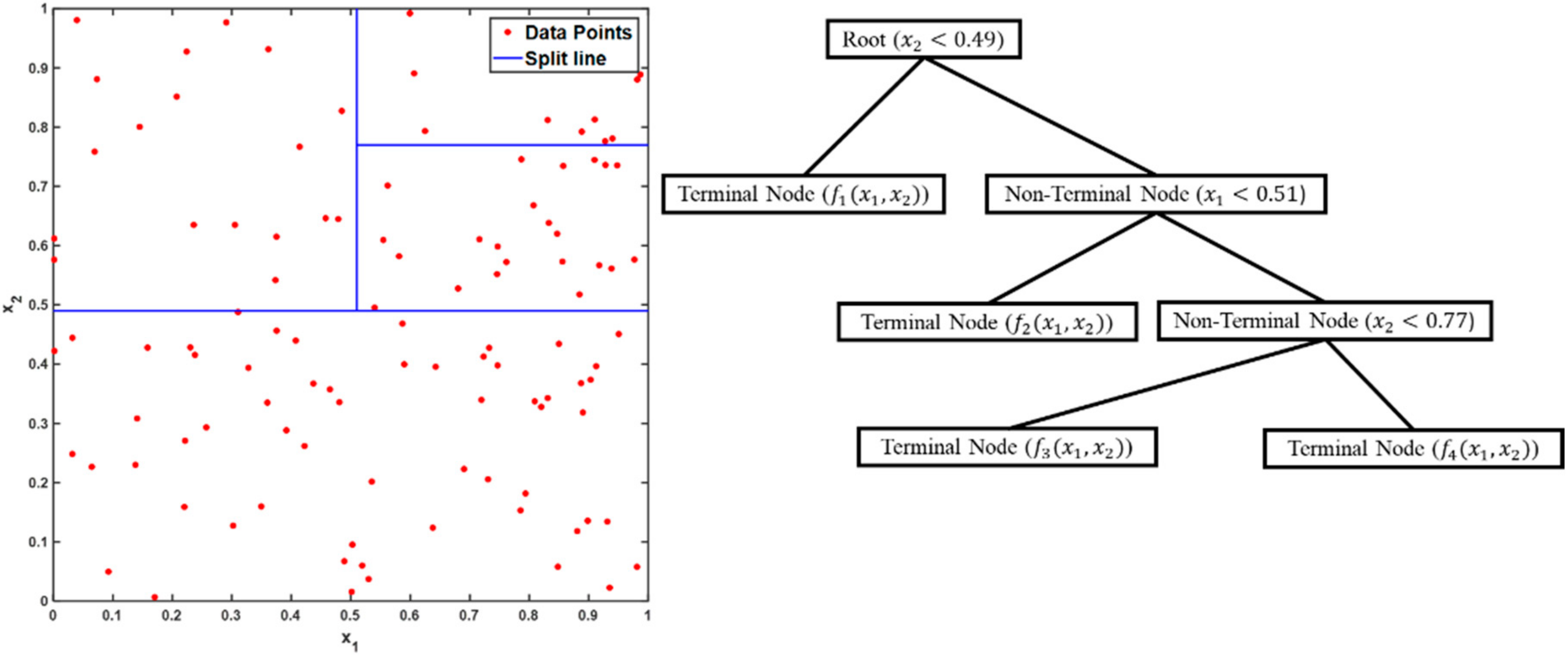
Figure 1. Representation of a binary decision tree in the independent variable space (left), and the corresponding structure of the model (right) for a synthetic data.
Water 12 02373 g001
Figure 2. The schematic representation of the binary MT induction in the MTG framework.
Water 12 02373 g002
Figure 3. A comparison between the SSRM setting with single constant values in the terminal nodes (plot A) and the SSRML setting with multiple linear regression in the terminal nodes (plot B) for generating models with the MTG framework.
Water 12 02373 g003
Figure 4. The normalized RMSE against minimum leaf size in descending order for; (a) airfoil self-noise, (b) auto MPG, (c) combined cycle power plant, (d) concrete compressive strength, (e) energy efficiency (heating load) and (f) energy efficiency (cooling load).
Water 12 02373 g004
Figure 5. The normalized RMSE against minimum leaf size in descending order for (a) airfoil self-noise, (b) Auto MPG; (c) combined cycle power plant, (d) concrete compressive Strength, (e) Energy efficiency (heating load) and (f) energy efficiency (cooling load).
Water 12 02373 g005
Figure 6. The normalized RMSE values against minimum leaf size in descending order for; (a) airfoil self-noise, (b) auto MPG, (c) combined cycle power plant; (d) concrete compressive strength, (e) energy efficiency (heating load) and (f) energy efficiency (cooling load).
Water 12 02373 g006
Figure 7. Location of the selected reservoirs over the CONUS.
Water 12 02373 g007
Figure 8. Autocorrelation of discharge data for the selected reservoirs.
Water 12 02373 g008
Figure 9. The normalized RMSE values of daily discharge against minimum leaf size in descending order for (a) Arkabutla, (b) Coralville, (c) Dale Hollow, (d) Eldorado, (e) Folsom, (f) Prado, (g) Shasta and (h) Trinity for CART, M5′, MTG(2), and MTG(3).
Water 12 02373 g009
Figure 10. Boxplots and mean values of the normalized RMSE values for; (a) airfoil self-noise, (b) Auto MPG, (c) combined cycle power plant, (d) concrete compressive strength, (e) energy efficiency (heating load) and (f) energy efficiency (cooling load) for training and validation data using the CART and M5′ algorithm and MTG framework.
Water 12 02373 g010
Figure 11. Boxplots and mean values of the normalized RMSE values of daily discharge for (a) Arkabutla, (b) Coralville, (c) Dale Hollow, (d) Eldorado, (e) Folsom, (f) Prado, (g) Shasta and (h) Trinity for training and validation data for CART, M5′, MTG(1), MTG(2), and MTG(3).
Water 12 02373 g011
Figure 12. Simulated storage; (a) and discharge (b) for Shasta dam for years 2016 and 2017 using CART, M5′, and MTG(2) algorithms.
Water 12 02373 g012
Figure 13. The induction time of models against minimum leaf size in descending order for; (a) Arkabutla, (b) Coralville, (c) Dale Hollow, (d) Eldorado, (e) Folsom, (f) Prado, (g) Shasta and (h) Trinity reservoirs for MTG(1), MTG(2), and MTG(3) on Dell XPS 8910 with core i7-6700 processor.
Water 12 02373 g013
Table 1. List of the selected UCI machine learning datasets and their size.
CaseDataset NameNo. AttributesNo. Instances
aAirfoil self-noise51503
bAuto MPG7398
cCombined cycle power plant49568
dConcrete compressive Strength81030
eEnergy efficiency (heating load)8768
fEnergy efficiency (cooling load)8768
Table 2. Minimum leaf size value for each case study and algorithm.
CaseDataset NameCARTM5′MTG (SSRML with Quantile)MTG (SSRML with Quantile and PCA)
aAirfoil self-noise10102020
bAuto MPG102010040
cCombined cycle power plant20102050
dConcrete compressive Strength10105090
eEnergy efficiency (heating load)10102030
fEnergy efficiency (cooling load)10105070
Table 3. Settings of the MTG framework.
SettingSCQuantile SamplingPCA
MTG(1)SSRML
MTG(2)SSRML×
M2G(3)SSRML ×
Table 4. List of the selected reservoirs and employed data.
CaseReservoirStateCityServicesStudy PeriodHydrologic Variables
aArkabutlaMSTunicaFlood Control, Recreation1999–2016Inflow, Pool Elevation, Discharge
bCoralvilleIAIowa CityFlood Control, Recreation2005–2013Inflow, Discharge
cDale HollowTNCelinaHydropower, Flood Control, Recreation2000–2012Inflow, Pool Elevation, Discharge
dEl DoradoKSEl DoradoFlood Control, Water Supply, Recreation2000–2016Inflow, Storage Volume, Discharge
eFolsomCAFolsomHydropower, Flood Control, Water Supply, Recreation2001–2018Inflow, Storage Volume, Discharge
fPradoCACoronaFlood Control2000–2016Inflow, Storage Volume, Discharge
gShastaCAShasta LakeHydropower, Flood Control, Water Supply, Recreation2004–2018Inflow, Storage Volume, Discharge
hTrinityCALewistonHydropower, Flood Control, Water Supply, Recreation2000–2018Inflow, Storage Volume, Discharge
Table 5. The minimum leaf size value for each case study and algorithm.
CaseReservoirCARTM5′MTG(2)MTG(3)
aArkabutla3080250210
bCoralville1016013080
cDale Hollow706014802170
dEl Dorado40404901430
eFolsom20603501030
fPrado202501660270
gShasta6030990400
hTrinity560409201470