Article

Modelling Hydrological Processes and Identifying Soil Erosion Sources in a Tropical Catchment of the Great Barrier Reef Using SWAT

1
Centre for Applied Climate Sciences, Institute for Life Sciences and the Environment, University of Southern Queensland, Toowoomba 4350, Australia
2
Centre for Sustainable Agricultural Systems, Institute for Life Sciences and the Environment, University of Southern Queensland, Toowoomba 4350, Australia
*
Author to whom correspondence should be addressed.
Water 2020, 12(8), 2179; https://doi.org/10.3390/w12082179
Submission received: 18 June 2020 / Revised: 29 July 2020 / Accepted: 30 July 2020 / Published: 2 August 2020
(This article belongs to the Section Water Erosion and Sediment Transport)

Abstract

:
Study region: North Johnstone catchment, located in the north east of Australia. The catchment has wet tropical climate conditions and is one of the major sediment contributors to the Great Barrier Reef. Study focus: The purpose of this paper was to identify soil erosion hotspots through simulating hydrological processes, soil erosion and sediment transport using the Soil and Water Assessment Tool (SWAT). In particular, we focused on predictive uncertainty in the model evaluations and presentations—a major knowledge gap for hydrology and soil erosion modelling in the context of Great Barrier Reef catchments. We carried out calibration and validation along with uncertainty analysis for streamflow and sediment at catchment and sub-catchment scales and investigated details of water balance components, the impact of slope steepness and spatio-temporal variations on soil erosion. The model performance in simulating actual evapotranspiration was compared with those of the Australian Landscape Water Balance (AWRA-L) model to increase our confidence in simulating water balance components. New hydrological insights for the region: The spatial locations of soil erosion hotspots were identified and their responses to different climatic conditions were quantified. Furthermore, a set of land use scenarios were designed to evaluate the effect of reforestation on sediment transport. We anticipate that protecting high steep slopes areas, which cover a relatively small proportion of the catchment (4–9%), can annually reduce 15–26% sediment loads to the Great Barrier Reef.

1. Introduction

The Great Barrier Reef (GBR) is the world’s largest coral reef extending over 2000 km off the Queensland coastline. During the 20th century, the landscape of GBR catchments was altered dramatically as a result of expanding sugarcane, banana and livestock production. To expand agricultural lands and improve productivity, many natural waterways were replaced by drainage systems, native vegetative cover was removed, soil structure disturbed and natural wetlands emptied [1]. Vegetation clearance rules in Queensland were minimal until the mid-2000s when the enforcement of clearing restrictions came into effect to preserve remaining forests and native vegetative cover [2]. In tropical regions of Queensland, where there is a potential for high soil erosion, it is estimated that around half of its primary rainforests (6700 km2 of 13,000 km2) have been destroyed since the beginning of European colonisation [3,4]. These anthropogenic changes in GBR catchments have amplified soil erosion, increased sediment concentrations in the reef and consequently resulted in the degradation of the coral and seagrass ecosystems, which provide food and shelter for variety of marine species [5,6,7,8,9]. Specifically, the increased build-up of sediment in downstream waterbodies of GBR tropical catchments is likely to bring more ecological issues such as shrinking habitat and interstitial spaces, hence, disturbing the behaviour and lowering the survival rate of freshwater species [10].
Effective planning for controlling pollution and applying mitigation options necessitates improvement in our understanding of hydrological processes. Until now, various modelling efforts have been carried out to simulate streamflow and sediment loads flowing to the GBR including eWater Source and its plug-in, Dynamic SedNet, that have been developed and being used as industry standards for hydrology and water quality modelling for GBR catchments [11]. However, in most cases, details of the link between hydrological processes within catchments and delivered sediment loads to the GBR, as well as the uncertainty involved in model outputs and processes are not quantified [12,13,14,15,16,17]. Incorporating quantitative measures of uncertainty in a modelling approach reduces the effect of biases in the form of epistemic errors on decision making [18,19], increases our confidence in model outputs and eventually makes the approach more reliable for incorporating into ecological risk assessment [20,21].
In this research, an advanced process-based catchment model—Soil and Water Assessment Tool (SWAT) [22]—has been applied for the first time in the context of GBR catchments for modelling hydrology and soil erosion. The model has capabilities in the spatial and temporal simulation of runoff generation, soil erosion, sediment transport, plant/vegetative growth and agricultural management practices in an integrated system, plus the availability of supporting documents and additional tools such as SWAT-CUP [23] for analysing uncertainty through inverse modelling and parallel processing. We established a SWAT model for the North Johnstone catchment (a tropical catchment in the north-east of Australia), listed as a priority catchment for controlling sediment delivery to the GBR [24]. The model is calibrated and validated for daily streamflow rate and daily sediment load at the catchment and sub-catchment scales. We obtained sediment concentration data from two independent studies for two separate periods reflecting different climatic conditions from extreme wet to extreme dry. We also carried out a parameter sensitivity analysis and quantified predictive uncertainty in model outputs for both water balance components and the soil erosion from major land uses.
Previous studies predicted that protecting degraded pastures through reforestation has the potential to increase soil water retention capacity, reduce runoff and stabilise soil, and therefore, control soil erosion and improve coral reef health [25,26,27,28,29]. In addition, recently, efforts have been made to investigate cost-effective methods of successful plant species selection for reforestation on degraded pastures in the upper section of North Johnstone catchment [30,31]. Here, we investigated four land use change scenarios for converting pasture areas to rainforests to quantify the extent to which reforestation can reduce sediment loads from the North Johnstone catchment to the GBR.

2. Material and Methods
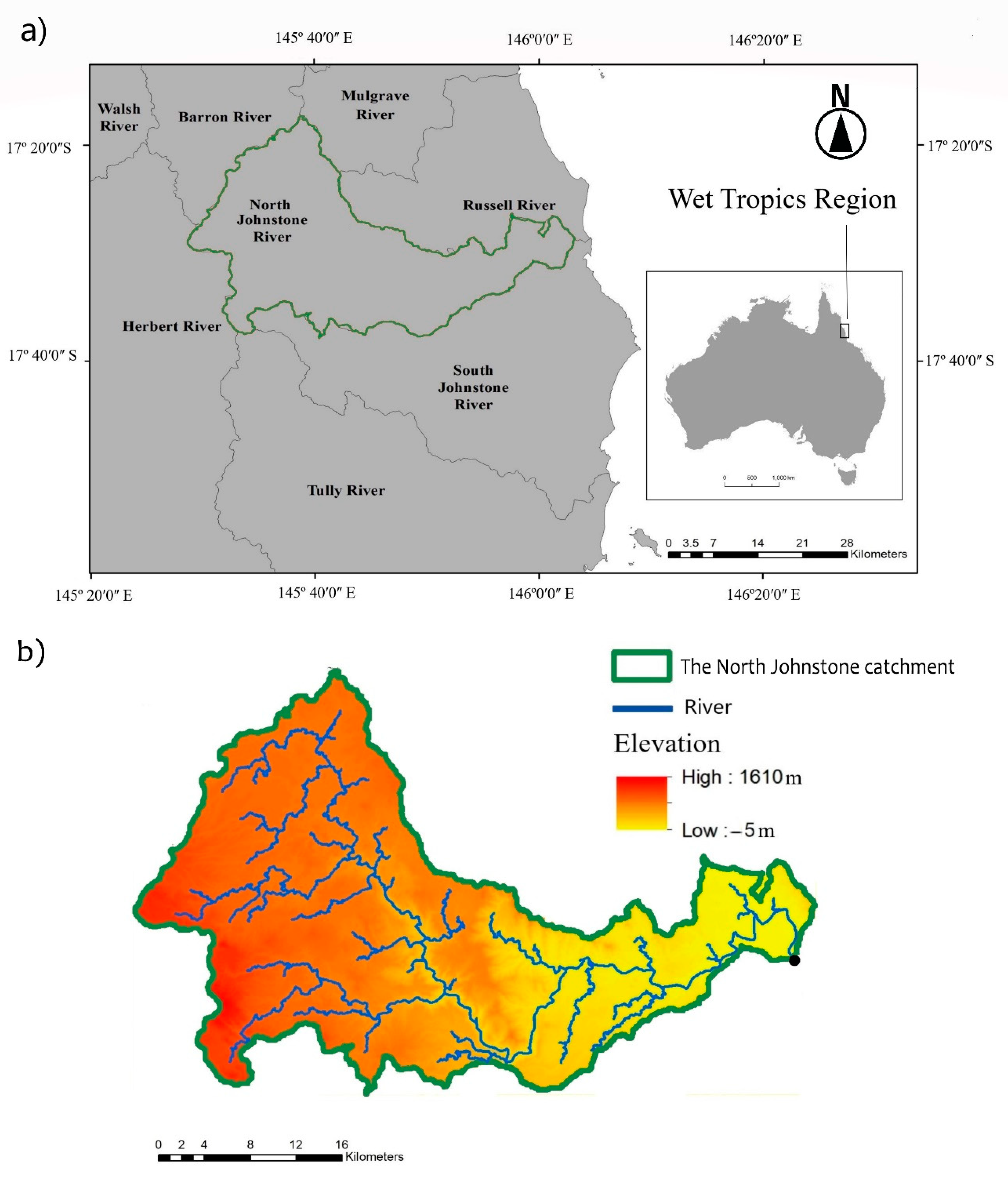
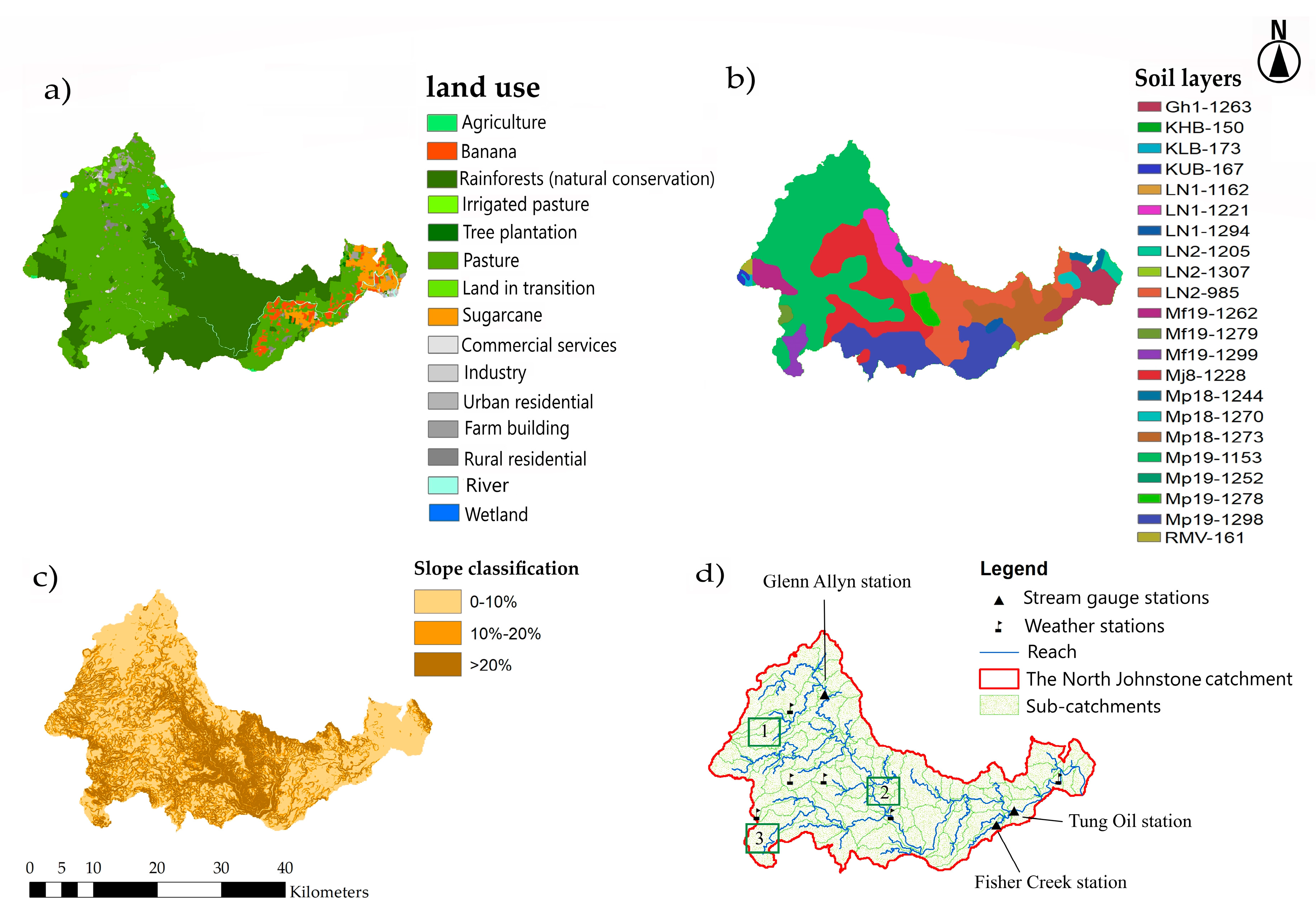
2.1. Study Area

The North Johnstone catchment is located between latitudes 17°38′ S and 17°16′ S and longitudes 145°28′ E and 146°4′ E in the Wet Tropics Region in the northeast of Australia (Figure 1). This catchment covers an area of approximately 102,980 ha.
The catchment has wet tropical climate conditions which mean that during austral summers the weather is hot, and humid with frequent and intensive rainfall while in austral winters, temperatures and rainfall are relatively low. Rainfall gradient is remarkable across the catchment; 3600 mm mean annual rainfall at the coastal areas (e.g., Innisfail) while gradually decreasing to 2000 mm mean annual rainfall towards the upper section (e.g., Malanda).
Conserved natural rainforest and pasture areas (with native or modified vegetative cover under grazing or minimal uses) cover 37% and 51% of the catchment, respectively, and thus are the dominant land uses. Agricultural farms mostly comprise bananas (2.5%) and sugarcane (3.5%) which are located in the coastal zone. A marginal proportion (less than 1%) can be attributed to tea farms and tropical fruit trees in the upper section. Other land uses are commercial/residential/industrial areas comprising 3% of the whole catchment and a small proportion is also related to the water surface and wetlands (see Figure 2a for the spatial distribution of land uses). Coastal areas have basalt and alluvium soils while the dominant soils in the upper areas are red ferrosols, dermosols and red kandosols.

2.2. Soil and Water Assessment Tool (SWAT)

SWAT is a process-based continuous daily time-step model, which enables users to simulate hydrological processes, crop growth, erosion, and pollutant transport in agricultural catchments to study the long-term impacts of the gradual build-up of pollutants on downstream water bodies [22]. SWAT has been applied successfully to various catchments with different type of environments around the world including tropical catchments in East Asia, Africa and South America [32,33,34].
SWAT is a semi-distributed model that delineates a catchment into sub-catchments and divides each sub-catchment into hydrologic response units (HRUs) based on uniform slope, land use and soil type. SWAT structure is built upon two main phases, i.e., land phase and channel phase.
In the land phase, SWAT computes water balance in each HRU and then aggregates the results to sub-catchment outputs based upon the fraction of each HRUs. SWAT calculates water balance in each HRUs based on the Equation (1).
S W t = S W 0 + i = 1 t ( R d a y Q s u r f E T a W s e e p Q g w )
where S W t is the final soil water content (mm), S W 0 is the initial soil water content on day i (mm), t is the time (days), R d a y is the amount of rainfall on day i (mm), Q s u r f is the amount of surface runoff on day i (mm), ETa is the amount of actual evapotranspiration on day i (mm), W s e e p is the amount of water entering the vadose zone from the soil profile on day i (mm) and Q g w is the amount of return flow on day i (mm).
To calculate surface runoff at daily time steps, SWAT uses the soil conservation service curve number (SCS) method [35]. The daily curve number can be calculated based on antecedent soil moisture or plant evapotranspiration of which the latter is selected for this research. For the computation of daily actual evapotranspiration, SWAT first needs to calculate potential evapotranspiration through one of the following methods: Penman–Monteith [36], Hargreaves [37] and Priestley–Taylor [38]. As wind data records are not available for the case study, potential evapotranspiration is simulated using the Priestley–Taylor method. This method requires solar radiation, air temperature and relative humidity. Further description regarding the details of the calculation of surface runoff, the movement of water in the vadose zone, ETa and groundwater recharge/discharge can be found in SWAT theoretical documentation [22].
To estimate sediment yield, SWAT employs the Modified Universal Soil Loss Equation (MUSLE, Equation (2)) [39]. While Universal Soil Loss Equation (USLE) predicts average annual gross erosion as a function of rainfall energy, in MUSLE the rainfall energy factor is replaced with a runoff factor, which improves the sediment yield prediction, eliminates the need for delivery ratios, and allows the equation to be applied to individual storm events [40]. Nevertheless, MUSLE accounts for soil losses caused by sheet, rill, and rain splash but not the erosion caused by landslides and gullies. However, only 3% of sediment loads in the whole Wet Tropic Region comes from gully erosion while 70% and 27% of sediment come, respectively, from hillslope and stream bank erosion [24].
S e d = 11.8 × ( Q s u r f · q p e a k · a r e a h r u ) 0.56 · K U S L E · C U S L E · P U S L E · L S U S L E · C F R G
where S e d is the sediment yield on a given day (t∙ha−1), Q s u r f the surface runoff volume (mm), q p e a k is the peak runoff rate (m3/s), a r e a h r u is the area of the HRU (ha), K U S L E is the MUSLE soil erodibility factor (0.013 metric ton m2 hr/(m3- metric ton cm)), C U S L E is the MUSLE cover and management factor, P U S L E is the MUSLE support practice factor, L S U S L E is the MUSLE topographic factor and CFRG is the coarse fragment factor.
In the channel phase, SWAT routes sub-catchment outputs through a river reach in the channel network to the output/s of the catchment. SWAT has five stream power equations for calculating maximum sediment concentration, modelling bank and bed erosions in a channel containing various bed materials and sediment disposition. In this study, due to the lack of data regarding the floodplain and the material of the channel bed, the simplified version of Bagnold [41] is used to calculate the maximum amount of sediment that can be transported in a stream segment. The Bagnold stream power equation calculates the maximum sediment concentration based on Equation (3) and then calculates deposition and degradation by comparing the sediment concentration in the channel and the calculated maximum sediment concentration based on Equations (4) and (5).
C o n c s e d , c h , m x = c s p · v c h ,   p k s p e x p
If
C o n c s e d ,   c h ,   i > C o n c s e d ,   c h ,   m a x     S e d d e p = ( C o n c s e d , c h , i C o n c s e d , c h , m x ) ·   V c h
If
C o n c s e d ,   c h ,   i < C o n c s e d ,   c h ,   m a x   S e d d e g = ( C o n c s e d , c h ,   m x C o n c s e d , c h , i ) ·   V c h ·   K C H · C C H
where C o n c s e d , c h , m x   is the maximum amount of sediment that can be transported (kg/L), v c h , p k is the peak channel velocity (m/s) while c s p is a coefficient (SPCON), spexp is an exponent (SPEXP), C o n c s e d , c h , i is the concentration of sediment in time step i (kg/L), K C H is the channel erodibility factor (CH_COV1), V c h is the volume of water in the reach segment (m3) and C C H is the channel cover factor (CH_COV2).

2.3. Model Input Data

Specific information regarding climate, soil properties, topography, vegetation cover and land use management practices are required by SWAT to directly simulate physical processes associated with hydrology, erosion, sediment transport and crop/plant growth for the catchment. The summary of model input data is provided in Table 1.

2.3.1. Hydrological Observation Data

Daily records of streamflow rate for the calibration period (1991–1996) and validation period (2007–2012) for three monitoring stations were obtained from the Queensland Government Water Monitoring Information portal (https://water-monitoring.information.qld.gov.au/) (see Figure 2d for the location of stream gauges).
Tung Oil station (112004A) is located at the end of the North Johnstone River receiving runoff from 92,500 ha—90% of the whole catchment. Glen Allyn (112003A) is located at the upper section of the catchment on the North Johnstone river receiving water from 16,500 ha (mostly pasture)—16% of the whole catchment. Fisher Creek Station (112002A) is located on a tributary channel receiving runoff from 1500 h—1.5% of the whole catchment—of pasture, rainforest, sugarcane and banana farms.

2.3.2. Sediment Loads Observation Data

Daily sediment concentration data for the period between 1991 and 1996 were obtained from a previous study carried out in the region by Hunter and Walton [13]; they collected sediment concentration samples in 188 days at the Tung Oil station, 149 days at the Glenn Allyn station and 113 days at Fisher Creek station. After Hunter and Walton [13], there was not any sediment monitoring until 2007 when the Queensland Department of Environment and Science started monitoring sediment concentration; however, this time only for the Tung Oil station. We used the sediment concentration data of this program for the validation period (2007–2012) in which sediment concentration samples recorded for 94 days.
To calculate sediment loads, we multiplied the average sediment concentration by the average streamflow rate of a day. Depending on the number of collected samples on a given day, this method of calculating sediment loads, like any other method, can result in underestimation or overestimation [44]. Therefore, we considered 30% error in calculated sediment loads. This error range was used for calculating P-factor described in Section 2.6.1.

2.4. Actual Evapotranspiration Database

Actual evapotranspiration (ETa) is the major mechanism of removing water from any catchment while greatly influencing water balance components of the system. We compared ETa estimation of SWAT with an external source of ETa to increase our confidence in modelling water balance components. For this purpose, we obtained ETa from the Australian Landscape Water Balance (AWRA-L) (http://www.bom.gov.au/water/landscape). AWRA-L v6 [45] is a 5 km × 5 km gridded water balance model which provides daily estimates of ETa across Australia from 2005.
We selected three locations to compare ETa including one pasture dominated area in the upper section with high altitude (765 m) and annual rainfall of 1900 mm (Figure 2d, location 1), one rainforest dominated area located in the midsection with low altitude (230 m) and high annual rainfall (3800 mm) (Figure 2d, location 2) and one mixed area of rainforest and pasture in the upper section with high altitude (1400 m) and moderate rainfall (2500 mm) (Figure 2d, location 3).

2.5. SWAT Model Setup

2.5.1. Model Setup

SWAT2012 revision 670 was applied for this research, which was the latest version available at the time. Based on the DEM map, SWAT delineated the catchment into 91 sub-catchments and finally defined 1503 HRUs based on slope classifications, soil types and land use (see Figure 2). The SWAT model was set up for daily time step with 7 years as a warm-up/equilibrium period according to recommendations by Daggupati et al. [46].

2.5.2. Parameterisation of the Vegetative Cover

Seasonal changes to the vegetative cover have a great influence on biomass production, runoff, actual evapotranspiration and soil erosion and SWAT requires specific parameters of leaf area index (LAI) of plants and crops during the growing cycle to simulate their seasonal development.
For the pasture areas, we adjusted the leaf area index (LAI) parameters of SWAT plant dataset to simulate LAI of pasture plant as much as possible close to a processed time series we retrieved from MODIS Collection 6 (MODIS15A2H) remote sensing data (http://reverb.echo.nasa.gov/) for Location 1 in the upper section of the catchment (Figure 2d). The maximum LAI of pasture plant, maximum potential biomass, and potential heat units are, respectively, considered to be 3 m2/m2, 10 t∙ha−1 and 2000.
LAI parameters of sugarcane plant are adjusted based on one study for a widely known genotype of sugarcane in Mexico with rainfed conditions [47] and two comprehensive studies for assessing and modelling yield and LAI expansion of Australian sugarcane [48,49]. The maximum LAI of sugarcane plant, maximum potential biomass, and potential heat units are, respectively, considered to be 6.5 m2/m2, 90 t∙ha−1 and 5500. We also considered one plant and two ratoons for sugarcane cultivation. Planting was considered to take place between September and November, and the first harvesting would happen in the next 12 months. For the two subsequent ratoons, we considered that harvesting would happen in the next 10 months; 90% of sugarcane biomass would be removed at ratooning events, and 10% of the removed biomass would remain on the surface as residue. Among sugarcane HRUs, different planting years are also considered to keep the heterogeneity of the time of agricultural activities in the region.
For bananas, we checked the seasonal change in LAI values with a previous study for tropical bananas [50], considering the maximum LAI up to 4.5 m2/m2, while having around 100 t∙ha−1 biomass in full maturity and gaining 30–50 t∙ha−1∙year−1 after harvesting/ratooning with potential heat units of 5500.
The LAI of the rainforest is below 5 m2/m2, which is (as a result of frequent cyclones in the region) relatively lower comparing to other rainforests across the world [51]. Thus, rainforest LAI parameters were adjusted to have a mostly consistent LAI of 4.5 m2/m2 and an average biomass of 200 t∙ha−1.

2.6. Model Calibration and Validation

2.6.1. Measuring the Model Performance

Based on suggestions by Moriasi et al. [52], two dimensionless statistical indicators—Nash Sutcliff efficiency (NSE) and the ratio of root mean square error to the standard deviation of the observations (RSR)—and one error index—percent bias (PBIAS)—were used to measure the goodness of fit of the best simulation during calibration and validation. NSE indicates a “very good” performance (for both streamflow and sediment) when it is more than 0.75 and “unsatisfactory” when it is less than 0.5; RSR indicates a “very good” performance (for both streamflow and sediment) when it is less than 0.5 and “unsatisfactory” when it is more than 0.7. However, for streamflow, when PBIAS is less than ±10%, it indicates very good performance and unsatisfactory when it is more than ±25%. For sediment loads, PBIAS less than ±15% shows a “very good” performance and “unsatisfactory” when it is more than ±55%.
We also used two indicators for evaluating the overall performance of the predictive uncertainty in model outputs including P-factor which is the percentage of observation (± error) captured by 95% prediction uncertainty (95PPU) and R-factor which is the thickness of the 95PPU envelope [53]. The range of P-factor is between 0 and 1 and the range of R-factor is between 0 and infinity. A P-factor close to 1 and R-factor less than 1 confirm the acceptable performance of the model.

2.6.2. Model Calibration

The calibration, validation, sensitivity and uncertainty analyses are carried out by employing the sequential uncertainty fitting algorithm-version 2 (SUFI-II)—an inverse modelling procedure based on Latin hypercube sampling [54] developed by Abbaspour et al. [55].
SUFI-II starts by assuming a large parameter uncertainty within a physically justifiable range, so that the measured data initially fall within the 95PPU, then reduce the uncertainty in the next step based on fitted parameters found for the best simulation in the previous step [53]. Overall, with SUFI-II, we repeat these steps several times for calibration until the simulations capture most of our observations in the 95PPU envelope (P-factor~1) while reaching to a small envelope (R-factor < 1) of simulations.
Furthermore, before conducting calibration/validation, we carried out a one-at-a-time sensitivity analysis for each parameter followed by several global sensitivity analyses for a number of combinations of parameters to identify the most sensitive ones involved in hydrological processes, erosion and sediment transport for the case study. Table 2 shows a description of the parameters that have been selected for the model calibration.
To maintain the heterogeneity of hydrological processes within the model, some of these parameters were regionalised and considered adaptive to land uses. For example, ALPHA_BF and SOL_K were regionalised for two sections of the catchment. The upper section includes 35 sub-catchments and is pasture dominated with lower rainfall. The second section, including the coastal zone and the midsection of the catchment, a high annual rainfall region, consists of 56 sub-catchments. In addition, other parameters such as CN2, OV_N and USLE_C were considered to be different for four groups of land use (pasture, rainforest, sugarcane and banana). The initial range of values for USLE_C of pasture, rainforests, banana and sugarcane farms were obtained from Armour et al. [14] for the region.
To take into account the processes involved in groundwater contribution to baseflow, an automated baseflow separation and recession analysis technique developed by Arnold et al. [56] was used to separate baseflow and streamflow during calibration. This automated separation procedure can also estimate the initial range for ALPHA_BF, which was used to route the groundwater recharge to the stream.
After identifying sensitive parameters, the model was calibrated for daily streamflow and sediment loads for the three stations for the period between 1991 and 1996. The model was then validated for the six-year period between 2007 and 2012 for streamflow of the three stations and daily sediment loads of Tung Oil station. For the subsequent analyses on water balance components and soil erosion, the model was executed for a 22-year period between 1991 and 2012 and 500 iterations using parameters range found in calibration.
We divided the recorded annual rainfall of the catchment into three statistical intervals. The first interval represents extreme dry years with annual rainfall less than mean minus one standard deviation (annual rainfall less than 2298 mm); the second interval represents normal years with annual rainfall within plus one and minus one standard deviation of the mean (annual rainfall between 2295 mm and 3928 mm); and the third interval represents extreme wet years with annual rainfall more than mean plus one standard deviation (more than 3928 mm). Accordingly, the calibration period consists of five normal years (1991 and 1993–1996) and one extreme dry year (1992 with 2250 mm annual rainfall); the validation period consists of five normal years (2007–2009 and 2011–2012) and one extreme wet year (2010 with 4214 mm annual rainfall). For the whole 22 years of simulation, 1999 was the most extreme wet year (5151 mm annual rainfall) and 2002 was the most extreme dry year (1467 mm annual rainfall).

3. Results

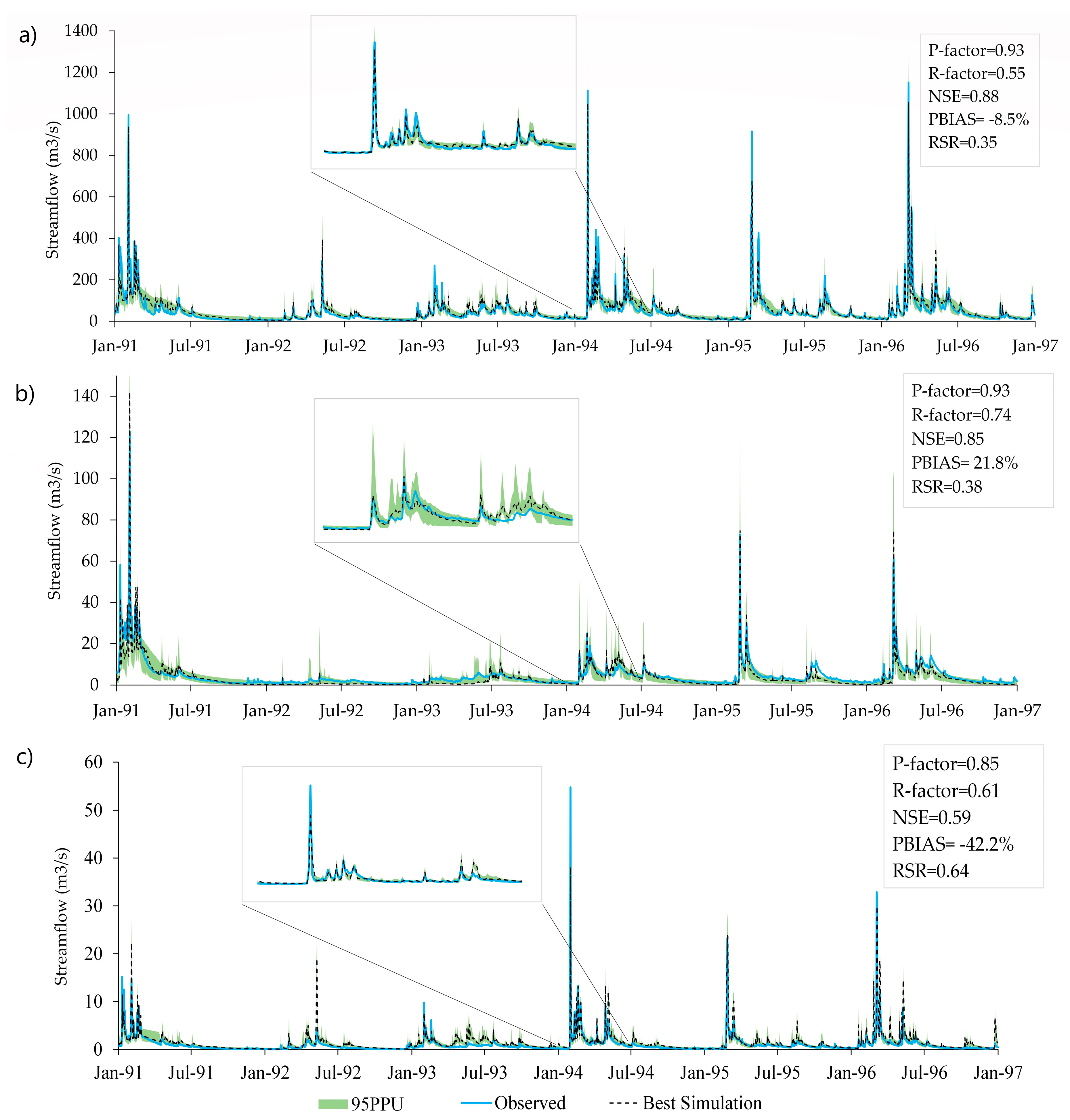
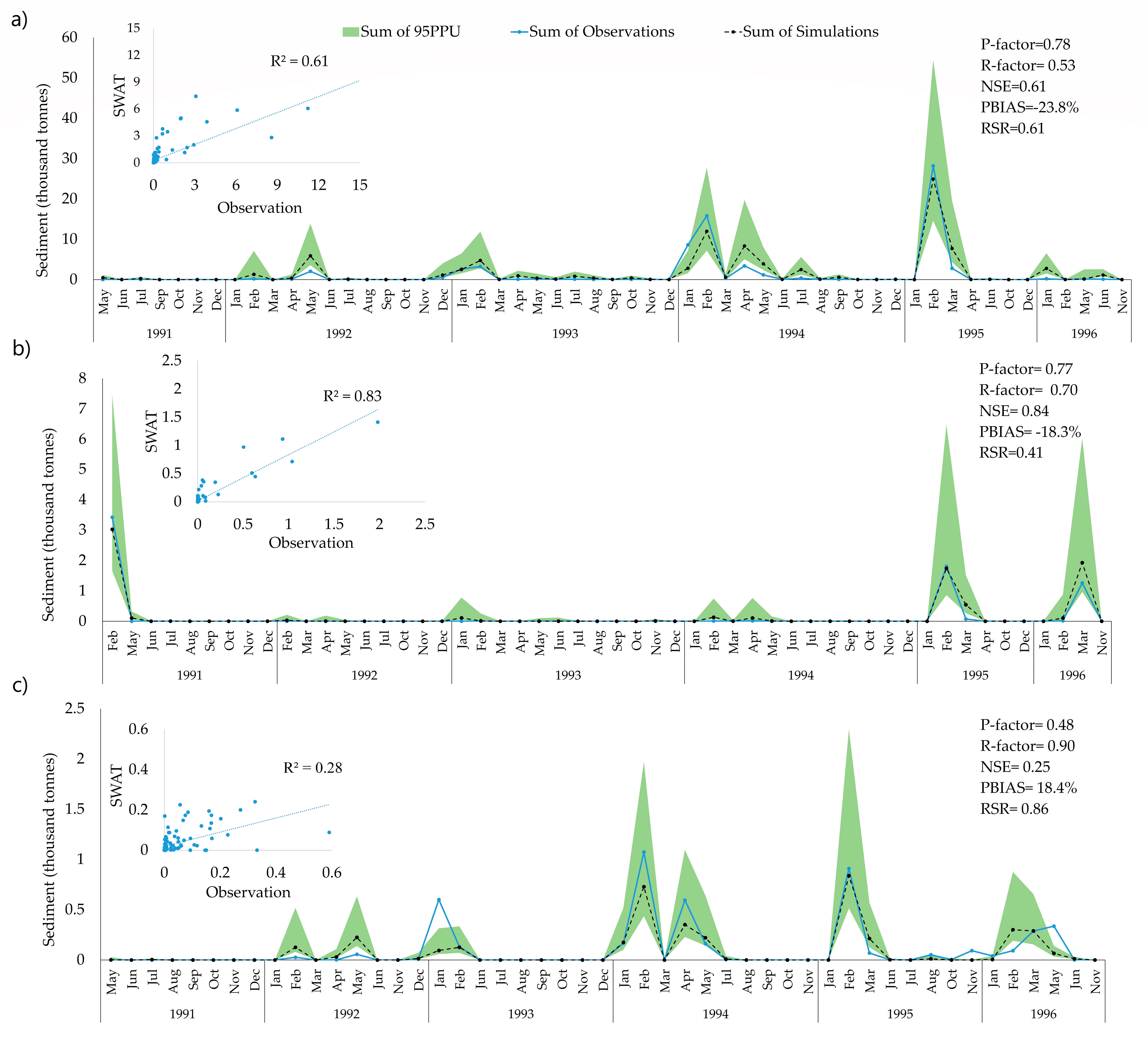
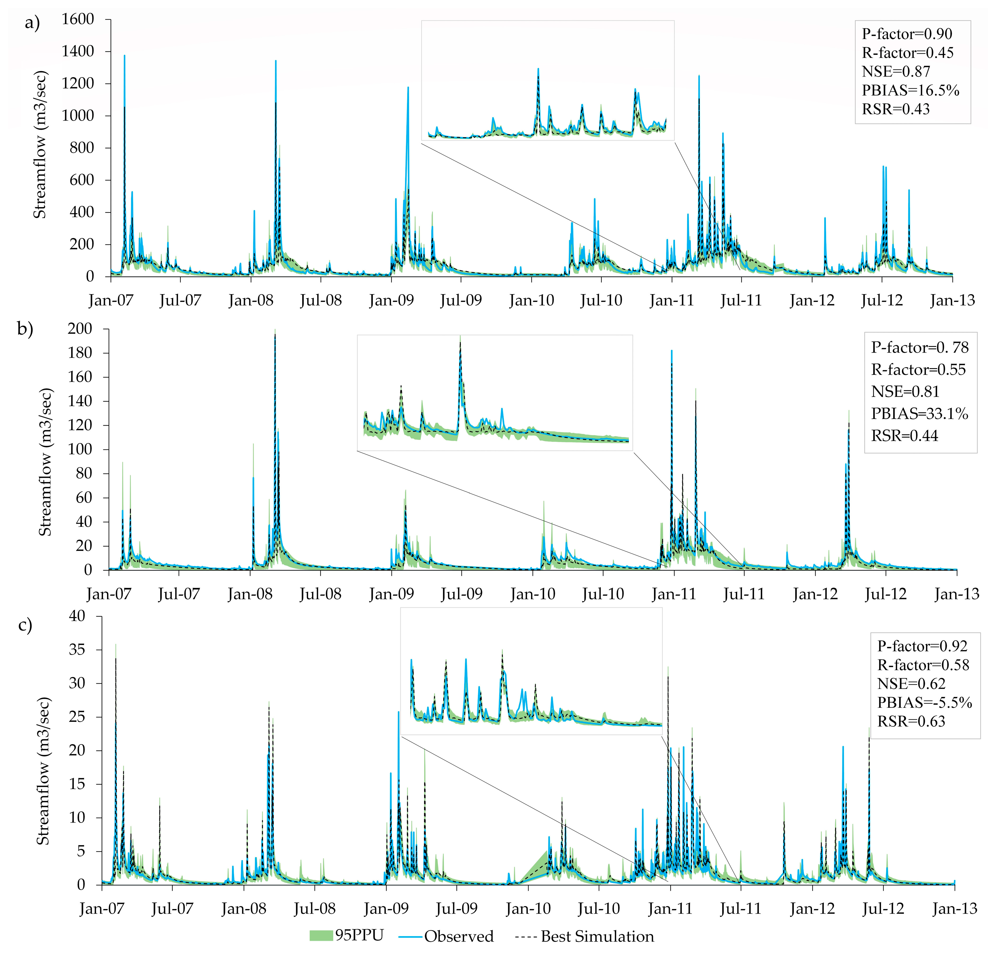
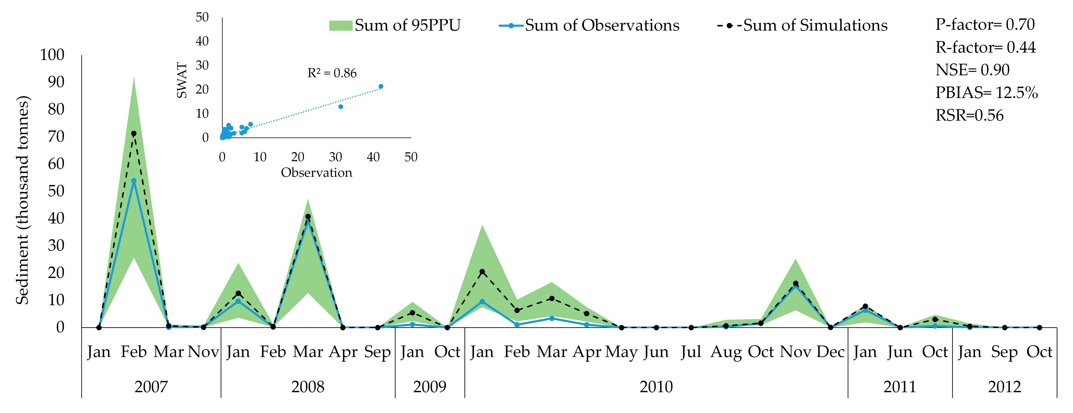
3.1. Model Calibration and Validation Results

Table 3 shows the global parameter sensitivity analysis for the calibration period (the smaller of p-value and larger absolute value of t-state determine the sensitivity ranking of the parameters). The parameters including USLE_C for pasture areas, USLE_K for the whole of the region, CH_N1 for all tributary channels in the region, USLE_C for farmlands (banana and sugarcane), CH_K1 for all tributary channels, CN2 and OV_N for pasture areas have the highest sensitivity. Generally, the parameters in the MUSLE have higher sensitivity because the observed data for sediment are fewer than those of streamflow. Additionally, pasture areas cover the highest proportion of the catchment, thus, although the soil erosion from farmlands is higher, much of the sediment loads is contributed by pasture areas, thus justifying the highest sensitivity of the model to USLE_C for pasture areas. The other parameters such as CN2, OV_N and CH_K1 also show high sensitivities since calculating peak flows (events that carry the highest amount of sediment) is highly dependent on the value of these parameters.
Figure 3 shows the results of calibration and uncertainty analyses of streamflow. Most of the observations at either catchment scale or sub-catchment scale are captured by the 95PPU (P-factor ranges from 0.85 to 0.93) with an acceptable band thickness (R-factor ranges from 0.55 to 0.74). Moreover, the model performance statistic measures (NSE, RSR and PBIAS) show a very good agreement between the best simulations and the observations. Also, the small extracted graphs in Figure 3 clearly show that the event peak flows and daily baseflow observations are well captured by SWAT simulations.
Figure 4 shows the results of sediment calibration and uncertainty quantification. More than 77% of all observed sediment loads are captured by the simulations at the Tung Oil station and the Glenn Allyn station with an acceptable band thickness (R-factor is 0.53 and 0.70, respectively). Reasonable agreements are also achieved between the best simulation and observation for these two stations as NSE values are more than 0.6, RSR values are less than 0.65 and absolute values for PBIAS are less than 25% (see Figure 4a,b). While the P-factor and NSE for Fisher Creek station is not desirable, the calibration performance for this station is still acceptable given the small drainage area of Fisher Creek station and the inherent errors in recording sediment concentrations and calculating sediment loads for such a sub-catchment with short lag time in the hydrograph. It should be noted that but most of the extreme sediment loads are captured by 95PPU (Figure 4c).
Figure 5 shows the results of the best streamflow simulation (using fitted values found from the best simulation in the calibration period) and uncertainty analysis (using the parameter range found from the calibration) for the validation period (2007–2012). Acceptable 95PPU was achieved for all gauging stations with P-factor ranging from 0.78 to 0.92 and R-factor ranging from 0.45 to 0.58. In addition, the best simulation predicted a reasonable estimation relative to observation for all gauging stations for the validation period (NSE between 0.62 and 0.87, RSR between 0.43 and 0.63 and PBIAS between −5 and 33%). The small extracted graphs in Figure 5 clearly show that the peak flows and daily base flow observations are well simulated by the model.
Similarly, as shown in Figure 6, good model predictive performance was achieved for sediment loads for the Tung Oil station—the only sediment monitoring station—as P-factor is 0.70 and R-factor is 0.44 while for the best simulation the NSE is 0.9, PBIAS is 12.5% and RSR is 0.56.

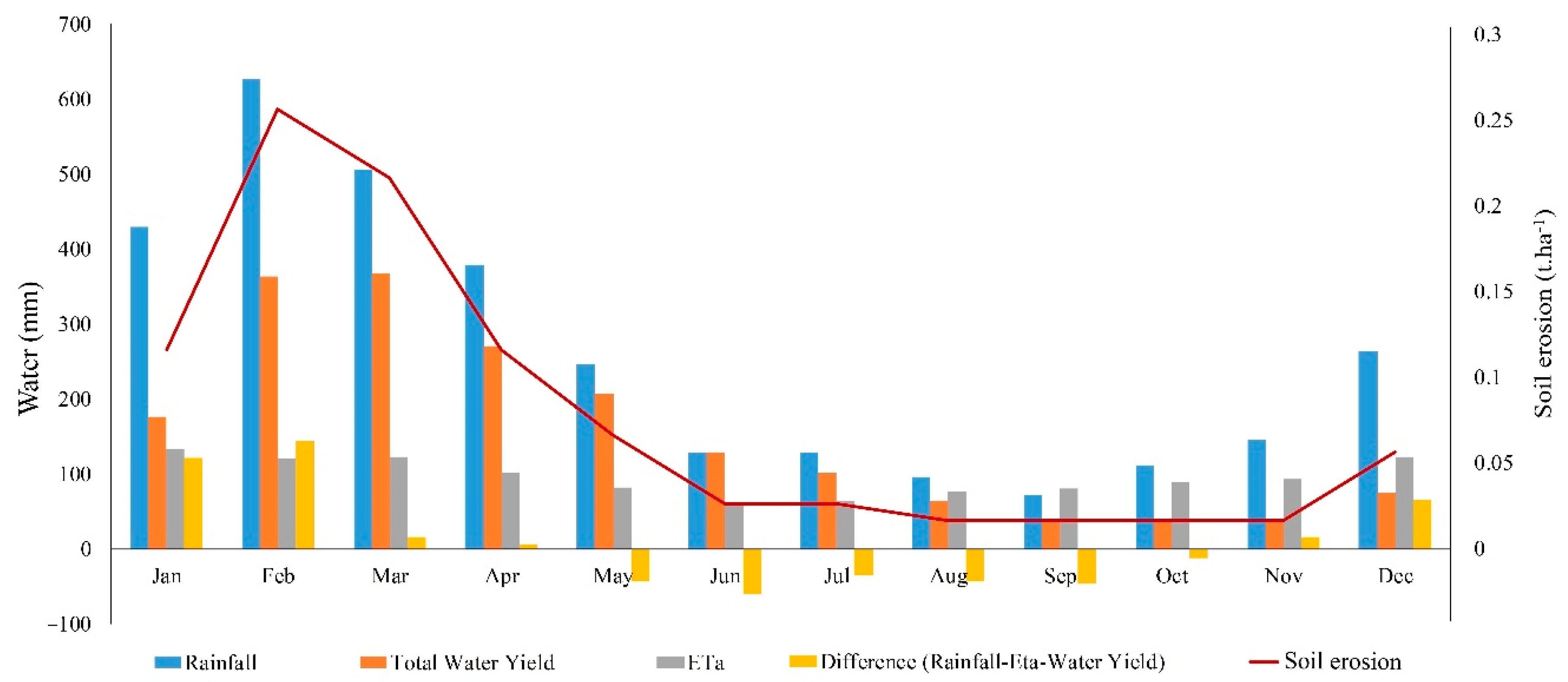
3.2. Water Balance and Sediment Budget

Table 4 shows the 95PPU and the annual average values for simulated water balance components over the 22 years of simulation. The results show that the average annual rainfall falling within the catchment is 3113 mm of which about 36% returns to the atmosphere through evapotranspiration. Predicted annual water yield is between 1860 and 2208 mm of which 977–1400 mm is surface runoff (around 31–44% of the whole rainfall), 248–292 mm is lateral flow, 469–855 mm and 35–48 mm are, respectively, return flows from shallow groundwater and deep aquifers and 12–313 mm leaves the system by transmission losses.
As illustrated in Figure 7, during summer months (November to April), the difference between rainfall and total amount of water leaving the catchment (water yield and ETa) is positive which indicates recharging groundwater and increasing stored water in soil. During the winter months (May to October), this value is negative, indicating a reduction in stored water in soil and the contribution of groundwater return flow to baseflow.
The simulated average annual soil erosion rate of the North Johnstone catchment ranges from 0.7 to 2.13 t∙ha–1. The average monthly water balance and soil erosion rate show a close correlation between water yield and soil erosion, with the highest soil erosion rate (0.25 t∙ha–1) in February, the month with the highest water yield and rainfall (Figure 7).
The spatial distribution of average annual surface runoff, groundwater return flow, ETa and rainfall in the North Johnstone catchment with respect to standard deviation are depicted in Figure 8. Our simulation results show that annual ETa in the upper section with high altitude is between 886 and 1077 mm and annual ETa in the midsection (rainforest dominated area) is between 1239 and 1489 mm. The results of the SWAT simulation show that rainforest dominated areas support the baseflow and a significant amount of groundwater return flow is generated from the rainforest areas in the middle section of the catchment while the upper section seldom contributes to baseflow.

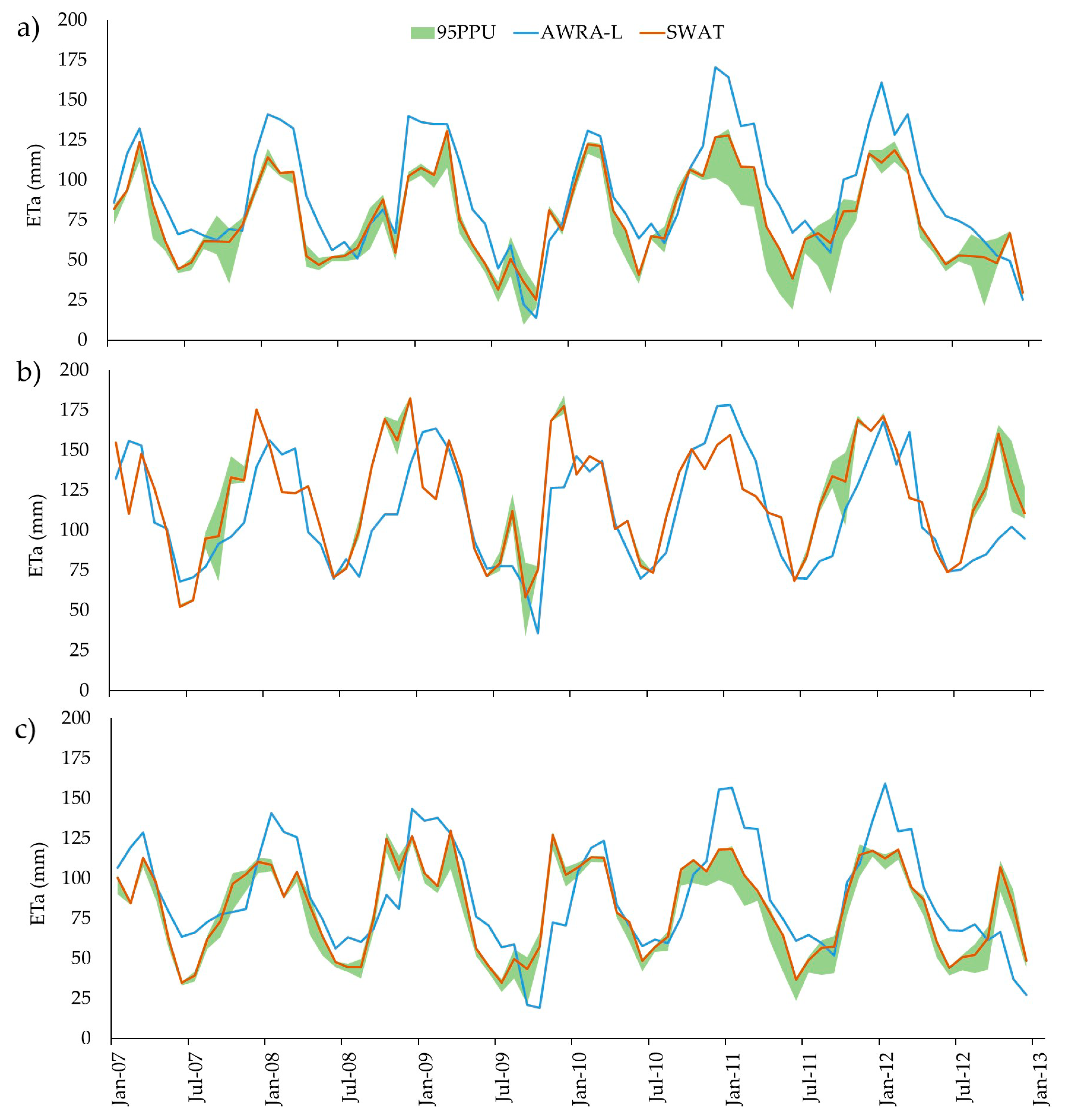
3.3. SWAT Performance in Simulating ETa Compared to AWRA-L
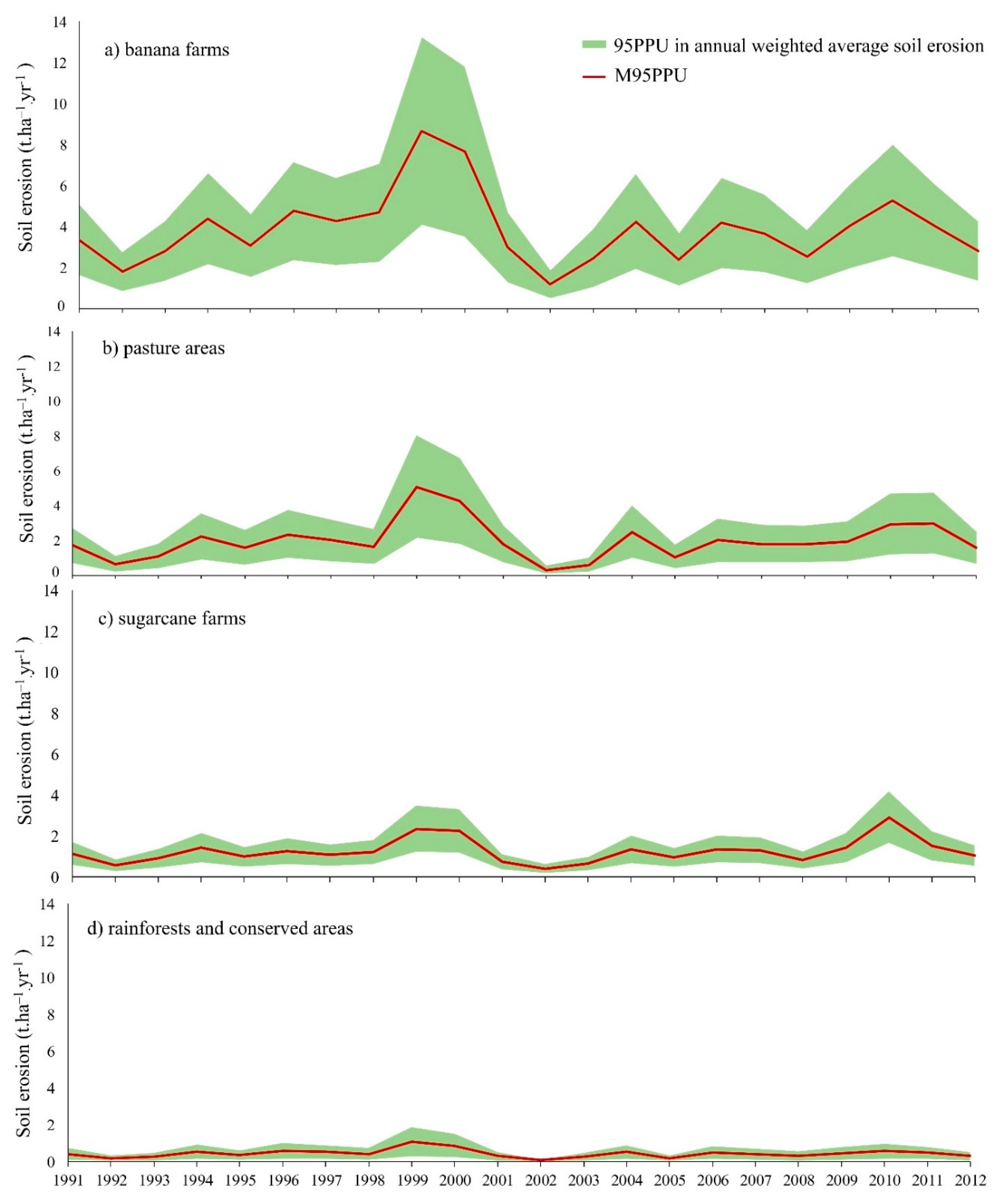
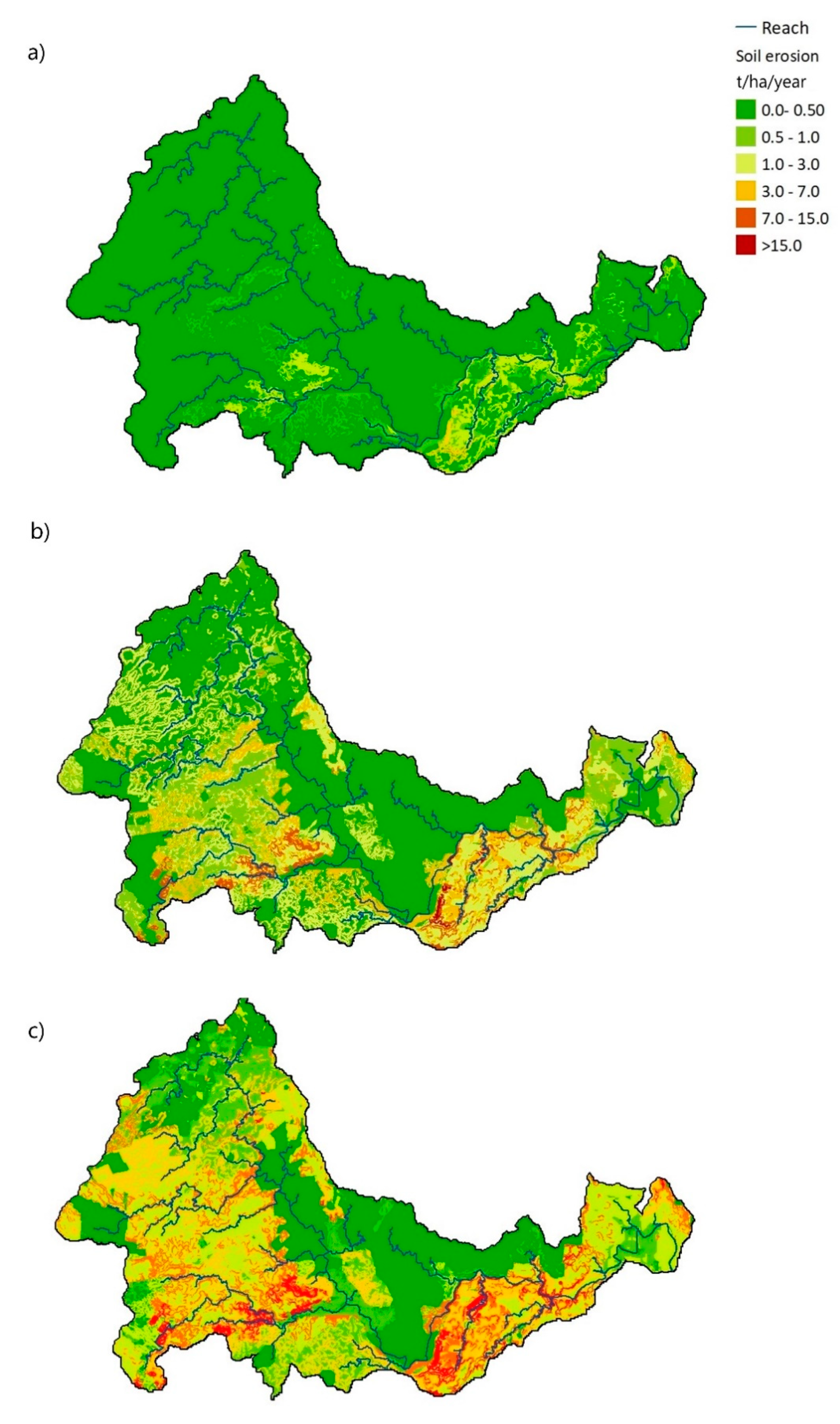
Average annual ETa simulated by SWAT for the pasture dominated area (Figure 9a) is between 794 mm and 961 mm, for the rainforest dominated location (Figure 9b) is between 1400 mm to 1485 mm and for the mixed pasture and rainforest location (Figure 9c) is between 872 mm and 1016 mm. For the same order, ETa by AWRA-L is estimated at 1089 mm, 1332 mm and 1071 mm. A direct comparison between SWAT and AWRA-L is not applicable as they are modelling ETa at different scales with different methods for estimating potential ET and water balance; however, the monthly ETa values simulated by SWAT are underestimated for location 1 and 3 (PBIAS values are respectively 16.1% and 8.0%), and overestimated for location 2 (with PBIAS of −8.3%) relative to monthly ETa values simulated by AWRA-L.

3.4. Soil Erosion

Figure 10 shows simulated annual time series of soil erosion with 95PPU for (a) banana HRUs (b) pasture HRUs (c) sugarcane HRUs and (d) rainforest HRUs over the 22 years of simulation (1991–2012). The 95PPU here represents the annual weighted average of soil erosion among the HRUs with the same land use based on their total land use area. Among the land uses, banana HRUs appear to have the highest annual soil erosion rate and associated predictive uncertainty, following by pasture HRUs and sugarcane HRUs. The rainforest HRUs appear to have lowest annual soil erosion as well as predictive uncertainty.
Table 5 shows the 95PPU of soil erosion rates among HRUs for the whole simulation period (1991–2012), classified based on slope range and land use. The median and mean of soil erosion rate are also included to show the tendency of simulated annual soil erosion rates. Accordingly, for a similar slope range, soil erosion rates in banana and sugarcane HRUs are about 1.5–2 times more than those of pasture HRUs and 10–12 times more than soil erosion in rainforests. For example, the 95PPU of soil erosion rates in pasture HRUs with less than 10% slope is between 0.03 and 2.73 t∙ha–1∙year−1 while the soil erosion for sugarcane and banana HRUs ranges from 0.19 to 5.63 t∙ha–1∙year−1 and 0.13 to 6.27 t∙ha–1∙year−1 respectively.
It should be noted that the highest proportion of pasture areas is located in the upper section where precipitation is half of the average of the catchment and surface runoff is relatively less than in the coastal zone where sugarcane and bananas are located (Figure 8b). The lower amount of rainfall/runoff plus the lower range of USLE_C values for the pasture HRUs are the main reasons behind less simulated soil erosion rate in pasture HRUs with the same slope range compared to sugarcane and bananas HRUs. However, when considering the annual weighted average of soil erosion rates among land uses (accounting for the effect of slope steepness), the annual weighted average of simulated soil erosion in banana and pasture HRUs is higher than in sugarcane HRUs, as 12% of banana HRUs and 39% of pasture HRUs are located on slope ranges of more than 10%, while this value is only 3% for sugarcane HRUs. The highest soil erosion for all land uses occurred in 1999—the most extreme wet year—that the mean of the annual weighted average (M95PPU) for bananas HRUs was 8.2 t∙ha–1∙year−1, for pasture HRUs was 4.65 t∙ha–1∙year−1, for sugarcane HRUs was 2.12 t∙ha–1∙year−1 and for rainforest HRUs was 0.96 t∙ha–1∙year−1. Moreover, the lowest soil erosion occurred in 2002 where the values of M95PPU for all land uses are less than 1 t∙ha–1∙year−1.
Figure 11 depicts the spatial maps of soil erosion under the extreme dry year (2002), the average of the simulation period (1991–2012) (Figure 11b), and the extreme wet year (1999) (Figure 11c). Average annual soil erosion rate for the catchment in the extreme dry year is 0.44 t∙ha–1∙year−1, while the average for the simulation period is 1.88 t∙ha–1∙year−1 and for the extreme wet year is 4.32 t∙ha–1∙year−1. The standard deviation of soil erosion rates for all land uses for the extreme dry year is 0.96, for the average of simulation period is 3.20 and for the extreme wet year is 7.34. The 97.5 percentile of soil erosion among all land uses for the extreme dry year is 0.96, for average of the simulation period is 9.88 t∙ha–1∙year−1 and for the extreme wet year is 20.75 t∙ha–1∙year−1. The coastal zone and the upper section of the catchment, dominated by sugarcane, bananas and pasture HRUs, are sensitive to rainfall, while the middle section of the catchment, dominated by rainforests, seldom changes with fluctuations in rainfall as they generate relatively low surface runoff as shown in Figure 8b.

4. Discussion

4.1. Comparison Soil Erosion with Previous Studies

In previous modelling efforts, the sediment and soil erosion for this catchment has been estimated, however, we designed this research to further investigate the details of water balance components, the impact of slope steepness and spatio-temporal variations on soil erosion across the North Johnstone catchment. The SWAT simulated streamflow rate, ETa and sediment loads were in reasonable agreement with observed values and the predictive uncertainty of model simulations could capture most of the observation with an acceptable error band thickness. This indicates that the model provided a good representation of catchment hydrology and soil erosion.
Our modelling results were also in agreement with Hunter and Walton [13] that used the Hydrological Simulation Program—FORTRAN (HSPF) model to simulate constituent loads including sediment fluxes from North and South Johnstone to GBR. The authors estimated sediment fluxes from banana (4.0 ± 2.5 t∙ha–1∙year−1), sugarcane (3.8 ± 2.5 t∙ha–1∙year−1), rainforests and pasture areas (1.2 ± 1.1 t∙ha–1∙year−1). However, although we found a similar level of soil erosion in banana and sugarcane farms within the same slope range (Table 5), when taking into account the effect of slope steepness, we found that annual weighted average of soil erosion among banana and pasture HRUs is higher than in sugarcane HRUs as only 3% of sugarcane areas have slope range more than 10%, while this value is 12% for banana land use and 39% for pasture land use.

4.2. Hillslope Soil Erosion Modelling for GBR Catchments

The RUSLE model which is a derivative version of the USLE model with some improvement in erosion controlling factors has been widely used for estimating hillslope soil erosion for Australian catchments. However, continuous research showed that RUSLE generally overestimates soil erosion, especially for steep rainforest areas [14,57]. To resolve this overestimation, in current modelling sediment loads for GBR by the Reef Water Quality Protection Plan, the RUSLE model is only being applied for grazing land use and the Event Mean Concentration/Dry Weather Concentration (EMC/DWC) model being used for modelling erosion in rainforests and banana farms [17]. However, EMC/DWC cannot account for hillslope erosion and further improvement is required [17]. A clear example for overestimation of RUSLE is Teng et al. [58] who used the RUSLE to estimate soil erosion for the Australian continent. Teng et al. [58] reported that based on their modelling results, the Johnstone catchment has large rates of soil erosion and predicted more than 50 t∙ha–1∙year−1 soil erosion for the rainforest dominated area in the middle section of the catchment. In a notable contrast, the SWAT model which uses the MUSLE model and replaces the rainfall erosivity factor in RUSLE by the runoff factor, predicted more accurately a significantly lower amount of soil erosion for the rainforest dominated area. Furthermore, our soil erosion results for banana land use can be directly compared with a recent paddock scale sediment monitoring in the Johnstone catchment [59] which showed during the water year of 2010–2011 that the farm received more than 5000 mm rainfall, and the soil erosion (the farm had no management practices such grassed inter row) was around 11 t∙ha–1∙year−1. Our modelling results also show that in an extreme wet year with more than 5000 mm rainfall, the weighted average of soil erosion for banana HRUs can be as low as 3 t∙ha–1∙year−1 and as high as 13 t∙ha–1∙year−1. However, although using MUSLE could more accurately predict soil erosion, this approach required a sophisticated and computationally extensive calibration and validation for both hydrology and sediment load.

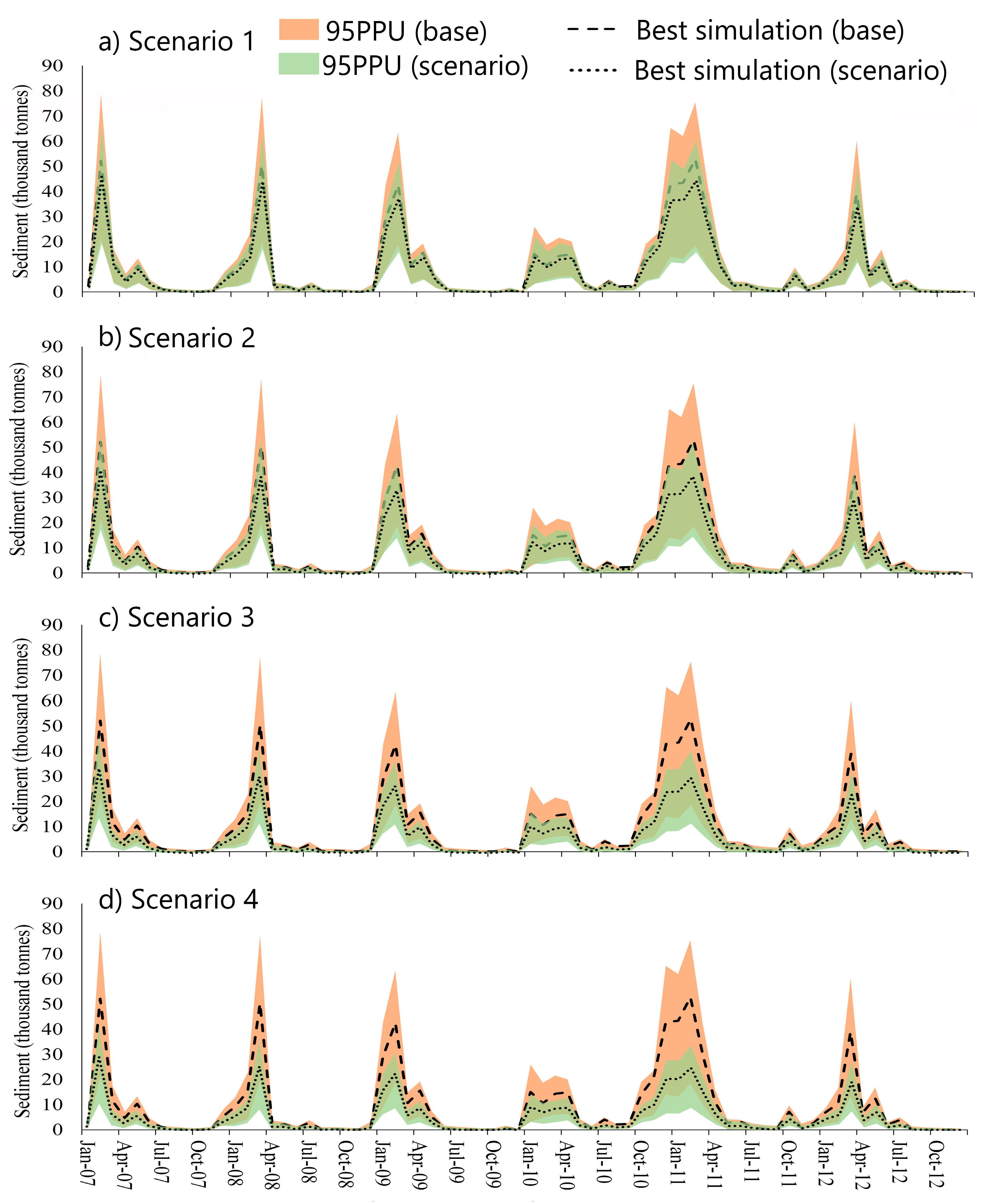
4.3. The Effectiveness of Reforestation on Steep Slopes

The hypothesis that reforestation can reduce sediment is examined here by using a set of scenarios and with the assistance of the SWAT model validated for this region. For this purpose, we designed four land-use change scenarios from pasture to rainforests based on four slope groups for a six-year period (Figure 12). As reforestation is not an instantaneous process, we considered that reforestation in designated pasture areas initiated in 1991 and restored forests reached full maturity in 2007. Hence, for the first scenario, we converted all pasture land uses with more than 30% slope (4071 ha) to rainforests. The results show that changing land use in these steep slope areas to rainforests reduced 15% sediment loads within six years which is equal to 25,000 tonnes per year. In the second scenario, pasture areas with more than 20% slope (9342 ha) are converted into rainforest which resulted in 26% reduction in sediment delivery to GBR (equal to 45,000 tonnes per year). In the third scenario, all pasture areas with more than 10% slope (21,724 ha) are converted into rainforests and resulted in a 40% reduction in sediment loads at the end of the catchment. Finally, converting all pasture areas to rainforest (55,487 ha) showed just a subtle difference from the third scenario (47% reduction in total sediment loads).
Overall, based on these modelling results, further management practices (e.g., reforestation and grassed inter row) for reducing soil erosion should be prioritised in high slope areas, specifically in pasture areas and banana farms. The identified sediment hotspots in this study can be considered for implanting further monitoring stations or used for carrying out soil erosion studies. Moreover, to reduce predictive uncertainty for simulating soil erosion from banana farms in the future modelling, a database that shows the spatial map of management practices can significantly improve the output.

5. Conclusions

In this research, we assessed hydrological processes and soil erosion and identified hotspots for management interventions in a tropical catchment of GBR. The SWAT model was applied to the North Johnstone catchment. The parameterisation of biophysical processes such as plant growth and ground cover were carried out using remote sensing database or field based studies. We calibrated and validated the model and quantified predictive uncertainty in simulating streamflow and sediment loads at the catchment and sub-catchment scale. The results were in reasonable agreement to observed values. For further analysis, the impact of slope steepness and spatio-temporal variations on soil erosion across the catchment were rigorously investigated. Finally, four land use change scenarios were applied to evaluate the effectiveness of converting pasture areas to rainforests in reducing sediment fluxes to GBR. Our results show that converting pasture areas with slopes more than 30% and 20% which cover 4% and 9% of the catchment, can potentially reduce 15% and 26% of the annual sediment loads to GBR.

Author Contributions

Conceptualization, V.R. and A.G.; methodology, V.R. and A.G.; software, V.R.; validation, V.R., A.G. and D.-A.A.-V.; formal analysis, V.R.; investigation, V.R.; resources, S.M. and D.-A.A.-V.; data curation, V.R. and A.G.; writing—original draft preparation, V.R.; writing—review and editing, D.-A.A.-V., A.G. and S.M.; visualization, V.R.; supervision, S.M., A.G. and D.-A.A.-V.; project administration, S.M. All authors have read and agreed to the published version of the manuscript.

Funding

This research received no external funding.

Acknowledgments

We acknowledge the University of Southern Queensland for providing an international fees research scholarship to the first author. We thank the State of Queensland (Department of Environment and Science) for providing monitoring data. The authors also acknowledge the helpful proofreading work from Barbara Harmes and reviewers for providing valuable comments, which improved this manuscript.

Conflicts of Interest

The authors declare no conflicts of interest.

References

  1. Griggs, P.D. Too much water: Drainage schemes and landscape change in the sugar-producing areas of Queensland, 1920–1990. Aust. Geogr. 2018, 49, 81–105. [Google Scholar] [CrossRef]
  2. Evans, M.C. Deforestation in Australia: Drivers, trends and policy responses. Pac. Conserv. Biol. 2016, 22, 130–150. [Google Scholar] [CrossRef]
  3. Rasiah, V.; Florentine, S.K.; Williams, B.L.; Westbrooke, M.E. The impact of deforestation and pasture abandonment on soil properties in the wet tropics of Australia. Geoderma 2004, 120, 35–45. [Google Scholar] [CrossRef] [Green Version]
  4. Bradshaw, C.J. Little left to lose: Deforestation and forest degradation in Australia since European colonization. Plant Ecol. 2012, 5, 109–120. [Google Scholar] [CrossRef]
  5. Kroon, F.J. Towards ecologically relevant targets for river pollutant loads to the Great Barrier Reef. Mar. Pollut. Bull. 2012, 65, 261–266. [Google Scholar] [CrossRef]
  6. Waterhouse, J.; Brodie, J.; Tracey, D.; Smith, R.; Vandergragt, M.; Collier, C.; Petus, C.; Baird, M.; Kroon, F.; Mann, R.; et al. The Risk from Anthropogenic Pollutants to Great Barrier Reef Coastal and Marine Ecosystems. In Scientific Consensus Statement 2017: A Synthesis of the Science of Land-Based Water Quality Impacts on the Great Barrier Reef; Queensland Department of Environment and Science: Brisbane, Australia, 2017. Available online: https://www.reefplan.qld.gov.au/__data/assets/pdf_file/0032/45995/2017-scientific-consensus-statement-summary-chap03.pdf (accessed on 1 August 2020).
  7. Waterhouse, J.; Schaffelke, B.; Bartley, R.; Eberhard, R.; Brodie, J.; Star, M.; Thorburn, P.; Rolfe, J.; Ronan, M.; Taylor, B.; et al. Overview of Key Findings, Management Implications and Knowledge Gaps. In 2017 Scientific Consensus Statement: Land Use Impacts on the Great Barrier Reef Water Quality and Ecosystem Condition; Queensland Department of Environment and Science: Brisbane, Australia, 2017. Available online: https://www.reefplan.qld.gov.au/__data/assets/pdf_file/0034/45997/2017-scientific-consensus-statement-summary-chap05.pdf (accessed on 1 August 2020).
  8. Bartley, R.; Thompson, C.; Croke, J.; Pietsch, T.; Baker, B.; Hughes, K.; Kinsey-Henderson, A. Insights into the history and timing of post-European land use disturbance on sedimentation rates in catchments draining to the Great Barrier Reef. Mar. Pollut. Bull. 2018, 131, 530–546. [Google Scholar] [CrossRef] [PubMed]
  9. Hairsine, P.B. Sediment-Related Controls on the Health of the Great Barrier Reef. Vadose Zone J. 2017, 16, 1–15. [Google Scholar] [CrossRef] [Green Version]
  10. Ebner, B.C.; Fulton, C.J.; Donaldson, J.A.; Schaffer, J. Distinct habitat selection by freshwater morays in tropical rainforest streams. Ecol. Freshw. Fish. 2016, 25, 329–335. [Google Scholar] [CrossRef]
  11. Wilkinson, S.N.; Dougall, C.; Kinsey-Henderson, A.E.; Searle, R.D.; Ellis, R.J.; Bartley, R. Development of a time-stepping sediment budget model for assessing land use impacts in large river basins. Sci. Total Environ. 2014, 468, 1210–1224. [Google Scholar] [CrossRef] [PubMed] [Green Version]
  12. Herr, A.; Kuhnert, P.M. Assessment of uncertainty in Great Barrier Reef catchment models. Water Sci. Technol. 2007, 56, 181–188. [Google Scholar] [CrossRef] [PubMed]
  13. Hunter, H.M.; Walton, R.S. Land-use effects on fluxes of suspended sediment, nitrogen and phosphorus from a river catchment of the Great Barrier Reef, Australia. J. Hydrol. 2008, 356, 131–146. [Google Scholar] [CrossRef]
  14. Armour, J.D.; Hateley, L.R.; Pitt, G.L. Catchment modelling of sediment, nitrogen and phosphorus nutrient loads with SedNet/ANNEX in the Tully–Murray basin. Mar. Freshw. Res. 2009, 60, 1091–1096. [Google Scholar] [CrossRef] [Green Version]
  15. Gladish, D.W.; Kuhnert, P.M.; Pagendam, D.E.; Wikle, C.K.; Bartley, R.; Searle, R.D.; Ellis, R.J.; Dougall, C.; Turner, R.D.; Lewis, S.E.; et al. Spatio-temporal assimilation of modelled catchment loads with monitoring data in the Great Barrier Reef. Ann. Appl. Stat. 2016, 10, 1590–1618. [Google Scholar] [CrossRef]
  16. Hughes, A.O.; Croke, J.C. Validation of a spatially distributed erosion and sediment yield model (SedNet) with empirically derived data from a catchment adjacent to the Great Barrier Reef Lagoon. Mar. Freshw. Res. 2011, 62, 962–973. [Google Scholar] [CrossRef]
  17. Hateley, L.R.; Ellis, R.; Shaw, M.; Waters, D.; Carroll, C. Modelling Reductions of Pollutant Loads Due to Improved Management Practices in the Great Barrier Reef Catchments—Wet Tropics NRM Region; Technical Report; Queensland Department of Natural Resources and Mines: Cairns, Australia, 2014; Volume 3, ISBN 978-0-7345-0441-8.
  18. An-Vo, D.A.; Mushtaq, S.; Reardon-Smith, K.; Kouadio, L.; Attard, S.; Cobon, D.; Stone, R. Value of seasonal forecasting for sugarcane farm irrigation planning. Eur. J. Agron. 2019, 104, 37–48. [Google Scholar] [CrossRef]
  19. An-Vo, D.A.; Reardon-Smith, K.; Mushtaq, S.; Cobon, D.; Kodur, S.; Stone, R. Value of seasonal climate forecasts in reducing economic losses for grazing enterprises: Charters Towers case study. Rangel. J. 2019, 41, 165–175. [Google Scholar] [CrossRef] [Green Version]
  20. Henderson, B.; Bui, E. Determining Uncertainty in Sediment & Nutrient Transport Models for Ecological Risk Assessment (No. 2); CSIRO: Canberra, Australia, 2005. [Google Scholar]
  21. Fu, B.; Merritt, W.S.; Croke, B.F.; Weber, T.; Jakeman, A.J. A review of catchment-scale water quality and erosion models and a synthesis of future prospects. Environ. Model. Softw. 2019, 114, 75–97. [Google Scholar] [CrossRef]
  22. Neitsch, S.L.; Arnold, J.G.; Kiniry, J.R.; Williams, J.R. Soil and Water Assessment Tool Theoretical Documentation Version 2009; Texas Water Resources Institute: College Station, TX, USA, 2011. [Google Scholar]
  23. Abbaspour, K.C. SWAT-CUP4: SWAT Calibration and Uncertainty Programs—A User Manual; Swiss Federal Institute of Aquatic Science and Technology, Eawag: Überland, Switzerland, 2011. [Google Scholar]
  24. Bartley, R.; Waters, D.; Turner, R.; Kroon, F.; Wilkinson, S.; Garzon-Garcia, A.; Kuhnert, P.; Lewis, S.; Smith, R.; Bainbridge, Z.; et al. Sources of Sediment, Nutrients, Pesticides and other Pollutants to the Great Barrier Reef. In Scientific Consensus Statement 2017: A Synthesis of the Science of Land-Based Water Quality Impacts on the Great Barrier Reef; Queensland Department of Environment and Science: Brisbane, Australia, 2017. Available online: https://www.reefplan.qld.gov.au/__data/assets/pdf_file/0031/45994/2017-scientific-consensus-statement-summary-chap02.pdf (accessed on 1 August 2020).
  25. Wilkinson, C.; Brodie, J. Catchment Management and Coral Reef Conservation; James Cock University: Douglas, Australia, 2011. [Google Scholar]
  26. Marden, M. Effectiveness of reforestation in erosion mitigation and implications for future sediment yields, East Coast catchments, New Zealand: A review. N. Z. Geog. 2012, 68, 24–35. [Google Scholar] [CrossRef]
  27. Delevaux, J.M.; Whittier, R.; Stamoulis, K.A.; Bremer, L.L.; Jupiter, S.; Friedlander, A.M.; Poti, M.; Guannel, G.; Kurashima, N.; Winter, K.B.; et al. A linked land-sea modeling framework to inform ridge-to-reef management in high oceanic islands. PLoS ONE 2018, 13, e0193230. [Google Scholar] [CrossRef] [Green Version]
  28. Faruqi, S.; Wu, A.; Brolis, E.; Ortega, A.A.; Batista, A. The Business of Planting Trees: A Growing Investment Opportunity; World Resources Institute: Washington, DC, USA, 2018. [Google Scholar]
  29. Carlson, R.R.; Foo, S.A.; Asner, G.P. Land use impacts on coral reef health: A ridge-to-reef perspective. Front. Mar. Sci. 2019, 6, 562. [Google Scholar] [CrossRef]
  30. Preece, N.D.; Van Oosterzee, P.; Lawes, M.J. Planting methods matter for cost-effective rainforest restoration. Ecol. Manag. Restor. 2013, 14, 63–66. [Google Scholar] [CrossRef]
  31. Cheesman, A.W.; Preece, N.D.; van Oosterzee, P.; Erskine, P.D.; Cernusak, L.A. The role of topography and plant functional traits in determining tropical reforestation success. J. Appl. Ecol. 2018, 55, 1029–1039. [Google Scholar] [CrossRef] [Green Version]
  32. Ndomba, P.; Mtalo, F.; Killingtveit, A. SWAT model application in a data scarce tropical complex catchment in Tanzania. Phys. Chem. Earth 2008, 33, 626–632. [Google Scholar] [CrossRef]
  33. Alansi, A.W.; Amin, M.S.M.; Halim, F.A.; Shafri, H.Z.M.; Aimrum, W. Validation of SWAT model for stream flow simulation and forecasting in Upper Bernam humid tropical river basin, Malaysia. Hydrol. Earth. Syst. Sci. Discuss. 2009, 1, 6. [Google Scholar] [CrossRef]
  34. Fukunaga, D.C.; Cecílio, R.A.; Zanetti, S.S.; Oliveira, L.T.; Caiado, M.A.C. Application of the SWAT hydrologic model to a tropical watershed at Brazil. Catena 2015, 125, 206–213. [Google Scholar] [CrossRef]
  35. Williams, J.R.; LaSeur, W.V. Water yield model using SCS curve numbers. J. Hydr. Eng. DIV 1976, 102, 12379. [Google Scholar]
  36. Monteith, J.L. Evaporation and environment. In Symposia of the Society for Experimental Biology; Cambridge University Press: Cambridge, UK, 1965; pp. 205–234. [Google Scholar]
  37. Hargreaves, G.L.; Hargreaves, G.H.; Riley, J.P. Irrigation water requirements for Senegal River basin. J. Irrig. Drain. E-ASCE 1985, 111, 265–275. [Google Scholar] [CrossRef]
  38. Priestley, C.H.B.; Taylor, R.J. On the assessment of surface heat flux and evaporation using large-scale parameters. Mon. Weather Rev. 1972, 100, 81–92. [Google Scholar] [CrossRef]
  39. Willams, J.R. Sediment-yield prediction with universal equation using runoff energy factor. In Present and Prospective Technology for Predicting Sediment Yields and Sources; US Department of Agriculture, Agriculture Research Service: Washington, DC, USA, 1975. [Google Scholar]
  40. Williams, J.R.; Berndt, H.D. Sediment yield prediction based on watershed hydrology. Trans. ASAE 1977, 20, 1100–1104. [Google Scholar] [CrossRef]
  41. Bagnold, R.A. Bed load transport by natural rivers. Water Resour. Res. 1977, 13, 303–312. [Google Scholar] [CrossRef]
  42. Bureau of Agricultural and Resource Economics and Sciences. The Australian Land Use and Management Classification Version 8; Bureau of Agricultural and Resource Economics and Sciences: Canberra, Australia, 2016.
  43. McKenzie, N.J.; Jacquier, D.W.; Maschmedt, D.J.; Griffin, E.A.; Brough, D.M. The Australian Soil Resource Information System (ASRIS) Technical Specifications, Revised Version 1.6; CSIRO: Canberra, Australia, 2012.
  44. Walling, D.E.; WEBB, B.W. The Reliability of Suspended Sediment Load Data. In Erosion and Sediment Transport Measurement, Proceedings of the Florence Symposium, Firenze, Italy, 22–26 June 1981; Volume 133, pp. 177–194. Available online: https://iahs.info/uploads/dms/iahs_133_0177.pdf (accessed on 1 August 2020).
  45. Frost, A.J.; Ramchurn, A.; Smith, A. The Australian Landscape Water Balance Model. (AWRA-L v6). Technical Description of the Australian Water Resources Assessment Landscape Model. Version 6; Bureau of Meteorology Technical Report: Melbourne, Australia, 2018.
  46. Daggupati, P.; Pai, N.; Ale, S.; Douglas-Mankin, K.R.; Zeckoski, R.W.; Jeong, J.; Parajuli, P.B.; Saraswat, D.; Youssef, M.A. A recommended calibration and validation strategy for hydrologic and water quality models. Trans. ASABE 2015, 58, 1705–1719. [Google Scholar]
  47. Baez-Gonzalez, A.D.; Kiniry, J.R.; Meki, M.N.; Williams, J.; Alvarez-Cilva, M.; Ramos-Gonzalez, J.L.; Magallanes-Estala, A.; Zapata-Buenfil, G. Crop parameters for modeling sugarcane under rainfed conditions in Mexico. Sustainability 2017, 9, 1337. [Google Scholar] [CrossRef] [Green Version]
  48. Robertson, M.J.; Bonnett, G.D.; Hughes, R.M.; Muchow, R.C.; Campbell, J.A. Temperature and leaf area expansion of sugarcane: Integration of controlled-environment, field and model studies. Funct. Plant. Biol. 1998, 25, 819–828. [Google Scholar] [CrossRef]
  49. Keating, B.A.; Robertson, M.J.; Muchow, R.C.; Huth, N.I. Modelling sugarcane production systems I. Development and performance of the sugarcane module. Field Crops. Res. 1999, 61, 253–271. [Google Scholar] [CrossRef]
  50. Guimarães, M.J.M.; Coelho Filho, M.A.; Peixoto, C.P.; Gomes Junior, F.D.A.G.; Oliveira, V.V.M. Estimation of leaf area index of banana orchards using the method LAI-LUX. Water Resour. Irrig. Manag. 2013, 2, 71–76. [Google Scholar]
  51. Gilmour, D.A. Catchment Water Balance Studies on the Wet Tropical Coast of North Queensland. Ph.D. Thesis, James Cook University, Townsville, Australia, 1975. [Google Scholar]
  52. Moriasi, D.N.; Zeckoski, R.W.; Arnold, J.G.; Baffaut, C.; Malone, R.W.; Daggupati, P.; Guzman, J.A.; Saraswat, D.; Yuan, Y.; Wilson, B.N.; et al. Hydrologic and water quality models: Key calibration and validation topics. Trans. ASABE 2015, 58, 1609–1618. [Google Scholar]
  53. Abbaspour, K.C.; Johnson, C.A.; Van Genuchten, M.T. Estimating uncertain flow and transport parameters using a sequential uncertainty fitting procedure. Vadose Zone J. 2004, 3, 1340–1352. [Google Scholar] [CrossRef]
  54. McKay, M.D.; Beckman, R.J.; Conover, W.J. Comparison of three methods for selecting values of input variables in the analysis of output from a computer code. Technometrics 1979, 21, 239–245. [Google Scholar]
  55. Abbaspour, K.C.; Vaghefi, S.A.; Srinivasan, R. A guideline for successful calibration and uncertainty analysis for soil and water assessment: A review of papers from the 2016 International SWAT Conference. Water 2018, 10, 6. [Google Scholar] [CrossRef] [Green Version]
  56. Arnold, J.G.; Allen, P.M. Automated methods for estimating baseflow and ground water recharge from streamflow records 1. J. Am. Water. Resour. Assoc. 1999, 35, 411–424. [Google Scholar] [CrossRef]
  57. Brooks, A.; Spencer, J.; Borombovits, D.; Pietsch, T.; Olley, J. Measured hillslope erosion rates in the wet-dry tropics of Cape York, northern Australia: Part 2, RUSLE-based modeling significantly over-predicts hillslope sediment production. Catena 2014, 122, 1–17. [Google Scholar] [CrossRef]
  58. Teng, H.; Rossel, R.A.V.; Shi, Z.; Behrens, T.; Chappell, A.; Bui, E. Assimilating satellite imagery and visible–near infrared spectroscopy to model and map soil loss by water erosion in Australia. Environ. Model. Softw. 2016, 77, 156–167. [Google Scholar] [CrossRef]
  59. Armour, J.D.; Davis, A.; Masters, B.; Mortimore, C.; Whitten, M. Paddock Scale Water Quality Monitoring of Sugarcane and Banana Management Practices: Final Technical Report 2010–2013 Wet Seasons; Wet Tropics Region, Queensland Department of Natural Resources and Mines, Centre for Tropical Water & Aquatic Ecosystem Research and Queensland Department of Agriculture, Fisheries and Forestry for Terrain Natural Resource Management: Mareeba, Australia, 2013. [Google Scholar]
Figure 1. The location of the North Johnstone catchment and its adjacent catchments in the Wet Tropics Region (a) and the upscaled North Johnstone catchment showing its river network and elevation gradient (b).
Water 12 02179 g001
Figure 2. (a) land use map, (b) soil layer map, (c) slope classification and (d) catchment details including the location of weather stations, monitoring stations, catchment outlet, river and streams. Legends of the soil layers represent their soil feature names and associated feature ID numbers in the ASRIS database in which the Gh1 is red smooth-ped earths moderately undulating lands; KHB is Krasnozems of the undulating and rolling hills on; KLB is Krasnozems of the basalt lava plains; KUB is Krasnozems of the undulating basalt lava plains; LN1 is pale loams with a smooth-ped B horizon; LN2 is pale loams with a smooth-ped B horizon, high hills; Mf19 is yellow smooth-ped earths, strongly undulating; Mj8 is red smooth-ped earths, hilly high plateau; Mp18 is red smooth-ped earths, moderately undulating lands; Mp19 is red smooth-ped earths, low hilly to hilly basalt; RMV is red podzolics of the steep hills and mountains.
Water 12 02179 g002
Figure 3. Streamflow calibration and uncertainty analysis: (a) Tung Oil station near the outlet of the catchment, (b) Glenn Allyn station in the upper section, and (c) Fisher Creek station.
Water 12 02179 g003
Figure 4. Results of calibration for sediment loads, showing aggregated values for each month in the calibration period of the best simulation, 95PPU, and the observation. The scatter plots show the best simulation versus the observation while the main graphs represent the monthly aggregated sediment loads: (a) Tung Oil station, (b) Glenn Allyn station, and (c) Fisher Creek station.
Water 12 02179 g004
Figure 5. Daily streamflow validation (the period between 2007 and 2012) and 95PPU: (a) Tung Oil station; (b) Glenn Allyn station; and (c) Fisher Creek station.
Water 12 02179 g005
Figure 6. Results of validation and uncertainty analysis for sediment loads, showing aggregated values for each month of the best simulation, 95PPU, and the observation in the period between 2007 and 2012 at the Tung Oil station. The scatter plots show the best simulation versus the observation while the main graphs represent the monthly aggregated sediment loads.
Water 12 02179 g006
Figure 7. Average monthly rainfall, total water yield, actual evapotranspiration and sediment yield at catchment scale for 22 years simulation period (1991–2012) and 500 simulations.
Water 12 02179 g007
Figure 8. Spatial average annual amount of (a) groundwater return flow, (b) surface runoff, (c) ETa, and (d) rainfall with respect to the standard deviation (STDEV).
Water 12 02179 g008
Figure 9. Monthly ETa simulated by SWAT and AWRA-L. (a) is the pasture dominated area, (b) is the rainforest dominated area and (c) is the mixed pasture and rainforest area.
Water 12 02179 g009
Figure 10. The 95PPU and average of 95PPU (M95PPU) of soil erosion in (a) banana farms, (b) pasture HRUs, (c) sugarcane HRUs, and (d) rainforests HRUs where 95PPU here represents the annual weighted average of soil erosion among the HRUs with the same land use based on their total land use area.
Water 12 02179 g010
Figure 11. Spatial maps of (a) average simulated soil erosion for the extreme dry year (2002), (b) average simulated soil erosion of the simulation period (1991–2002), and (c) average simulated soil erosion for the extreme wet year (1999).
Water 12 02179 g011
Figure 12. Monthly soil erosion affected under different land use scenarios: (a) pasture with slope more than 30% to forest, (b) pasture with a slope more than 20% to forest, (c) pasture with slope more than 10% to forest, (d) all pasture to forest (2007–2012).
Water 12 02179 g012
Table 1. Summary of model input data.
DataScaleDetailSource of Data
Digital Elevation Model25 mElevation, Slope and LengthThe State of Queensland, Department of Natural Resources, Mines and Energy
(https://data.qld.gov.au/dataset/digital-elevation-models-25metre-by-catchment-areas-series)
Land use map1:50,000
(Figure 2b)
Land use of the region, version 8 classificationQueensland Land Use Mapping Program, Australian Bureau of Agricultural and Resource Economics and Sciences [42] (https://www.qld.gov.au/environment/land/vegetation/mapping/qlump-datasets)
Soil map1:250,000
22 separated soil profiles
Physical properties for soil profiles including soil erodibility factor (USLE_k) datasetAustralian Soil Resource Information System, level 4 specification [43] (http://www.asris.csiro.au/)
Watercourses Watercourse, connector, stream, river, creek, gully, canal, drain, channel, drainageThe state of Queensland, Department of Natural Resources, Mines and Energy, 2018 (https://data.qld.gov.au/dataset/watercourse-identification-map-queensland-series)
Climate6 stations (1980–2012)
(Figure 2d)
Daily precipitation (mm), maximum/minimum temperature (°C), relative humidity (%) and solar radiation (MJ/m2)Gridded data of SILO (scientific information for land owners) (https://silo.longpaddock.qld.gov.au/point-data)
Table 2. Identified sensitive parameters involved in hydrological processes, soil erosion and sediment transport in the Soil and Water Assessment Tool (SWAT) model.
ParametersDescription
Groundwater and baseflow
GW_DELAYGroundwater delay
GWQMNThreshold depth of water in the shallow aquifer required for return flow to occur
ALPHA_BFBaseflow recession coefficient
Evapotranspiration
GW_REVAPGroundwater revap * coefficient
CANMXMaximum canopy storage
REVAPMNThreshold depth of water in the shallow aquifer for revap to occur
EPCOPlant uptake compensation factor
Runoff and Streamflow
SOL_KSaturated soil conductivity
CH_K1Effective hydraulic conductivity in tributary channel
CH_K2Effective hydraulic conductivity in the main channel
CH_N1Manning′s “n” value for tributary channels
CH_N2Manning′s “n” value for the main channel
CN2SCS daily curve number
OV_NManning’s “n” value for overland flow
Soil erosion parameters
USLE_KUSLE soil erodibility factor
USLE_CUSLE cover and management factor
USLE_PUSLE support practice factor
Sediment transportation
SPCONCoefficient in sediment transport equation
SPEXPExponent in sediment transport equation
CH_COV1Channel erodibility factor
CH_COV2Channel cover factor
* Water that moves from shallow aquifer to the overlying unsaturated zone.
Table 3. Results of global parameter sensitivity analysis with Nash Sutcliff efficiency (NSE) as the objective function, including the lower and upper bound of parameters and the fitted value.
ParametersSensitivity RankingSensitivityLand Use/Sub-CatchmentsLower BoundUpper BoundFitted Value
p-Statt-Stat
USLE_C10.00−38.81Pasture0.010.030.01
USLE_K *20.00−16.80All land uses−0.20−0.20
CH_N130.0016.48All sub-catchments0.10.20.13
USLE_C40.00−10.55Banana and sugarcane0.010.080.06
CH_K150.009.00All sub-catchments05027.29
CN260.00−7.33Pasture506552.58
OV_N70.003.39Pasture0.20.40.34
SOL_K *80.042.06Midsection and coastal zone sub-catchments−0.20−0.16
ALPHA_BF90.042.02Upper section sub-catchments0.030.10.06
CH_N2100.051.93All sub-catchments0.010.040.03
CH_COV2110.07−1.85All sub-catchments0.010.040.02
USLE_C120.10−1.63Rainforest0.0010.0060.00
USLE_P130.11−1.60Banana0.810.80
SPCON140.13−1.52All sub-catchments0.0010.0050.00
CN2150.13−1.52Rainforest456053.27
GWQMN160.141.49All sub-catchments5001000836.17
ALPHA_BF170.181.33Midsection and coastal zone sub-catchments0.030.10.05
CN2180.221.23Banana708579.27
SOL_K *190.221.22Upper section sub-catchments−0.10.1−0.06
OV_N200.301.04Banana0.050.090.08
GW_DELAY210.321.00All sub-catchments50350284.50
CN2220.32−0.99Sugarcane708583.63
CH_COV1230.34−0.96All sub-catchments0.010.040.02
CH_K2240.610.51All sub-catchments207059.17
SPEXP250.730.35All sub-catchments0.81.20.90
GW_REVAP260.760.31All sub-catchments0.010.20.41
REVAPMN270.78−0.27All sub-catchments200500556.70
EPCO280.91−0.11All sub-catchments0.70.90.79
OV_N290.97−0.04Rainforest0.10.40.19
USLE_P300.960.05Sugarcane0.810.80
OV_N310.960.05Sugarcane0.10.20.10
* Indicates a relative change in the initial value of the parameter (we multiply the value presented in this table to the initial value to get the final value). The values of other parameters without * are those replacing the initial values.
Table 4. The 95PPU and average amounts of water balance components at the catchment scale for 22 years (1991–2012) where 95PPU is the result of 500 simulations. Rainfall is the average of six weather stations based on the area they represent.
Water Balance ComponentsMinimum (2.5%)AverageMaximum (97.5%)
Rainfall (mm)311331133113
Surface runoff (mm)97712241400
Lateral flow (mm)248270292
Shallow groundwater return flow (mm)469657855
Deep groundwater return flow (mm)354248
REVAP (capillary flow) (mm)8.4146285
Deep aquifer recharge (mm)354247
Total aquifer recharge (mm)717902959
Total water yield (mm)186020272208
Percolation (mm)561669829
ETa (mm)104511041165
Transmission losses (mm)12168313
Annual soil erosion (t/ha)0.71.292.13
Table 5. The 95PPU, median and mean of soil erosion rate (t∙ha–1∙year−1) in major land uses for the simulation period (1991–2012) classified based on slope range.
SlopeArea (ha)Lower (2.5%)Upper (97.5%)MedianMean
Forests
0–10%10,1050.0010.520.020.08
10–20%81820.0011.440.040.21
20–30%23910.0022.560.100.39
30–40%60740.0013.420.070.46
40–50%84440.0025.510.110.83
50–60%15180.0046.650.150.83
60–70%720.00914.171.523.44
Pasture
0–10%33,7630.0272.730.580.78
10–20%12,3820.1088.631.642.36
20–30%52700.14114.662.733.96
30–40%40430.12520.723.715.43
40–50%290.38148.949.8514.50
Banana
0–10%22910.1346.271.191.96
10–20%2561.05216.155.536.89
20–30%591.88827.139.6712.24
30–40%113.87328.9012.6314.07
Sugarcane
0–10%34440.1855.631.031.70
10–20%762.05014.365.966.80
20–30%133.09320.008.539.67

