Groundwater Vulnerability and Nitrate Contamination Assessment and Mapping Using DRASTIC and Geostatistical Analysis

Abstract

The Gaza Strip is in a chronic state of water shortage and the coastal aquifer as the only freshwater source is increasingly depleted and polluted, especially by nitrate. Assessment of groundwater vulnerability to pollution is essential for adequate protection and management. In this study, the assessment of the aquifer vulnerability to contamination is derived by applying the DRASTIC procedure, firstly with original default weights and ratings and, secondly, improved by estimating rating values by multiple linear regression of observed log-transformed nitrate concentration in groundwater, with DRASTIC factors extended to land-use. The results are very different because high and low vulnerability areas shift considerably. Subsequently, a geostatistical analysis of the spatial distribution of the nitrate concentration is performed, firstly by ordinary kriging interpolation of the observed nitrate concentration and secondly by regression kriging using DRASTIC factors and land-use as indicators of the spatial variation in nitrate occurrence. These maps differ because the map obtained by regression kriging interpolation shows much more details of environmental factors such as dunes, ridges, soil types and built-up areas that affect the presence of nitrate in groundwater. The results of this study can be used by the Palestinian authorities concerned with sustainable groundwater management in the Gaza Strip.

1. Introduction

The Gaza Strip covers an area of 365 km² and, with about 2 million inhabitants, is one of the most densely populated areas in the world. The Gaza Strip is in a chronic state of water shortage due to the increasing water demand for domestic, agricultural and industrial use. The underlying coastal aquifer is the only freshwater source and is increasingly depleted and polluted [1,2]. Major threats to groundwater quality are seawater intrusion, wastewater leakage and seepage from fertilization leading to high levels of chloride and nitrate. Most wells have nitrate levels above the WHO standard and 96% percent of groundwater abstraction does not meet drinking water quality standards, posing a serious threat to public health [1].

Assessment of aquifer vulnerability to pollution is essential for the protection and management of groundwater and land-use planning. This can be achieved by designing vulnerability maps that delineate areas with the greatest potential for groundwater contamination. Machiwal et al. [3] presented an extensive overview of techniques for groundwater vulnerability assessment and mapping. The DRASTIC method [4] assesses susceptibility to groundwater contamination by combining seven factors, from which the acronym is derived: depth to groundwater, groundwater recharge, aquifer media, soil media, topography (slope), impact of the vadose zone and hydraulic conductivity of the aquifer. Each factor is divided into classes, i.e., ranges or media types that are rated, and the factors are combined with prescribed weighting values to obtain a vulnerability index. The weight and rating values are based on expert judgment. For an overview of DRASTIC methods and applications, see Shirazi et al. [5] and Machiwal et al. [3] and the references cited therein. Several studies have expressed doubts about the reliability of DRASTIC’s assessment of groundwater vulnerability due to its poor correlation with observed groundwater contamination, mostly by nitrate [6,7,8,9,10,11]. However, contamination in groundwater is a result of aquifer vulnerability and pollution hazard, i.e., sources or causes of contamination, which are difficult to assess on a large scale in practice. Improvements proposed for the DRASTIC procedure include adjusting weights and ratings guided by correlation with actual contamination and using land-use as a surrogate for contaminant sources [6,8,12].

Interesting studies attempting to improve DRASTIC by correlation with observed nitrate in groundwater are as follows. Thirumalaivasan et al. [12] determined weights and ratings with the analytical hierarchy process to improve correspondence with nitrate occurrence. Panagopoulos et al. [7] revised the DRASTIC factor weights using Spearman’s and Kendall’s rank correlation coefficients between factor class ratings and nitrate concentration. Land-use is also considered as an additional factor to express contaminant loading but does not provide much improvement. Antonakos and Lambrakis [8] applied Kendall’s rank correlation, logistic regression and weights of evidence method to improve aquifer vulnerability assessment with DRASTIC in combination with land-use to achieve a better correlation with actual nitrate occurrence, converting nitrate levels to binary by using a threshold. Dixon [13] expanded the DRASTIC factors with additional information such as land-use, and applied logistic regression to identify the significant factors for predicting nitrate-contaminated wells. Huan et al. [14] modified the DRASTIC model by including land-use and groundwater velocity and adjusted the weight of the factors by Spearman’s rank correlation with nitrate concentration. Fijani et al. [15] improved the DRASTIC method by several artificial intelligence methods to obtain a better correlation with observed patterns of groundwater contamination by nitrate. Pacheco et al. [16] compared DRASTIC with factor weights adjusted by correspondence analysis and Spearman’s rank correlation or by logistic regression with nitrate; correspondence analysis was considered the best adjustment. Kazakis and Voudouris [17] adapted the DRASTIC method to estimate vulnerability and pollution risk to nitrate of porous aquifers by replacing qualitative DRASTIC factors by quantitative factors, including land-use with nitrate losses estimated by climatic, soil and topographic data using so called LOS-indices, and adjusting weights and ratings by correlation with observed nitrate concentrations. Bonfanti et al. [18] improved DRASTIC ratings by the weights of evidence method to obtain a more realistic distribution of vulnerability classes in accordance with the distribution of wells affected by high nitrate concentration, using wells with nitrate levels above the observed median nitrate concentration as training sites. Jang et al. [19] improved the DRASTIC model by adjusting the weight of the factors through discriminant analysis with observed nitrate data classified into low, medium, and high levels. Nadiri et al. [20] used DRASTIC with fuzzy logic to obtain a better correlation between the vulnerability index and observed nitrate concentrations. In all these studies observations of nitrate concentration in groundwater are used to validate results obtained by the DRASTIC model or as a means of adjusting or improving the methodology. However, the methods differ in their approach and there is no consensus on which technique is best. In addition, justification or validation is often lacking or can be improved. Therefore, in this study we propose a multi-linear regression technique that also estimates reliability.

The following applications of DRASTIC in the Gaza Strip were presented in the literature. Baalousha [21] applied DRASTIC with adjusted ratings in the Gaza Strip. In the northwest, high DRASTIC index values were obtained, which were attributed to the sandy soil and the large amount of groundwater recharge. A poor correlation with nitrate concentration in groundwater was obtained, which could be improved if land-use is taken into account. Almasri [9] applied the DRASTIC model in the Gaza Strip, but the classification of factors and assignment of the corresponding rating were not well explained. These results indicate that most of the Gaza Strip can be designated as moderately vulnerable with high vulnerability zones located only along the coast. No conclusive relationship could be found between nitrate concentration and groundwater vulnerability and this did not improve when land-use was included. Al Hallaq and Elaish [22] applied DRASTIC in the Khan Younis Governorate of the Gaza Strip using modified ratings, concluding that the aquifer vulnerability to contamination is high along the coast due to the shallow groundwater, moderate to high groundwater recharge and permeable soils.

Wick et al. [23] presented a general overview of factors and indicators of groundwater contamination by nitrate. Contamination of groundwater by nitrate in the Gaza Strip has been studied by several researchers [24,25,26,27]. All studies report that the groundwater quality has deteriorated over time and nitrate concentrations in most wells are well above the WHO drinking water standards. Pollution sources are diverse, but are mainly leakage from fertilizers, manure, sludge and wastewater. Observed concentrations are between 30 and 450 mg/L; the highest levels are found in Khan Younis and Gaza/Jabalia due to leakage from wastewater. However, the spatial distribution of nitrate pollution in groundwater has not been thoroughly investigated or well documented. For example, Baalousha [26] argued that nitrate pollution depends upon land-use, while Almasri and Ghabayen [27] reported that no trend can be derived from land-use. Therefore, it is necessary to analyze further the spatial variation of the occurrence of nitrate. An interesting approach is to use elements of the DRASTIC procedure, such as the spatial distribution of factors, to improve the mapping of nitrate pollution in groundwater in the Gaza Strip, as we will demonstrate in this study.

The objectives of this study are twofold: (1) modification and validation of the DRASTIC method to assess and map the vulnerability to contamination of the coastal aquifer in the Gaza Strip, with emphasis on nitrate pollution, and (2) geostatistical analysis of the spatial distribution and mapping of the nitrate concentration observed in groundwater. These objectives are achieved in four steps: (1) assessment and mapping of the vulnerability to contamination by applying the classic DRASTIC model with default settings; (2) improvement of the assessment and mapping of the vulnerability to nitrate contamination by adapting the ratings values in the DRASTIC model by means of multiple linear regression of observed nitrate levels in groundwater, with DRASTIC factors and land-use classes as predictors; (3) geostatistical analysis of the spatial variation of the observed nitrate concentration in groundwater and mapping of the aquifer nitrate content by ordinary kriging; and (4) improvement of mapping of the nitrate concentration in groundwater by regression kriging using statistically significant DRASTIC factors and land-use classes as external drift components.

2. Materials and Methods

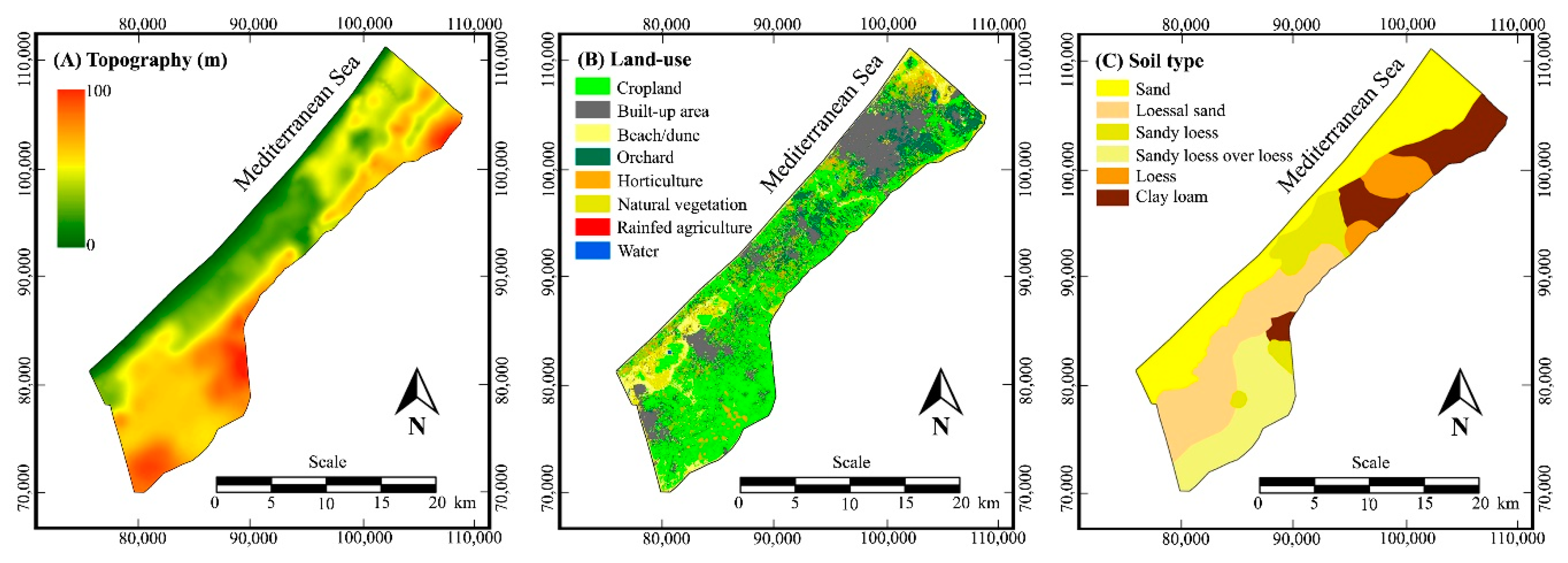
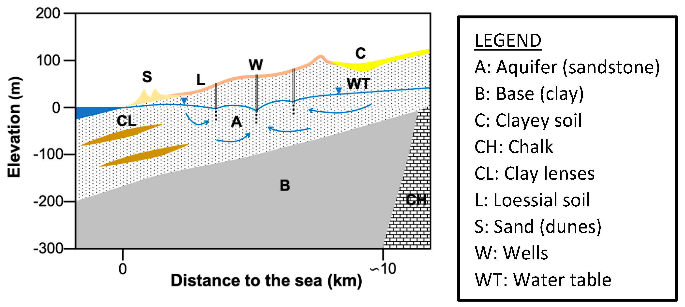
2.1. Study Area and Data

The topography of the Gaza Strip is given in Figure 1A; all maps in this study are in raster format with a resolution of 25 m and elevations are measured above sea level. The topography is characterized by elongated ridges and depressions, which generally extend parallel to the coastline. The ridges and depressions are bisected by the Wadi Gaza, which is mostly dry, and are covered along the coast in the south by shifting sand dunes. The altitude varies from zero on the coast to a maximum of 105 m further inland. A land use map derived from a 2010 SPOT image, obtained from the CLIMB project (7th Framework Programme of the European Commission) [28], shows the spatial distribution of eight land-use classes in the Gaza Strip (Figure 1B). Land-use is predominantly agricultural mixed with urban and built-up areas or nature reserves, mostly beaches and dunes. The major urban areas from north to south are Gaza/Jaballa, Dier al-Balah, Khan Younis and Rafah.

The soil in the Gaza Strip has been classified and mapped into six categories by the Ministry of Planning and International Cooperation (Figure 1C). Along the coast are sandy soils in the form of beaches and sand dunes. Loessial sandy soils exist in the southern part about 5 km inland as a strip parallel to the coast. Sandy loess soils are mixtures of loessial deposits and wind-blown sand and are found mainly in the Wadi Gaza. The sandy loess over loess soils in the southeast are loess soils that are covered with dune sand. Loess soils are found in the south and east of Gaza City. Clay loam alluvial soils are located in the northeastern part of the Gaza Strip. Soil samples were analyzed by Goris and Samain [29] and classified according to the US Department of Agriculture (USDA) textural classification system; three soil texture classes were identified: sand for the sandy soils, sandy loam for the loessial sandy soils and sandy loess soils over loess and sandy clay loam for the sandy loess soils and clay loam soils. Soil samples from loess soils have not been analyzed, but it is likely that the loess soils have a sandy loam texture because they are located between the sandy loess soils and clay loam soils.

The geology of the Gaza Strip is described by Ubeid [30]. There exist no geological or hydrogeological maps of the Gaza Strip, but descriptions of the hydrogeologic conditions have been presented by various authors [21,22,24,25,26,27,31,32]. A schematic hydrogeological cross-section perpendicular to the shoreline is given in Figure 2. The coastal aquifer extends all over the Gaza Strip and consists of calcareous sandstone, referred to as Kurkar, mixed with sand, silt, clay and gravel [21,22,24,26,31]. The thickness of the aquifer varies between 100 m and 200 m along the coast and decreases inland to about 100 m and less along the eastern border. The aquifer is covered with sand dunes near the coast, followed by loessial deposits further inland and clayey soils in the depressions. The impermeable base, referred to as Saqiya Formation, consist mainly of clay [20,25] and limestone [24], with a thickness of 400–1000 m. In the east near the border, the base may also consist of Eocene and Senonian chalk formations [21,26,31]. The coastal aquifer is largely unconfined and, because it is also shallow, contamination from the soil surface is easy [22]. At the coast there are intercalated clay lenses that reach several kilometers inland and divide the aquifer into three sub-aquifers [22,24,26,27,31]. The depth in relation to the water table varies between a few meters in the lowland area along the coast to about 70 m below the surface along the eastern border [31].

Well tests show that the hydraulic conductivity of the coastal aquifer is in the range of 20–80 m/day [31]. Under natural conditions, groundwater flow is towards the Mediterranean Sea, but natural flow patterns have been significantly disturbed by over-extraction from thousands of agricultural and municipal wells scattered throughout the area. More details about the groundwater flow can be found in the literature, e.g., [31,33]. Currently, the depth to groundwater varies from a few meters along the coastline to about 70 m along the eastern border.

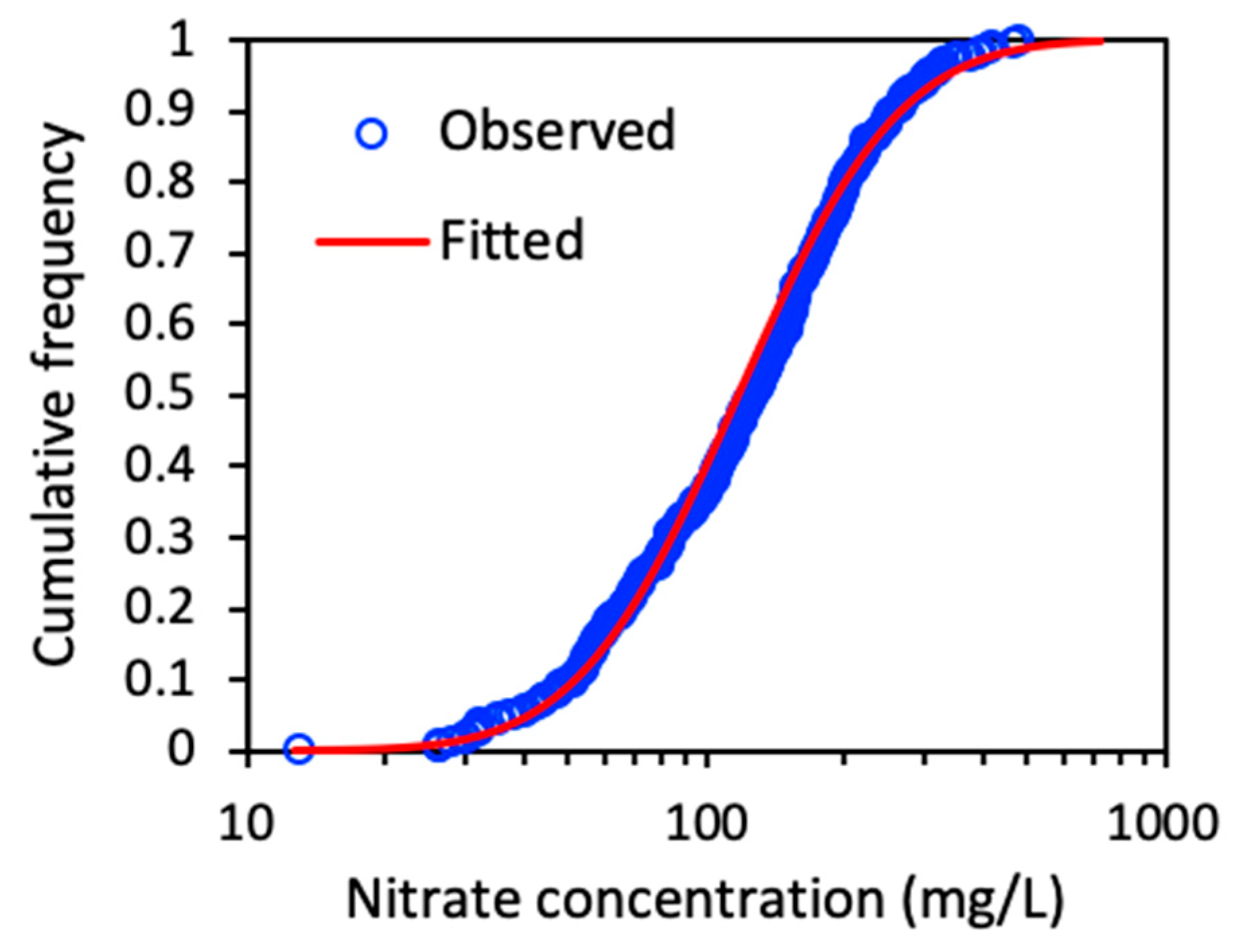
2.2. Data Sampling and Analysis

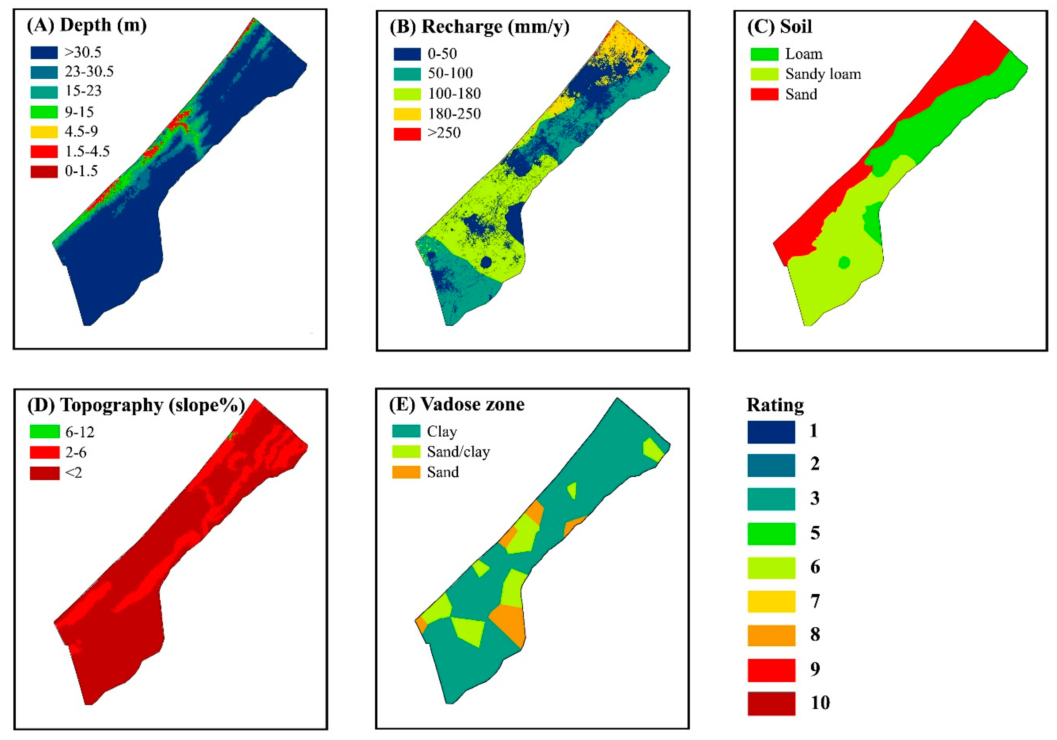
The properties of the vadose zone are derived from 70 well log descriptions provided by the Palestinian Water Authority. The well logs are interpreted as recommended in the DRASTIC manual [4]; 55 are considered to be dominated by clay lenses that restrict transport of contaminants, 10 are dominated by clayey sand and five are primarily sand only. A map of the vadose zone is then obtained by nearest neighbor interpolation.

A map of the groundwater levels is derived from observations in 79 wells by the Palestinian Water Authority in 2015 (Figure 3A). The groundwater levels have been obtained by universal kriging interpolation using a spherical variogram with a range of about 11 km. The results show that natural conditions have been severely disturbed by groundwater abstraction, leading to a large depression of groundwater levels below sea level in the southwest in Rafah and a smaller one in the northeast in Gaza City.

Recharge is a primary source of groundwater, but it is also an important means for pollution transport. Figure 3B shows the groundwater recharge map in the Gaza Strip adapted from Zomlot [34] who estimated the average annual spatial groundwater recharge for the period 1982–2005 using the distributed hydrological WetSpa-Python model. The recharge represents on average about 30% of the precipitation, while the spatial variation of the recharge is clearly controlled by soil type, land-use and precipitation distribution. The highest recharge takes place in the north where rainfall is greater and can easily infiltrate sandy soil. Less recharge occurs in the south where less rainfall falls, in built-up areas with more runoff and in the loess and clay soils areas where infiltration is limited.

One of the main indicators of pollution of the coastal aquifer is nitrate. Groundwater monitoring in the Gaza Strip is conducted by several ministries and coordinated by the Palestinian Water Authority (PWA). Groundwater levels are measured monthly by the PWA in a large number of wells spread across the Gaza Strip. Every summer and winter, the Ministry of Agriculture collects water samples from wells for agricultural use and the Ministry of Health from wells for household use (mostly owned by municipalities) according to standard procedures [35] and the samples are analyzed for several parameters including nitrate according to WHO guidelines [36]. All groundwater and water quality data are transferred to the PWA, Water Resources Department and Gaza Water Data Bank Section, for quality assurance and entry into the hydrologic database.

Figure 3C shows a map of 309 nitrate concentrations observed in 203 wells in April and November–December 2016. Most of these wells have been drilled after 2000 with depths between 60–120 m. The majority of the wells (~90%) are for agricultural use and the remaining are municipal wells used for drinking water production, but the distinction is less strict because agricultural wells with good water quality are often rented by municipalities for domestic use. All wells are shallow in the sense that they tap the upper part of the coastal aquifer. Some wells were measured twice, others only once. The observations are plotted as point values on a background of land-use, simplified into three categories: cultivated, built-up and natural. Unfortunately, the wells are not very uniformly distributed across the study area, as there are not many wells along the coast and in the southeast of the Gaza Strip. The observed nitrate concentration ranges from 13 to 478 mg/L. Figure 4 shows the cumulative frequency distribution, indicating that the data are log-normally distributed. Most nitrate concentrations are well above normal levels, as approximately 90% of the observations are above the WHO standard of 50 mg/L for human consumption. There is no clear pattern in the spatial distribution, but there is a significant correlation with land-use as higher nitrate concentrations are found in urban centers such as Gaza, Dier al-Balah and Rafah and especially in Khan Younis.

2.3. DRASTIC Model

The vulnerability index is obtained by linearly combining the hydrogeological factors using prescribed weights between one and five and the factor classes with prescribed ratings between one and ten, as follows

$$DI={{\displaystyle \sum }}_{i=1}^7\left(a_i{{\displaystyle \sum }}_{j=1}^{n_i}{b}_{ij}{C}_{ij}\right)$$

(1)

where DI is the DRASTIC index, $a_i$ is the weight of factor i, $b_{ij}$ is the rating of class j of factor i, $n_i$ is the number of classes in factor i, and $C_{ij}$ represents class j of factor i. All weights and ratings have been fixed by a panel of experts and should in principle not be changed [4]. The prescribed weights and ratings used in this study are listed in

Table 1. DRASTIC factors with default weights ($a_i$), and factor classes with symbols ($C_{ij}$) and defaults ratings ($b_{ij}$) used to predict the groundwater vulnerability in the Gaza Strip.

Factor	$\mathbf{Weight} \left({\mathit{a}}_{\mathit{i}}\right)$	Class	$\mathbf{Symbol} \left({\mathit{C}}_{\mathit{i}\mathit{j}}\right)$	$\mathbf{Rating} \left({\mathit{b}}_{\mathit{i}\mathit{j}}\right)$
Depth (m)	5	>30.5	C11	1
		23–30.5	C12	2
		15–23	C13	3
		9–15	C14	5
		4.5–9	C15	7
		1.5–4.5	C16	9
		0–1.5	C17	10
Recharge (mm/year)	4	0–50	C21	1
		50–100	C22	3
		100–180	C23	6
		180–250	C24	8
		>250	C25	9
Aquifer	3	Sandstone	C31	6
Soil	2	Loam	C41	5
		Sandy loam	C42	6
		Sand	C43	9
Topography (slope %)	1	6–12	C51	5
		2–6	C52	9
		<2	C53	10
Impact vadose zone	5	Clay	C61	3
		Clayey sand	C62	6
		Sand	C63	8
Conductivity (m/day)	3	20–80	C71	7

.

The factor classes $C_{ij}$ are dichotomous variables that correspond to mappable categories or ranges of a factor. So $C_{ij}$ is one in the area where class j of factor i occurs and zero everywhere else. Note that $C_{ij}$ values are not independent because

$${{\displaystyle \sum }}_{j=1}^{n_i}{C}_{ij}=1$$

(2)

DRASTIC indexes typically range from 65 to 223 [4] (p. 82) and express the potential for groundwater contamination; the higher the value, the more vulnerable.

Sensitivity analysis is used to evaluate the impact of each factor on the overall vulnerability index by deriving an effective weight (adapted from [37]) as

$${\left(a_e\right)}_i=\langle \frac{a_i{b}_{ij}}{DI}\rangle$$

(3)

where ${\left(a_e\right)}_i$ is the relative effective weight (%) of factor i and 〈·〉 stands for the mean value over the study area.

Alternatively, a DRASTIC-N model is used in this study with rating values estimated by multiple linear regression of the log-transformed nitrate concentration with the DRASTIC factor classes extended with land-use factor classes to account for nitrate sources

$$z={\lambda }_0+{{\displaystyle \sum }}_{i=1}^8\left({{\displaystyle \sum }}_{j=2}^{n_i}{\lambda }_{ij}{C}_{ij}\right)$$

(4)

where $z$ is the log-transformed nitrate concentration, ${\lambda }_0$ is the intercept, ${\lambda }_{ij}$ is the regression coefficient of class j of factor i, and $C_{8j}$ represents class j of the land-use factor. Note that the sum over the classes is only for j ≥ 2, because the classes within a factor are not linearly independent; therefore, the first class of each factor is omitted from the equation and its effect is included in the intercept (if $C_{i1}=1$ all other c-values are zero because of Equation (2) and the linear regression given by Equation (4) reduces to $z={\lambda }_0$).

Note that using Equation (4) changes our approach from vulnerability to risk assessment, which also includes pollution hazard, i.e., sources of contamination. Since exact sources of nitrate pollution in the Gaza Strip cannot be quantified on a regional scale, we apply a simplified approach whereby land-use is used as a proxy for hazard, as has been done in many other studies [6,7,8,9,12,13,14,17,18,19,21]. However, to limit the number of variables in the regression equation, we use the simplified land-use map in Figure 3C, with only three land-use classes, i.e., built-up, cultivated and natural. We therefore assume that the nitrate sources in these land-use classes are different, but since the pollution loads are not known exactly, their effect on the nitrate concentration in groundwater is estimated by linear regression.

The regression coefficients are estimated with the lm function of the R Stats package [38]. A DRASTIC-N map is then obtained by applying the linear regression model over the entire study area. Thus, the nitrate concentration values obtained with Equation (4) are used as a substitute for the vulnerability index. Since susceptibility to groundwater contamination is a relative concept, the resulting index values are relative and can be scaled within the normal range of DI values if desired.

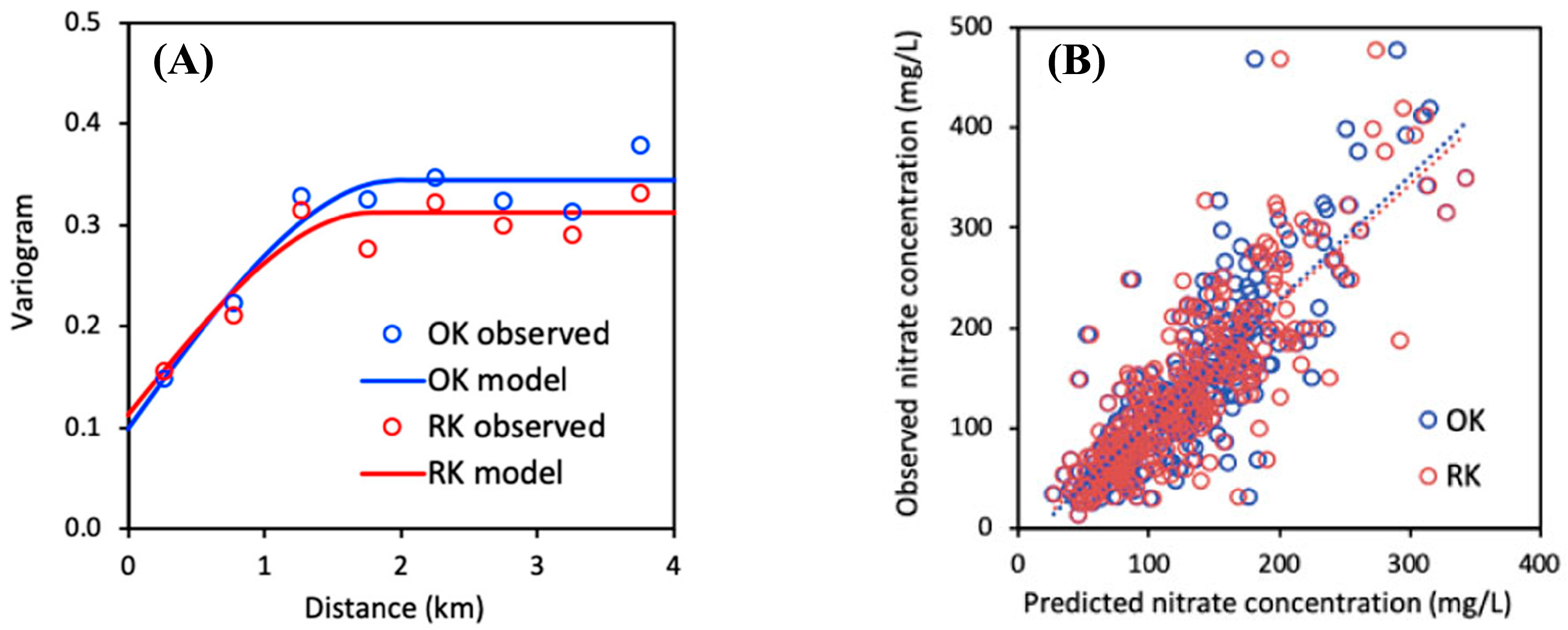
2.4. Geostatistical Analysis

Geostatistical analysis of the log-transformed nitrate concentration includes the derivation of an empirical variogram, fitting by a variogram model, cross-validation of the variogram model and interpolation by kriging to obtain a map of the predicted log-transformed nitrate concentration [39]. Kriging provides the best linear unbiased estimate based on the perceived spatial correlation of the variable concerned [39].

The empirical variogram is fitted by a spherical model

$$\gamma \left(h\right)=\{\begin{array}{ll}0\hfill & h=0\hfill \\ n+\left(s-n\right)(3h/2r-h^3/2r^3)\hfill & 0<h\le r\hfill \\ s\hfill & h>r\hfill \end{array}$$

(5)

where $\gamma$ is the variogram or semi-variance, $h$ is the lag distance, $n$ is the nugget, $s$ is the sill and $r$ is the range. The model parameters $n$, $s$ and $r$ are estimated by the fit.variogram function of the R gstat package for geostatistical data analysis [40]. The variogram model is verified by cross-validation using the krige.cv function of gstat, whereby data points are removed one by one and predicted by kriging using the remaining data.

Mapping of the nitrate concentration is achieved by predicting the log-transformed nitrate concentration using two methods: (1) ordinary kriging

$$z\left(x\right)={{\displaystyle \sum }}_{i=1}^{N\left(x\right)}{w}_{i}z\left(x_i\right)$$

(6)

where $x$ is the location vector, $x_i$ are the locations with observed nitrate concentration, $N\left(x\right)$ is the number of data locations selected within the neighborhood of $x$ and $w_i$ are the kriging weights; and (2) regression kriging

$$z\left(x\right)={{\displaystyle \sum }}_k{\lambda }_k{C}_k\left(x\right)+{{\displaystyle \sum }}_{i=1}^{N\left(x\right)}{w}_i\left[z\left(x_i\right)-{{\displaystyle \sum }}_k{\lambda }_k{C}_k\left(x_i\right)\right]$$

(7)

where $C_k$ are the statistically significant DRASTIC factors and land-use classes and ${\lambda }_k$ are their corresponding regression coefficients, obtained by removing all insignificant factor classes in Equation (4) to obtain a parsimonious regression model.

3. Results

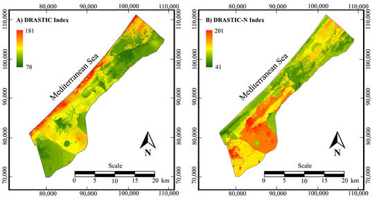
3.1. Groundwater Vulnerability

Table 1 summarizes all factors and classes within a factor, and their standard weights and ratings required to derive a DRASTIC groundwater vulnerability map for the Gaza Strip. The spatial distribution of the factor classes is shown in Figure 5. Note that there is no map for aquifer media and hydraulic conductivity because they are uniform across the study area.

The depth to the groundwater factor map (Figure 5A) is derived from the topographic map (Figure 1A) by subtracting the groundwater level map (Figure 3A). The depth factor in the study area is dominated by the last class indicating groundwater deeper than 30.5 m below the surface, while the other classes are clustered along the coast and in the Gaza Wadi. The recharge factor map (Figure 5B) is derived from the groundwater recharge map (Figure 3B). The recharge factor classes are well distributed across the study area and reflect the impact of soil type and land-use, especially built-up areas. The soil factor map (Figure 5C) is derived from the soil type map (Figure 1C) and shows only three soil factor classes that represent soil texture. The first soil class C₄₁ represents the soils with a sandy clay loam texture but, because this category is not available in the DRASTIC procedure, we opted for the loam class. The topographic factor map (Figure 5D) shows slope classes derived from the topographic map (Figure 1A). There are five topography slope factor classes, but only two are important: slopes less than 2% that correspond to flat areas, and slopes in the range of 2–6% that indicate dunes and ridges. The impact of the vadose zone factor map (Figure 5E) is very patchy due to the nearest neighbor interpolation of the well logs as explained earlier, but the clay class is dominant.

Combination of all factor maps results in a DRASTIC index map as shown in Figure 6A. The DRASTIC index varies between 78 and 181. The scale is in principle relative, but Aller et al. [4] proposed a color key for certain ranges, suggesting that groundwater is very vulnerable when DI ≥ 160 and less vulnerable when DI < 120. For the Gaza Strip, this means that only a few places along the coast are very vulnerable to groundwater contamination, mainly due to the shallow depth to groundwater and sandy soils, while the rest of the Gaza Strip, about 1 km from the coast, is less vulnerable. The latter is mainly due to the clayey nature of the vadose zone and greater depth to the groundwater as a result of over-exploitation of the coastal aquifer. The correlation of the DRASTIC index with the observed nitrate concentration is −0.10 and is therefore not significant.

The results of the parameter sensitivity analysis are shown in

Table 2. Parameter sensitivity results showing theoretical and effective factor weights.

DRASTIC Factor	Relative Weight (%)
	Theoretical	Effective
Depth to groundwater	21.7	8.0
Recharge	17.4	6.6
Aquifer type	13.0	19.0
Soil type	8.7	13.8
Topography (slope)	4.3	10.3
Impact vadose zone	21.7	20.2
Conductivity	13.0	22.1

. The greatest deviations between theoretical and effective factor weights are obtained for the depth to groundwater, recharge, and hydraulic conductivity of the aquifer. For depth and recharge, the effective weight is significantly greater than the theoretical weight, while for conductivity it is the opposite. For depth, the reason is that almost everywhere in the Gaza Strip groundwater is deeper than 30.5 m below the surface, which is considered to be safe with regard to contamination. For recharge, most classes are in the low range, which also implies less vulnerability. For the hydraulic conductivity of the aquifer, there is only one class with a rating on the high side, which results in more vulnerability for the entire Gaza Strip. Therefore, factors with class ratings that deviate systematically from the mean have effective weights that strongly differ from their theoretical value. Comparison of the effective weights between DRASTIC factors, shows that depth to groundwater and recharge are the main factors indicating low vulnerability, while aquifer type, impact of the vadose zone and conductivity are the main factors indicating high vulnerability.

Table 3. DRASTIC factors and land-use classes with estimated coefficients (λ_ij) obtained by linear regression of log-transformed observed nitrate concentration (mg/L); also given are the standard deviation (StD), the t-statistic (t-value) and the probability (p-value) of the estimates; the last column gives the natural exponential of the regression coefficients.

Factor	Class	Symbol	Estimate (λij)	StD	t-Value	p-Value	Exp(λij)
Intercept		λ0	4.66	0.09	54.61	<2 × 10−16	106.
Depth (m)	23–30.5	C12	−0.08	0.15	−0.57	0.57	0.92
	15–23	C13	−0.31	0.18	−1.69	0.09	0.74
	9–15	C14	−0.26	0.33	−0.80	0.42	0.77
	4.5–9	C15	−0.12	0.59	−0.21	0.84	0.88
Recharge (mm/year)	50–100	C22	−0.02	0.29	−0.07	0.95	0.98
	100–180	C23	0.27	0.30	0.90	0.37	1.31
	180–250	C24	0.58	0.33	1.76	0.08	1.78
Soil	Sandy loam	C42	0.36	0.11	3.17	1.7 × 10−3	1.44
	Sand	C43	−0.09	0.09	−0.98	0.33	0.92
Topography (slope %)	<2	C53	0.28	0.08	3.67	2.9 × 10−4	1.32
Vadose zone	Clayey sand	C62	−0.04	0.13	−0.29	0.77	0.96
	Sand	C63	−0.01	0.21	−0.03	0.97	0.99
Land-use	Cultivated	C82	−0.42	0.28	−1.48	0.14	0.66
	Natural	C83	−0.37	0.30	−1.21	0.23	0.69

lists the factors and factor classes and their estimated coefficients obtained by linear regression of the observed log-transformed nitrate concentration with all DRASTIC factors extended with land-use. In addition to the first classes of each factor that are included in the intercept because of the linear dependency of the classes within a factor, some other classes are also not represented because there are no nitrate observations in the areas where these classes occur. This is the case for depth classes 1.5–4.5 m (C₁₆) and 0–1.55 m (C₁₇), recharge class > 250 mm/year (C₂₅) and topography class 6–12% slope (C₅₁); in the latter case topography class 2–6% slope (C₅₂) had to be included instead in the intercept. The significance of the regression predictors is expressed by their t-value and associated p-value, which should normally be less than 5%. It follows that only the intercept and factor classes C₄₂ and C₅₃ are statistically significant, while C₁₃, C₂₄ and C₈₂ are almost significant. In particular, there are no real significant factor classes for impact of the vadose zone. However, it has to be taken into account that 15 regression coefficients are estimated, making the regression model somewhat overfitted. In addition, there may be few observations in small-sized factor classes, leading to more uncertainty in the estimated regression coefficients.

The incorporation of land-use as an additional predictor in the regression equation to account for nitrate hazard seems to have little effect as the significance of the estimated regression coefficients of the land-use classes is rather low. However, closer inspection shows that groundwater recharge is closely related to land-use, especially built-up areas (Figure 3C and Figure 5E). Thus, the effect of land-use on the occurrence of nitrate in groundwater is masked by the recharge factor, resulting in insignificant estimates of the linear regression coefficients of both predictors. The overall regression accuracy is shown in Figure 7, by plotting observed nitrate concentration against nitrate concentration predicted by the regression equation. The predicted values are very discontinuous because they are obtained by combining a limited set of class ratings. Although the deviation with observed nitrate concentration is large, one can clearly distinguish a positive relationship between predictions and observations. The resulting correlation between predicted and observed nitrate concentrations is 0.46, which is low but significant.

The DRASTIC-N index is obtained by using the linear regression equation to combine all DRASTIC factors and land-use classes over the entire study area. For the factor classes that were not included in the regression model because observations in these areas were missing, we assumed the same coefficients as for the nearest class in the same factor. The resulting DRASTIC-N map is shown in Figure 6B. The DRASTIC-N index varies between 41 and 201, which is roughly the same range as the DRASTIC index, so there is no need to rescale the values. The resulting map is quite the opposite to the original DRASTIC index map (Figure 6A), as areas of high and low groundwater vulnerability have been largely swapped. The coastal area appears to be less vulnerable, while the vulnerable areas are further inland. Khan Younis and Dier al-Balah, in particular, appear to be very vulnerable to groundwater pollution, which is consistent with the observed high nitrate concentrations in these areas.

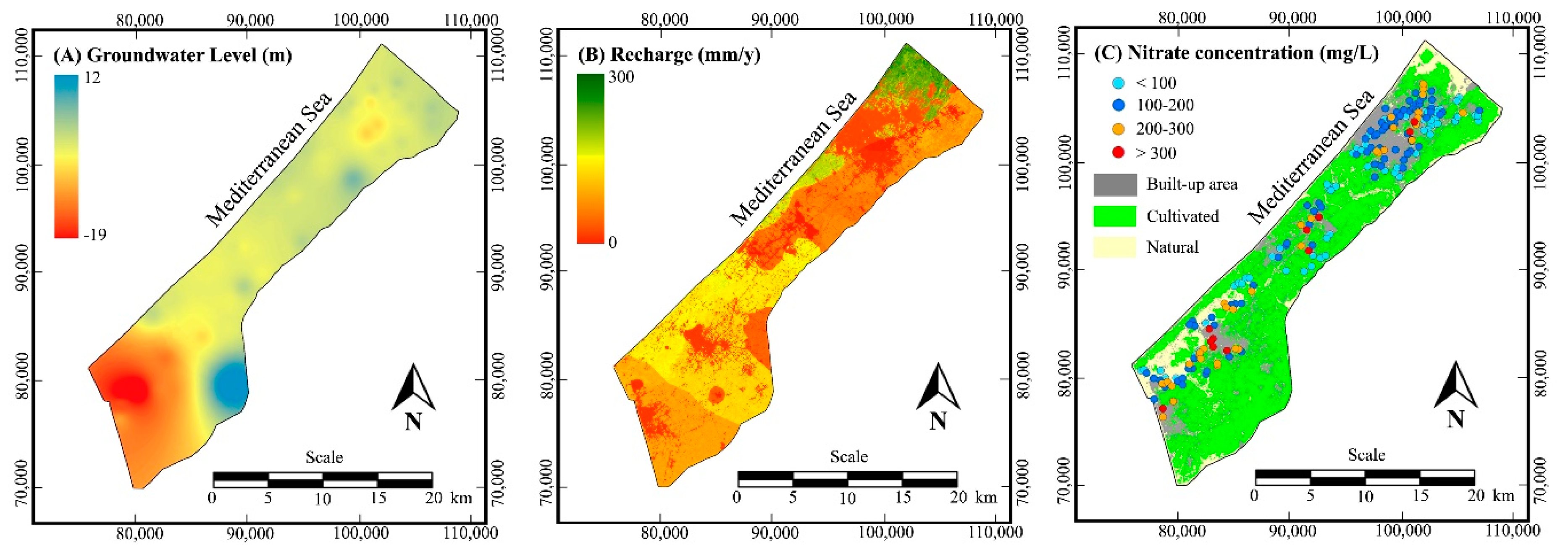
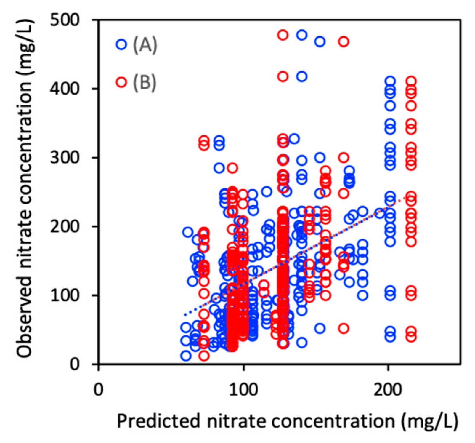
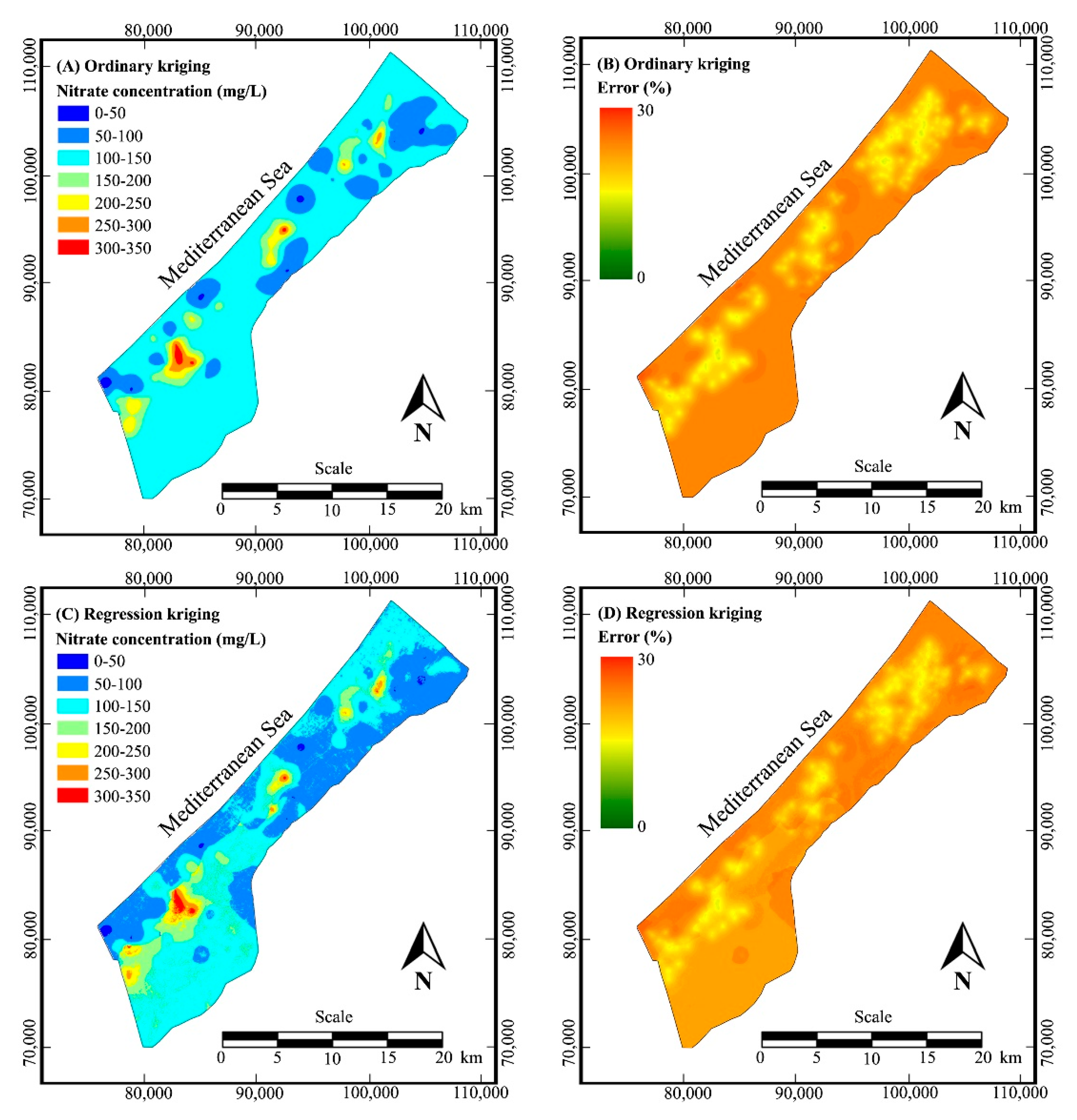
3.2. Mapping of Nitrate Concentration

Figure 8A shows the empirical variogram of the log-transformed nitrate concentration and the fitted spherical model with estimated coefficients given in

Table 4. List of the estimated geostatistical parameters for the spherical variogram model of the log-transformed nitrate concentration in case of ordinary kriging (OK) and regression kriging (RK).

Parameter	OK	RK
Nugget	0.100	0.112
Sill	0.345	0.312
Range (m)	1972	1791

. We also tested other variogram models, such as exponential and Gaussian, but obtained no improvement. The estimated range shows that the nitrate concentration is spatially correlated over a rather small distance of about 2 km. This means that there is little structure in the spatial distribution of the nitrate concentration. The nugget represents about 40% of the sill and can be attributed to measurement errors or to spatial variation on a local scale, smaller than the distance between the wells. The accuracy of the variogram model is verified by cross-validation; results shown in Figure 8B indicate a reasonable agreement between predictions and observations.

Figure 9A shows the map with the spatial distribution of the nitrate concentration obtained by ordinary kriging interpolation. Due to the small range, there is little structure in the spatial distribution of the nitrate concentration, so in most places kriging interpolation only predicts the average log nitrate value, which corresponds to the geometric mean nitrate concentration of 117 mg/L, while locations with higher or lower nitrate concentration appear as isolated spots. In general, such a map does not provide much insight into the spatial distribution of nitrate pollution in the coastal aquifer. Figure 9B shows the relative error map obtained with the ordinary kriging procedure. The relative error is obtained as the ratio of 1.96 times the predicted standard deviation and the predicted value of the log-transformed nitrate concentration [39]. The percentage error values vary between 13 and 27% and are clearly dependent on the distance to the observation points. The further away from the observation points, the greater the error.

The mapping of nitrate concentration is improved by regression kriging using the DRASTIC factors and land-use as external drift components. However, this procedure cannot be performed with all factor classes due to the numerical complexity and computational load. Therefore, less significant factor classes are ignored and a parsimonious linear regression of the log-transformed nitrate concentration is obtained by removing as many classes as possible, including the classes in the intercept, with minimal loss of prediction accuracy. The resulting statistically significant factor classes and their estimated regression coefficients are given in

Table 5. Significant DRASTIC-N factor classes and estimated coefficients (λ_ij) obtained by parsimonious linear regression of log-transformed observed nitrate concentration (mg/L); also given are the standard deviation (StD), the t-statistic (t-value) and the probability (p-value) of the estimates; the last column gives the natural exponential of the coefficient.

Factor	Class	Symbol	Estimate (λij)	StD	t-Value	p-Value	Exp(λij)
Intercept		λ0	4.53	0.06	73.48	<2 × 10−16	93.6
Recharge (mm/year)	180–250	C24	0.45	0.18	2.53	1.2 × 10−2	1.57
Soil	Sandy loam	C42	0.53	0.09	6.09	3.5 × 10−9	1.69
Topography (slope %)	<2	C53	0.24	0.07	3.27	1.1 × 10−3	1.28
Land-use	Built-up area	C81	0.32	0.07	4.52	9.1 × 10−6	1.38

. Only four highly statistically significant factor classes remain: recharge class 180–250 mm/year (C₂₄), soil class sandy loam (C₄₂), topography class slope < 2% (C₅₃) and land-use class built-up area (C₈₁). Note that the land-use class built-up area (C₈₁) is very significant with a p-value of about 1 × 10⁻⁵, which is a result of deleting the less significant recharge classes (C₂₁, C₂₂ and C₂₃) that interfered with the built-up land-use class. Also recharge class 180–250 mm/year (C₁₃) is now statistically significant with a p-value of 0.001, because other less significant classes that interfered with this class are ignored. The correlation between nitrate predictions and observations is 0.46, which is the same as obtained with the full linear regression. Figure 8A shows the empirical variogram and the fitted spherical model with estimated coefficients given in Table 5 in case of regression kriging. The variogram model and its parameters are very close to what is obtained for ordinary kriging, except that the sill is somewhat smaller. This shows that by including external drift components, the interpolation of the nitrate concentration becomes more accurate and the spatial variability of the nitrate distribution becomes less uncertain. The accuracy of the variogram model is also verified by cross-validation with similar results as for ordinary kriging (Figure 8B).

Figure 9C shows the resulting map with the spatial distribution of the nitrate concentration obtained by regression kriging interpolation. This map shows much more detail than the previous map obtained by ordinary kriging (Figure 9A). One notices in particular the effect of urban areas, of soil texture in the southeast and of topography along the coast and northeast of the Gaza Strip. Figure 9D shows the corresponding relative error map obtained with the regression kriging procedure. The values also vary between 13% and 27% but are on average slightly lower than the errors obtained by ordinary kriging (Figure 9B). The error values also strongly depend on the distance from the observation points but are also influenced by the DRASTIC factors and land-use classes used in the estimation procedure.

4. Discussion

4.1. DRASTIC Groundwater Vulnerability

The DRASTIC index map shown in Figure 6A is very similar to what has been presented in other studies conducted for the Gaza Strip. Baalousha [21] obtained DI values between 75 to 135. The highest values were obtained in the northwest along the coast, where the topsoil is sand and recharge is highest. The lowest values were found in the northeast where the soil is clayey and in the southeast where the recharge is very low. Baalousha [21] concluded that most of the Gaza Strip is only moderately vulnerable. Almasri [9] obtained DI values between 80 and 180 and concluded that high vulnerability zones are located only along the coast and the rest of the Gaza Strip is moderately vulnerable. Al Hallaq and Elaish [22] obtained DI values between 88 and 190 for the Khan Younis Governorate of the Gaza Strip; the highest values occurred along the coast where the groundwater is shallow and soil is very permeable, while further inland the vulnerability to contamination is moderate to low. In all of these studies, the DRASTIC factor weights and class ratings were adjusted according to the authors’ discretion, yet all findings are consistent with what was obtained in this study using the standard DRASTIC procedure. One may therefore wonder whether it is necessary to adapt the DRASTIC procedure to local circumstances.

The DI values obtained with DRASTIC in this study do not correspond to the observed nitrate concentration in groundwater. Baalousha [21] and Almasri [9] came to the same conclusion for the Gaza Strip. However, this lack of correlation between DI and nitrate does not mean that there is no relationship between occurrence of nitrate and DRASTIC factors. Several studies have also recommended including land-use in the DRASTIC procedure to improve correlation with occurrence of nitrate [6,11,12,16,41]. Indeed, the DRASTIC vulnerability map does not necessarily relate to nitrate contamination in groundwater because vulnerability only takes into account natural intrinsic factors that make an aquifer susceptible to pollution and does not depend on the likelihood of sources of contamination. Therefore, the risk of groundwater contamination by nitrate is determined by a combination of aquifer vulnerability and contamination hazard. However, nitrate hazard in the Gaza Strip is not well known and is difficult to assess in practice. Therefore, land-use is used as a proxy for nitrate hazard, whereby we intrinsically assume that nitrate sources within a land-use class are diffuse. Thus, in this study, multiple linear regression of log-transformed nitrate concentration shows significant relationships between different DRASTIC factors in combination with land-use and the presence of nitrate in groundwater.

The degree of association is given by the regression coefficients shown in Table 3. The physical interpretation is revealed by the natural exponential of these coefficients in the last column of the table. The natural exponential of the intercept, exp(${\lambda }_0$), gives the expected nitrate concentration in an area with site-specific features corresponding to factor classes omitted in the regression equation due to interdependence between factor classes. When one of these site-specific characteristics is exchanged for another factor class, C_ij, the resulting nitrate level is obtained by multiplying exp(${\lambda }_0$) and the exponential of the regression coefficient of that factor class, exp(${\lambda }_{ij}$). So, exp(${\lambda }_{ij}$) values larger than one increase the nitrate level and vice-versa. Factor classes that promote groundwater contamination by nitrate are high recharge (C₂₃ and C₂₄), sandy loam soil (C₄₂) and flat areas (C₅₃), and factor classes associated with less nitrate contamination are small depth to groundwater (C₁₂–C₁₅), less recharge (C₂₂) and cultivated or natural land-use (C₈₂ and C₈₃). Note that the vadose zone has almost no impact. Not all of these findings are statistically significant considering their p-value, but this is mainly due to lack of data. The physical interpretation is mostly obvious. High recharge (C₂₄), sandy loam soil (C₄₂) and flat areas (C₅₃) increase nitrate in groundwater because they promote and increase seepage from sewage and fertilization, and the inverse applies to less recharge (C₂₂). The effect of a smaller depth to groundwater (C₁₂–C₁₅) is less clear. One would expect a positive effect on nitrate content in groundwater, but the opposite is true. The reason must be found in the spatial appearance of these classes; they are all located along the coast and in the Gaza Wadi (Figure 5A), where observed nitrate concentrations are generally low, which may be due to less agricultural activity in dunes and on beaches and on the sandy soils along the coast. It is also necessary to clarify the conclusion that cultivated or natural land leads to less nitrate pollution. This finding should be seen in contrast to the land-use class in the predictor, which is built-up area. Our results thus show that nitrate in groundwater in urban areas is higher than in other areas, which is in line with what is observed in practice and indicates more nitrate hazard in urban areas.

The method used in this study to determine relationships between DRASTIC factors with land-use and the occurrence of nitrate in groundwater has a number of advantages over other techniques reported in the literature, because: (1) all class ratings are modified while other studies have only adjusted the factor weights [6,14]; (2) all nitrate data is used without loss of information, while other studies only use ranked data or data above a certain threshold [6,8,13,14,16]; (3) we applied multivariate statistical analysis, while other studies used only univariate techniques such as Spearman’s rank correlation or weights of evidence [8,17].

4.2. Nitrate Concentration Maps

Groundwater nitrate concentration maps for the Gaza Strip presented by Shomar et al. [25], Baalousha [26] and Almasri and Ghabayen [27] are similar to the map obtained by ordinary kriging in this study (Figure 9A). However, these maps do not provide much insight into the spatial distribution of nitrate occurrence or factors affecting nitrate content, except that higher nitrate concentrations are found in urban centers, especially in Khan Younis. Nitrate maps from other studies such as Huan et al. [14] and Nadiri et al. [20] are similar in this regard. The likely reason is that nitrate contamination is strongly determined by local conditions, which is reflected by the small autocorrelation range and large nugget of the variogram found in this study. It is therefore important to develop other techniques to improve the derivation of such maps and find ways to link the nitrate distribution to external explanatory factors. Our approach to using DRASTIC factors and land-use as drift components for regression kriging of nitrate concentration is original in this regard. The results show that mapping of the spatial distribution of the nitrate concentration in groundwater in the Gaza Strip can be improved by considering groundwater recharge, topography, soil type and land-use as indicators of spatial variations in occurrence of nitrate. No such relationships have been previously reported; Shomar et al. [25] only reported that nitrate comes mainly from manure, Baalousha [26] concluded that nitrate contamination in groundwater is mainly due to leakage from wastewater, cesspools and over-loaded treatment plants, and Almasri and Ghabayen [27] concluded that most elevated nitrate concentrations occur in urban areas and intensive agricultural areas.

When the map obtained by regression kriging interpolation is compared with the map obtained by ordinary kriging interpolation (Figure 9A,C), several contrasts and details stand out as one can distinguish topographic ridges, soils types, built-up areas, etc., which were previously not noticeable. These environmental factors apparently play a role in the occurrence and spatial distribution of the presence of nitrate in groundwater. The error maps (Figure 9B,D) also indicate the influence of explanatory factors for predicting the nitrate concentration. In places where significant additional information is available, for example sandy loam soil in the southeast of the Gaza Strip, the error obtained with regression kriging is smaller than the error obtained with ordinary kriging.

However, it should be taken into account that the relationships between the occurrence of nitrate and site-specific features have been identified by statistical analysis, and while physical reasons may seem obvious for some of these relationships, the reality may be more complicated. For example, the impact of groundwater recharge is related to land-use and soil types and topography may correlate with agricultural practices. The spatial appearance of nitrate in groundwater can therefore be a combination and interaction of various causative factors. We also recognize that the quantity and quality of the data used in this study are inadequate in several respects; for example the nitrate observations are not well distributed over the study area, the spatial distribution of hydrogeological properties is not sufficiently detailed, effects from several site-specific properties cannot be evaluated because no nitrate observations are available in these areas and the effects of many site specific properties are not statistically significant due to insufficient observations of nitrate levels.

In the Gaza Strip, all groundwater contamination by nitrate is attributable to activities at the soil surface. These mainly consist of so-called point sources such as leakage of wastewater from cesspools, landfills, over-loaded treatment plants, non-sewered areas and industrial discharges, and to a lesser extend of diffuse sources, mainly excessive use of nitrogen fertilizers in agriculture, which are leached by rain infiltration, and excessive irrigation [21]. Leaked wastewater and leaching are rich in nitrogen, which is decomposed into nitrate under aerobic conditions in the topsoil. Nitrate is highly soluble and is not normally highly adsorbed by the soil. It therefore seeps down through the vadose zone with a travel time determined by the permeability, the amount of recharge and the depth to the water table [24,25,27]. Since the coastal aquifer is shallow and unconfined, nitrate penetrates into the groundwater and causes nitrate pollution [21]. The resulting nitrate concentration in the aquifer is further influenced by advection and dispersion with the groundwater flow. Normally the regional groundwater flow is towards the Mediterranean, but the natural flow patterns are disturbed by a large number of pumping wells widely distributed over the Gaza Strip. There is also little vertical downward flow because the wells are mainly located in the upper part of the aquifer [27]. Nitrate concentrations observed in wells are thus the result of converging groundwater flows, ultimately from the nitrate sources near the wells, and thus represent local conditions. This can also be seen on the nitrate concentration maps, where the highest concentrations are noted in urban areas such as Gaza, Dier al-Balah, Khan Younis and Rafah, in which nitrate sources are abundant. This also explains why the local topography, recharge rates and soil types can be used as significant predictors of nitrate mapping by regression kriging.

5. Conclusions

The groundwater vulnerability map of the Gaza Strip, derived using the standard DRASTIC procedure with seven hydrogeological factors and default weight and rating values, shows that only a small zone along the coast is very vulnerable due to the shallow groundwater depth and sandy soil, while further inland the groundwater is less vulnerable due to the clayey nature of the vadose zone and the greater depth to the groundwater resulting from over-exploitation of the aquifer. This map is very similar to what has been presented in other similar studies. However, no correlation can be detected with the observed nitrate concentration in groundwater.

An improved DRASTIC-N model is obtained by multiple linear regression of observed log-transformed nitrate concentration, demonstrating significant relationships between some DRASTIC factors combined with land-use and the occurrence of nitrate in groundwater. Factors that promote groundwater contamination by nitrate include high groundwater recharge, sandy loam soil and flat terrain, leading to more seepage from waste, wastewater and fertilizers. Factors that cause less nitrate pollution are ridge slopes and less groundwater recharge, which reduce seepage. No significant effect of the vadose can be detected. Including land-use as an additional predictor in the regression equation shows that nitrate hazard in built-up areas is greater than in cultivated or natural land. The current method for determining relationships between DRASTIC factors and the occurrence of nitrate in groundwater has a number of advantages over other techniques reported in the literature, as the method uses multivariate statistical analysis of all factors and nitrate data without loss of information. Application of the linear regression model over the entire study area results in a groundwater vulnerability map, which is opposite to the original DRASTIC map, since coastal areas are considered less vulnerable, while groundwater vulnerability is higher inland.

Geostatistical analysis shows that the nitrate concentration is strongly determined by local conditions and is only spatially correlated over a narrow range of about 2 km. Therefore, a map of the nitrate concentration obtained by ordinary kriging interpolation shows only isolated spots with high or low nitrate levels. An improved map is obtained by regression kriging using the most significant classes of groundwater recharge, topography, soil type and land-use, as indicators of the spatial variations in nitrate occurrence. The map obtained by regression kriging interpolation reveals more environmental factors such as dunes, ridges, soils types and built-up areas, that influence the occurrence of nitrate in groundwater.

The resulting groundwater vulnerability and nitrate distribution maps generated in this study could be useful to the relevant authorities and decision-makers responsible for groundwater management in the Gaza Strip, Palestine. In addition, the proposed analyses techniques to improve groundwater vulnerability and nitrate contamination mapping may inspire other studies investigating similar problems. However, it is recommended that a thorough interpretation of these results in order to improve the management of the groundwater resources in the Gaza Strip requires more detailed information on the geological and hydrogeological conditions and in particular on the sources of groundwater pollution and groundwater extraction rates and the effects on groundwater drawdowns and groundwater flows.

References

1. Efron, S.; Fischbach, J.R.; Blum, I.; Karimov, R.I.; Moore, M. The Public Health Impacts of Gaza’s Water Crisis Analysis and Policy Options; RAND Corporation: Santa Monica, CA, USA, 2018; p. 87. [Google Scholar] [CrossRef] [Green Version]
2. World Bank. Securing Water for Development in West Bank and Gaza; International Bank for Reconstruction and Development: Washington, DC, USA, 2018; p. 30. [Google Scholar]
3. Machiwal, D.; Jha, M.K.; Singh, V.P.; Mohan, C. Assessment and Mapping of Groundwater Vulnerability to Pollution: Current Status and Challenges. Earth-Sci. Rev. 2018, 185, 901–927. [Google Scholar] [CrossRef]
4. Aller, L.; Bennet, T.; Lehr, J.H.; Petty, R.J.; Hackett, G. DRASTIC: A Standardized System for Evaluating Groundwater Pollution Potential Using Hydrogeologic Settings; Doc. EPA/600/2-87/035; United States Environmental Protection Agency (USEPA): Washington, DC, USA, 1987; p. 622.
5. Shirazi, S.M.; Imran, H.M.; Akib, S. GIS-based DRASTIC method for groundwater vulnerability assessment: A review. J. Risk Res. 2012, 15, 991–1011. [Google Scholar] [CrossRef]
6. Stigter, T.Y.; Ribeiro, L.; Carvalho Dill, A.M. Evaluation of an intrinsic and a specific vulnerability assessment method in comparison with groundwater salinisation and nitrate contamination levels in two agricultural regions in the south of Portugal. Hydrogeol. J. 2006, 14, 79–99. [Google Scholar] [CrossRef]
7. Panagopoulos, G.P.; Antonakos, A.K.; Lambrakis, N.J. Optimization of the DRASTIC method for groundwater vulnerability assessment via the use of simple statistical methods and GIS. Hydrogeol. J. 2006, 14, 894–911. [Google Scholar] [CrossRef]
8. Antonakos, A.; Lambrakis, N. Development and testing of three hybrid methods for the assessment of aquifer vulnerability to nitrates, based on the drastic model, an example from NE Korinthia, Greece. J. Hydrol. 2007, 333, 288–304. [Google Scholar] [CrossRef]
9. Almasri, M.N. Assessment of intrinsic vulnerability to contamination for Gaza coastal aquifer, Palestine. J. Environ. Manag. 2008, 88, 577–593. [Google Scholar] [CrossRef] [PubMed]
10. Assaf, H.; Saadeh, M. Geostatistical assessment of groundwater nitrate contamination with reflection on DRASTIC vulnerability assessment: The case of the Upper Litani Basin, Lebanon. Water Resour. Manag. 2009, 23, 775–796. [Google Scholar] [CrossRef]
11. Arauzo, M. Vulnerability of groundwater resources to nitrate pollution: A simple and effective procedure for delimiting Nitrate Vulnerable Zones. Sci. Total Environ. 2017, 575, 799–812. [Google Scholar] [CrossRef] [PubMed]
12. Thirumalaivasan, D.; Karmegam, M.; Venugopal, K. AHP-DRASTIC: Software for specific aquifer vulnerability assessment using DRASTIC model and GIS. Environ. Modell. Softw. 2003, 18, 645–656. [Google Scholar] [CrossRef]
13. Dixon, B. A case study using support vector machines, neural networks and logistic regression in a GIS to identify wells contaminated with nitrate-N. Hydrogeol. J. 2009, 17, 1507–1520. [Google Scholar] [CrossRef]
14. Huan, H.; Wang, J.; Teng, Y. Assessment and validation of groundwater vulnerability to nitrate based on a modified DRASTIC model: A case study in Jilin City of northeast China. Sci. Total Environ. 2012, 440, 14–23. [Google Scholar] [CrossRef] [PubMed]
15. Fijani, E.; Nadiri, A.A.; Moghaddam, A.A.; Tsai, F.T.C.; Dixon, B. Optimization of DRASTIC method by supervised committee machine artificial intelligence to assess groundwater vulnerability for Maragheh–Bonab plain aquifer, Iran. J. Hydrol. 2013, 503, 89–100. [Google Scholar] [CrossRef]
16. Pacheco, F.A.L.; Pires, L.M.G.R.; Santos, R.M.B.; Sanches Fernandes, L.F. Factor weighting in DRASTIC modeling. Sci. Total Environ. 2015, 505, 474–486. [Google Scholar] [CrossRef] [PubMed]
17. Kazakis, N.; Voudouris, K. Groundwater vulnerability and pollution risk assessment of porous aquifers to nitrate: Modifying the DRASTIC method using quantitative parameters. J. Hydrol. 2015, 525, 13–25. [Google Scholar] [CrossRef]
18. Bonfanti, M.; Ducci, D.; Masetti, M.; Sellerino, M.; Stevenazzi, S. Using statistical analyses for improving rating methods for groundwater vulnerability in contamination maps. Environ. Earth Sci. 2016, 75, 1003. [Google Scholar] [CrossRef] [Green Version]
19. Jang, C.; Lin, C.; Liang, C.; Chen, J.S. Developing a reliable model for aquifer vulnerability. Stoch. Environ. Res. Risk Assess. 2016, 30, 175–187. [Google Scholar] [CrossRef]
20. Nadiri, A.A.; Sedghi, Z.; Khatibi, R.; Gharekhani, M. Mapping vulnerability of multiple aquifers using multiple models and fuzzy logic to objectively derive model structures. Sci. Total Environ. 2017, 593–594, 75–90. [Google Scholar] [CrossRef] [PubMed]
21. Baalousha, H. Vulnerability assessment for the Gaza Strip, Palestine using DRASTIC. Environ. Geol. 2006, 50, 405–414. [Google Scholar] [CrossRef]
22. Al Hallaq, A.H.; Elaish, B.S.A. Assessment of aquifer vulnerability to contamination in Khanyounis Governorate, Gaza Strip—Palestine, using the DRASTIC model within GIS environment. Arab. J. Geosci. 2012, 5, 833–847. [Google Scholar] [CrossRef]
23. Wick, K.; Heumesser, C.; Schmid, E. Groundwater nitrate contamination: Factors and indicators. J. Environ. Manag. 2012, 111, 178–186. [Google Scholar] [CrossRef] [Green Version]
24. Abu Maila, Y.A.; El-Nahal, I.; Al-Agha, M.R. Seasonal variations and mechanisms of groundwater nitrate pollution in the Gaza Strip. Environ. Geol. 2004, 47, 84–90. [Google Scholar] [CrossRef]
25. Shomar, B.; Osenbrück, K.; Yahya, A. Elevated nitrate levels in the groundwater of the Gaza Strip: Distribution and sources. Sci. Total Environ. 2008, 398, 164–174. [Google Scholar] [CrossRef]
26. Baalousha, H. Analysis of nitrate occurrence and distribution in groundwater in the Gaza Strip using major ion chemistry. Global NEST J. 2008, 10, 337–349. [Google Scholar]
27. Almasri, M.N.; Ghabayen, S.M.S. Analysis of nitrate contamination of Gaza coastal aquifer, Palestine. J. Hydrol. Eng. 2008, 13, 132–140. [Google Scholar] [CrossRef]
28. Ludwig, R.; Soddu, A.; Duttmann, R.; Baghdadi, N.; Benabdallah, S.; Deidda, R.; Marrocu, M.; Strunz, G.; Wendland, F.; Engin, G.; et al. Climate-induced changes on the hydrology of Mediterranean basins—A research concept to reduce uncertainty and quantify risk. Fresen. Environ. Bull. 2010, 19, 2379–2384. [Google Scholar]
29. Goris, K.; Samain, B. Sustainable Irrigation in the Gaza Strip. M.Sc. Thesis, Katholieke Universiteit Leuven, Leuven, Belgium, 2001; p. 156. [Google Scholar]
30. Ubeid, K.F. The nature of the Pleistocene-Holocene palaeosols in the Gaza Strip, Palestine. Geologos 2011, 17, 163–173. [Google Scholar] [CrossRef] [Green Version]
31. Qahman, K.; Larabi, A. Evaluation and numerical modeling of seawater intrusion in the Gaza aquifer, Palestine. Hydrogeol. J. 2006, 14, 713–728. [Google Scholar] [CrossRef]
32. Mushtaha, A.M.; Van Camp, M.; Walraevens, K. Evolution of runoff and groundwater recharge in the Gaza Strip over the last four decades. Environ. Earth Sci. 2019, 78, 32. [Google Scholar] [CrossRef]
33. Aish, A.M. Hydrogeological Study and Artificial Recharge Modeling of the Gaza Coastal Aquifer Using GIS and MODFLOW. Ph.D. Thesis, Vrije Universiteit Brussel, Brussels, Belgium, 2004; p. 169. [Google Scholar]
34. Zomlot, Z. Spatial and Temporal Estimation of Groundwater Recharge: Identifying Controlling Factors and Impact Assessment. Ph.D. Thesis, Vrije Universiteit Brussel, Brussels, Belgium, 2015; p. 173. [Google Scholar]
35. APHA. Standard Methods for the Examination of Water and Wastewater, 21th ed.; American Public Health Association: Washington, DC, USA, 2005; p. 1368. [Google Scholar]
36. Bartram, J.; Ballance, R. Water Quality Monitoring—A Practical Guide to the Design and Implementation of Freshwater Quality Studies and Monitoring Programs; World Health Organization, United Nations Environment Programme, E. & F.N. Spon: London, UK, 1996; p. 396. [Google Scholar]
37. Babiker, I.S.; Mohammed, M.A.A.; Hiyama, T.; Kato, K. A GIS-based DRASTIC model for assessing aquifer vulnerability in Kakamigahara Heights, Gifu Prefecture, central Japan. Sci. Total Environ. 2005, 345, 127–140. [Google Scholar] [CrossRef] [PubMed]
38. R Core Team. R: A Language and Environment for Statistical Computing; R Foundation for Statistical Computing: Vienna, Austria, 2018; Available online: http://www.R-project.org/ (accessed on 28 October 2019).
39. Goovaerts, P. Geostatistics for Natural Resources Evaluation; Oxford University Press: New York, NY, USA, 1997; p. 483. [Google Scholar]
40. Pebesma, E.J. Multivariable geostatistics in S: The gstat package. Comput. Geosci. 2004, 30, 683–691. [Google Scholar] [CrossRef]
41. Catani, V.; Zuzolo, D.; Esposito, L.; Albanese, S.; Pagnozzi, M.; Fiorillo, F.; de Vivo, B.; Cicchella, D. A New Approach for Aquifer Vulnerability Assessment: The Case Study of Campania Plain. Water Resour. Manag. 2020, 34, 819–834. [Google Scholar] [CrossRef]
Figure 1. Maps of the Gaza Strip showing topography (A), land-use (B), and soil types (C).
Water 12 02022 g001
Figure 2. Schematization of the hydrogeological cross-section of the Gaza aquifer (adapted from [31,32]).
Water 12 02022 g002
Figure 3. Maps showing observed groundwater level in 2015 (A), estimated groundwater recharge (adapted from Zomlot [34]) (B), and observed groundwater nitrate concentration in 2016 (C).
Water 12 02022 g003
Figure 4. Cumulative frequency distribution of the observed groundwater nitrate concentration and fitted lognormal distribution.
Water 12 02022 g004
Figure 5. Spatial distribution of the DRASTIC factors: depth to the groundwater (A), groundwater recharge (B), soil texture (C), topographic slope (D), and impact of the vadose zone (E); also shown is the color scale for the rating values.
Water 12 02022 g005
Figure 6. Maps of DRASTIC index obtained by the standard procedure and ratings (A), and DRASTIC-N index obtained by multiple linear regression of observed log-transformed nitrate concentration with DRASTIC factors and land-use (B).
Water 12 02022 g006
Figure 7. Observed nitrate concentration versus nitrate concentration predicted by linear regression with all DRASTIC factors and land-use classes (A), and with statistically significant DRASTIC factors and land-use classes (B).
Water 12 02022 g007
Figure 8. Empirical variograms of log-transformed nitrate concentration and fitted spherical models (A), and cross-validation of the variogram models (B), for ordinary kriging (OK) and regression kriging (RK).
Water 12 02022 g008
Figure 9. Spatial distribution of nitrate concentration (A) and the corresponding relative error (B) obtained by ordinary kriging interpolation, and nitrate concentration (C) and corresponding relative error (D) obtained by regression kriging interpolation.
Water 12 02022 g009