Beyond Human Interventions on Complex Bays: Effects on Water and Wave Dynamics (Study Case Cádiz Bay, Spain)

Abstract

Bays are coastal environments with significant socio-economic importance, which has led to the development of human interventions in their interior that can have an important impact on the water and wave dynamics, which in turn modify their morphodynamics and water renewal capacity. In order to deepen our understanding of these impacts, numerical modeling was used in a bay in southern Spain to analyze the effect of inner harbor expansion and channel deepening, including the baroclinic and wave propagation effects, as well as variations in salinity and temperature. The results show that the deepening of the channel decreases the amplitude and speed of the tidal wave as it propagates through the bay, reducing the effects of friction and increasing the flushing time. The system evolves from convergent to a damping system that can potentially reduce the effects produced by projected sea level rise. In addition, the seasonal variability of salinity and temperature is reduced, increasing the bed shear stresses and resulting in increased turbidity that can affect the biogeochemistry of the bay. Finally, wave heights decrease along the main waterway, although the yearly-average wave energy flux is only slightly modified on the interior beaches of the bay. However, significant variations are observed during storms, which could affect the morphodynamics of these beaches.

1. Introduction

Tidal environments such as bays and estuaries are highly valuable ecosystems that often host densely populated areas. Like any coastal system, their evolution depends on the interaction between natural processes, human activities and the hydrodynamic and morphodynamic response to these activities [1]; therefore, their current behaviour is strongly conditioned and is a consequence of human interventions of different types carried out during the last decades or even centuries [2]. Actually, human action is the main reason for the recent changes observed for estuaries and bays [3]. Natural processes are usually dominated by complex, multi-scale and non-linear dynamic interactions between different agents such as astronomical tides and storm surge, waves, baroclinic flows, wind, sediment transport and in some cases river discharges [4]. In the case of human activities, such as maintenance and deepening of waterways or extensions of port areas, their effects on estuaries and bays can dramatically alter the hydrodynamic forcings, and consequently, the ecological status of these dynamic systems [1].

These impacts lead to a struggle between the development of economic activities and the preservation of the environment integrity [5,6], which has led to an increasing need to identify, reduce or remedy the long-term adverse effects of human activities on the ecosystems of bays and estuaries [7]. Therefore, for a sustainable management of these systems that maintains their ecological and recreational functions, but at the same time favors economic development, a deep knowledge of their hydrodynamics and morphodynamics is required, as well as the identification and quantification of the effects of human interventions [8].

In recent years, numerous studies have been carried out in bays and estuaries in which impacts of human activities have been identified and characterized, such as those on the tidal amplitudes [9,10,11,12], nutrient transport [13] and morphodynamics [14,15,16]. Many of these analyses have been carried out using: (1) idealized box models based on volumetric changes [2,14,17,18]; or (2) numerical simulations of the changes expected after the implementation of human interventions with process-based models [1,12,16]. The main drawback of the latter is that these simulations require extensive calibration and validation which is not easy to perform [5]. However, there are still some aspects of the dynamics of these systems that have not been analyzed in depth, despite the fact that a significant number of the world’s main bays and estuaries are made up of interconnected basins, including the San Francisco Bay [19,20], the Chesapeake Bay [21], the Yangtze River estuary [22,23] or the Harvey River estuary [24].

In particular, the effects on wave propagation and on the capacity of the interconnected basins to maintain the water renewal have received much less attention from researchers. The assessment of these impacts is especially relevant in estuarine systems with basins characterized by different geometries and hydro-morphodynamic behaviors. An example of these systems is the Cádiz Bay (southern Spain), formed by five different basins ranging from open water bodies directly connected to the open sea to shallow tidal creek systems dominated by friction. In recent years, a new container terminal has been built to increase the commercial capacity of the Port of Cádiz Bay, which will involve also the deepening of the main navigation channel. Although previous studies analyzed the variations in the characteristics of the tidal wave, the residual currents [12,25] and the morphodynamics [25,26] caused by these interventions, in none of them have the effects of the waves and the variations caused by changes in the density and temperature of the water been considered, nor have the changes in the water renewal capacity in the affected basins.

The main objective of this work is to analyze the impact of the recent human interventions developed at Cádiz Bay on the water renewal capacity, the temperature and salinity distributions and the propagation of waves and their morphodynamic consequences. The methodology is based on the numerical simulation of the same complete year for pre- and post-intervention scenarios using a model calibrated and validated for hydrodynamics and salinity and temperature transports. The results are also used to analyze the variations of the bed shear stresses, as well as the wave energy flux that reach the inner beaches of the bay and determine the evolution of their plain-view. The results obtained are of interest to scientists and managers who analyze the effects of human interventions in similar bays where port extensions or deepening of navigation channels are carried out. The analysis of these effects is even more important due to the effects that global warming will have on these environments [27].

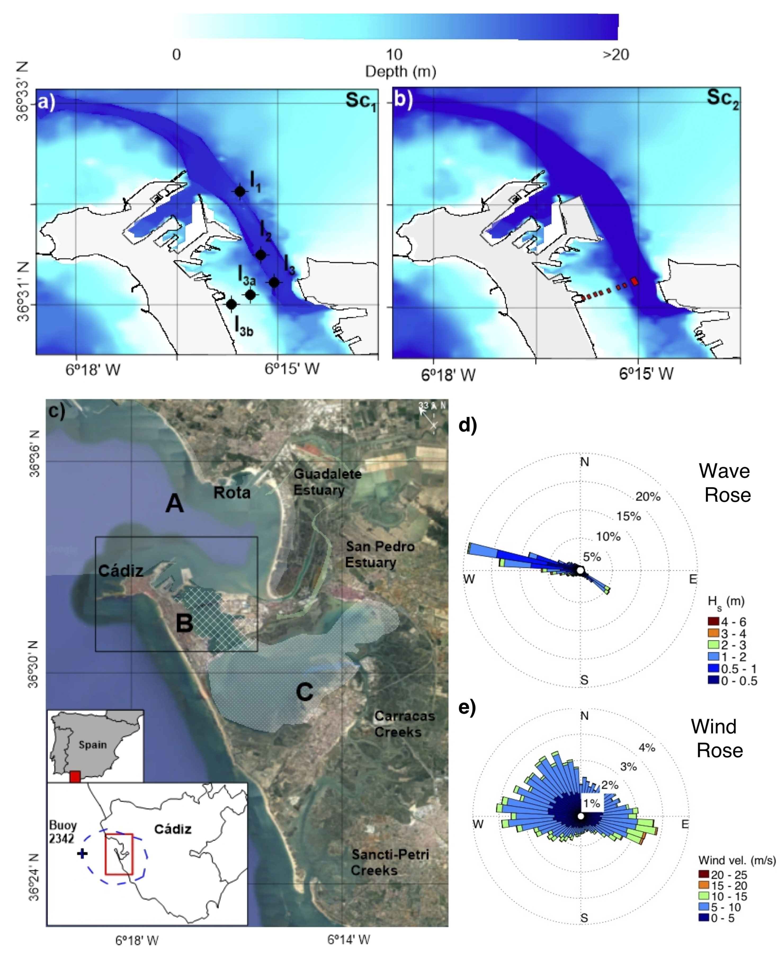
2. Study Site

The Cádiz Bay, located in southwestern Spain (36${}^{\circ }$23${}^{\prime }$–36${}^{\circ }$37${}^{\prime }$N, 6 ${}^{\circ }$12${}^{\prime }$–6${}^{\circ }$20${}^{\prime }$W, Figure 1c) has a total area of 7000 ha and is formed by five well-defined areas: (1) the outer bay (A in Figure 1c), with 70 km${}^2$ and an average depth of 15 m, (2) the Puntales Channel (PC, B in Figure 1c), a 3.8 km-long and 1.3 km-width constriction with maximum depths of 18 m, (3) the inner bay (C in Figure 1c), a 50 km${}^2$ basin characterized by gentler slopes, shallower depths (between 0.5 and 8 m) and the presence of a multitude of low-lying mudflats cut by deeper tidal channels, and (4) and (5) two tidal creek systems (Carracas and Sancti-Petri, Figure 1c), which constitute a second connection of the inner bay with the open sea. In recent years, different human interventions have been developed in areas A and B to increase the capacity of the Port of Cádiz Bay. In particular, a new terminal has been built, which will involve in the future the deepening of the navigation channel that gives access to it, as well as a new bridge that crosses the Canal de Puntales and for which 7 piers have been built that can alter the local hydrodynamics (Figure 1a,b [12]).

The main forcings governing the estuary dynamics are tides, wind and waves. The bay is a mesotidal estuary with tidal ranges varying between 2 and 4 m. The tide is predominantly semidiurnal, with the M2 being the most energetic constituent. The interaction between M2 and other semi- and quarter-diurnal constituents generates monthly and fortnightly variations in hydrodynamics, with maximum flow velocities over 1.5 m/s. The dominant winds in the Cádiz Bay (data from buoy 2342, Figure 1c, Puertos del Estado, Ministerio de Transportes, Movilidad y Agenda Urbana, Spain) have an important seasonal variability, with strong winds from the N-W sector predominantly between January and April, and moderate winds between July and September (Figure 1e). The most energetic winds come generally from the SE. The predominant swell comes from the W-SW sector, with average significant wave heights of around 1 m and storms with wave heights above 3.8 m (Figure 1d).

The temperature and salinity regime within the bay has an important seasonal variation compared to open waters, being generally hypersaline in winter and hyposaline in summer. Salinity values vary between 37 and 34 psu, and the temperature ranges between 10 and 35 °C, with minimums and maximums in winter and summer respectively [28]. The highest salinity variation with respect to the ocean occurs in PC, mainly due to the high evaporation rates (1320 mm/year) and the low amount of annual rainfall (600 mm/year) in the study area.

3. Methodology

3.1. Numerical Model

3.1.1. Model Description

In this study, the Delft3D model, developed by WL|Delft Hydraulics, was used in its depth averaged (2D) configuration. This model solves the shallow water equations with Boussinesq and hydrostatic approximations [29]. The continuity equation, assuming incompressible flow, is described by:

$${\displaystyle \frac{\partial u}{\partial x}}+{\displaystyle \frac{\partial v}{\partial y}}=Q$$

(1)

where Q represents the transport of mass per unit area and u and v are the velocity components in the directions x and y, respectively.

The momentum equations are defined as:

$${\displaystyle \frac{Du}{Dt}}=-{\displaystyle \frac{1}{{\rho }_0}}{P}_x+F_x+M_x+fv$$

(2)

and:

$${\displaystyle \frac{Dv}{Dt}}=-{\displaystyle \frac{1}{{\rho }_0}}{P}_y+F_y+M_y+fu$$

(3)

where g is the acceleration due to gravity, t is time, ${\rho }_0$ is the reference density of water, f is the Coriolis parameter, $P_x$ and $P_y$ are the horizontal pressure gradients for both directions, including the terms due to baroclinic gradients, $F_x$ and $F_y$ represent Reynolds’ horizontal tensors in the x and y directions, respectively, and $M_x$ and $M_y$ represent contributions due to external sources or sinks of momentum, such as wind action on the water surface or wave action in the water column.

The transport equation used to model salinity and temperature is the advection-diffusion equation:

$${\displaystyle \frac{Dc}{Dt}}={\displaystyle \frac{\partial }{\partial x}}\left(D_h{\displaystyle \frac{\partial c}{\partial x}}\right)+{\displaystyle \frac{\partial }{\partial y}}\left(D_h{\displaystyle \frac{\partial c}{\partial y}}\right)+S_c$$

(4)

where c is the concentration, $D_h$ is the horizontal diffusivity and $S_c$ represents the source/sink terms per unit area. For depth averaged simulations, $D_h$ is obtained as the combination of the diffusion due to the sub-grid scale turbulence and a user-defined horizontal diffusion coefficient accounting for all other forms of unresolved mixing that is used as a calibration parameter. Both the hydrodynamic and transport equations are solved by finite differences in a structured curvilinear grid.

Wave propagation processes are modeled using a Delft3D module based on SWAN, a third generation spectral wave model [30] that considers processes such as shoaling, refraction, diffraction, wind generation and wave-current interactions, among others, through the wave action conservation equation. For energy dissipation, the model considers depth-induced wave breaking, bottom friction and whitecapping. This module is coupled online with the hydrodynamic and transport module by including the force exerted by the waves in Equations (2) and (3), while the water levels and currents of the hydrodynamic module are considered for the wave propagation.

3.1.2. Model Setup

The domain of the model was defined by a curvilinear computational grid (Figure 1c), with a total of 365 × 245 cells and a maximum resolution of 20 × 20 m${}^2$ in the area of Carracas and Sancti-Petri creeks. The initial condition for the simulations was water at rest (cold start) and salinity and temperature values of 15${}^{\circ }$ and 36.5 psu, respectively. After different tests with the model, the simulated period used for the model spin-up was one month after a trial–error process [31,32,33], after which the results to be analyzed were obtained.

The average river discharge values of the Guadalete and San Pedro rivers were introduced as discharges due to their low inflow rates, while at the open boundaries a water level condition was used considering the eighteen main constituents of the astronomical tide, i.e., M2, S2, SA, Q1, O1, P1, K1, 2N2, MU2, N2, NU2, L2, T2, R2, K2, MN4, M4 and MS4, obtained using the Oregon State Tidal Prediction model [34]. Wind and wave forcings with 3-h intervals obtained from the Buoy 2342 were introduced in the whole domain and the boundaries, respectively. To calculate heat transport (at regional scale), daily data on solar radiation, temperature, atmospheric humidity and cloudiness were obtained from the Andalusian regional government. The data are available in Zarzuelo et al. [35].

3.1.3. Model Calibration and Testing

The model was calibrated and tested for the following variables: water levels, east and north velocities, salinity and temperature using field data obtained from Acoustic Doppler Current Profilers (ADCP) and Conductivity Temperature (CT) instruments deployed simultaneously at the locations shown in Figure 1a. In previous studies [12], a similar model implementation was calibrated and tested for hydrodynamics, although for the present work the grid resolution at the creeks was increased to properly capture this connection to open sea. Hence, the validation process was repeated, including also the salinity and temperature variables. The calibration period was from 4 January–22 January 2012 (I1-I3, Figure 1a), where the first field campaign took place. The data measured in the second field survey (24 May–10 June 2013; I3-I3a-I3b, Figure 1) were chosen for testing. The hydrodynamic values of I2 could not be used due to deployment issues with the ADCP. The agreements are excellent for sea level and velocities (R${}^2$≈ 0.99 and ≈ 0.89, respectively) and good for salinity and temperature (R${}^2$≈ 0.80 and ≈ 0.78, respectively) both for the calibration and testing periods (see supplementary material for further details).

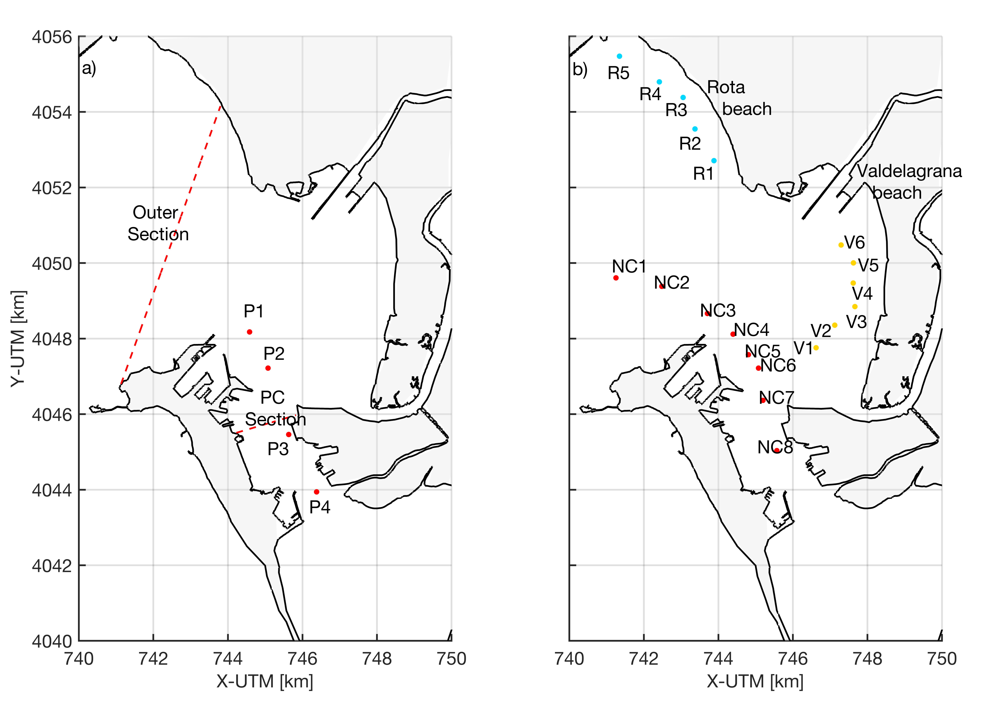
3.2. Modeled Scenarios and Locations of Interest

The simulation period runs from October 2012 to November 2013. This period of approximately one year is characterized by an average significant wave height of 1.5 m, reaching maximum values in winter (H${}_s$≈ 5 m) coming from the NW (Figure 2a,b). Winds come usually from the NW-SW and NE-SE with average speeds of 6 m/s (Figure 2c). Storms are more frequent in winter with wind speeds up to 15 m/s. The river discharges are reduced (10 m${}^3$/s and 30 m${}^3$/s for the San Pedro and Guadalete rivers, respectively), considering the tidal prism of the bay (4 × 10${}^5$ m${}^3$, [36]). This year can be considered representative year due to these forcing; it is also selected due to its proximity to the date of the bathymetric data.

The outer bay and PC have undergone modifications since 2017 due to the construction of the new terminal (Figure 1b), which will require the displacement of the navigation channel to the east with the consequent change of its geometry and depth, and the new bridge whose piers have been designed crossing the PC constriction. The new terminal has a length of 590 m, an area of 3.8 km${}^2$ and a maximum depth of 16 m. To achieve the maximum depth of 20 m in the new section of the navigation channel, a dredging of 3.86 × 10${}^6$ m${}^3$ will be performed. The bridge built over PC has been designed with a length of 5 km and a height of 69 m above sea level. These interventions, concentrated on the area close to the connection between the outer bay and PC, were included in the bathymetric scenario Sc${}_2$ (Figure 1b), while Sc${}_1$ (Figure 1a) maintains the pre-intervention bathymetry.

Considering the areas in which Zarzuelo et al. [12] identified changes in the tidal harmonics characteristics for these interventions, four points have been selected for the analysis of the results in terms of tidal wave, waves and morphodynamic implications. In addition, two sections have been defined to analyze the exchange of water and salt between the ocean and the outer bay, and the outer bay and PC due to baroclinic, barotropic and wind related effects (P${}_i$, Figure 3a). In these sections, salinity is used as a conservative constituent to calculate changes in water renewal. Finally, 20 points (Figure 3b) distributed along the navigation channel at the entrance to PC and two beaches in the outer bay (Valdelagrana and Rota) have been used to analyze whether the interventions may cause changes in the morphodynamics of these beaches due to changes in the magnitude or direction of wave energy flux. The definition of the locations of these points, as well as their number and separation, was made after an analysis of the model outputs considering the spatial scale of the variability of the different variables, ensuring the representativeness of the obtained results.

3.3. Variables Analyzed

3.3.1. Water and Salt Exchange in the Bay

The flushing time of a water body is defined as the time required to replace the water inside the body through a given section. This determines the time scale of water transport through that section and, therefore, the time available for the renewal rate of conservative constituents, such as salt. The flushing time is obtained as:

$$T_f={\displaystyle \frac{V}{Q}}$$

(5)

where V is the volume of the water body and Q is the instantaneous rate of water transport in the study section [37,38] that connects the water body to the outside. This flushing time is analyzed in both sections of Figure 3a in order to understand how the ocean-outer bay and outer bay-PC water renewal rates are modified as a consequence of the interventions.

Chen et al. [23] analyzed the water and salt transport from another perspective, defining the residual water unit width flux ($R_w$) and the residual unit width salt flux ($R_s$) as:

$$\overrightarrow{R_w}={\displaystyle \frac{1}{T}}\int \overrightarrow{q}dt$$

(6)

and:

$$\overrightarrow{R_s}={\displaystyle \frac{1}{T}}\int \overrightarrow{q}Sdt$$

(7)

where the arrow indicates vector variables, t is time, T is the average time scale, which in this case is equal to the dominant tide cycle (12.45 h), S is salinity and $\overrightarrow{q}$ is the instantaneous rate of water transport per unit width through a water column:

$$\overrightarrow{q}={\int }_{h_1}^{h_2}\overrightarrow{v}dz$$

(8)

with $\overrightarrow{v}$ being the flow rate, $h_1$ and $h_2$ the depths for the surface and bottom layers, and z the total depth.

The analysis of these variables was carried out on the period with the highest currents (spring tides for all the simulated fortnightly periods) where the greatest baroclinic changes are generated, and therefore where the greatest residual flows will occur. For neap tides, residual flows are lower and even negligible [28]. The variables defined above allow for the analysis and interpretation of the modifications that occur in the transport of salt due to the interventions, as will be shown in Section 4.2.

Regarding the salt transport, variations in salinity (S) in the outer bay are triggered only by salt transport through PC, except in summer when evaporation is important. Variations in salt transport through PC drive an exchange rate (R) defined as [24]:

$${\displaystyle \frac{\partial S}{\partial t}}{|}_{\mathrm{exchange}}=R\Delta S$$

(9)

where $\Delta S=S_i-S_0$ is the average difference in salinity between the PC (S${}_i$) and the outer bay (S${}_0$), and $\partial S/\partial t$ is the variation in salinity of the outer bay over a certain period of time. Thus, the greater $\Delta S$, the faster the salinity gradient decreases. This exchange rate R depends on several processes such as wind-driven, barotropic and baroclinic flows, and the contribution of each of these processes to R can be obtained separately providing a proxy of how interventions in the bay modify the transport of salt between basins.

The contribution due to barotropic flows ($R_{\mathrm{tide}}$) is induced by the astronomical tide as [24]:

$$R_{\mathrm{tide}}={\displaystyle \frac{\mu }{t_{\mathrm{tide}}}}{\displaystyle \frac{V_{\mathrm{prism}}}{V}}$$

(10)

where $V_{\mathrm{prism}}$ and V are the tidal prism and the water volume of the outer bay, $t_{\mathrm{tide}}$ is the dominant period of the tide and $\mu$ is the retention coefficient, defined as $\mu =(\delta S_{\mathrm{tide}}/\Delta S)(V/V_{\mathrm{prism}})$ where $\delta S_{\mathrm{tide}}$ is the variation of salinity for a tidal cycle at the outer bay.

The baroclinic exchange is related to the effects that variations in water density have on the flow through the exchange sections. According to Hearn and Robson [24], the baroclinic exchange rate ($R_{\mathrm{baroclinic}}$) can be calculated as:

$$R_{\mathrm{baroclinic}}={\displaystyle \frac{A\sqrt{(\Delta \rho /\rho )g{h}_{\mathrm{PC}}}}{4V}}$$

(11)

where A and $h_{\mathrm{PC}}$ are the minimum section and the average depth of PC, respectively, and $\Delta \rho$ the difference in density between the two basins analyzed.

The exchange rate triggered by wind ($R_{\mathrm{wind}}$) is defined as [39]:

$$R_{\mathrm{wind}}={\displaystyle \frac{\mu }{t_{\mathrm{wind}}}}{\displaystyle \frac{V_{\mathrm{wind}}}{V}}$$

(12)

where $V_{\mathrm{wind}}$ is the water volume variation due to wind and $t_{\mathrm{wind}}$ is the dominant period of the wind changes, for which 3 h were considered after analysis of the wind data. The changes in water elevation ($\Delta \eta$) cause $V_{\mathrm{wind}}$, being that variation equal to $(V\Delta \eta )/\left(2h_{\mathrm{basin}}\right)$ where $\Delta \eta =(\beta C_W{\rho }_{\mathrm{air}}L\left|W\right|W)/\left(\rho g{h}_{\mathrm{basin}}\right)$, being $\beta$ a friction coefficient (0.8, [40]), ${\rho }_{\mathrm{air}}$ the air density (1225 kg/m${}^3$), $C_W$ the wind drag coefficient (0.005, obtained after model calibration), L the length of the basin measured over the navigation channel, $h_{\mathrm{basin}}$ the mean depth of the basin, $\rho$ the mean water density and W the wind speed.

Finally, to determine the value of relative hypersalinity as a simple salt balance between the outer bay and PC, the net exchange rate defined in Equation (9) is balanced by the evaporation rate E [24,41]. Therefore, salt exchange is defined as:

$$R_{\mathrm{hyper}}={\displaystyle \frac{\Delta S}{S_i\ast (E/h_{\mathrm{basin}})}}$$

(13)

3.3.2. Influence of Waves

For the analysis of the influence of waves, the yearly-average wave energy flux per crest $\overline{F}$ width has been used, whose module for each sea state is defined as:

$$F={\displaystyle \frac{1}{8}}\rho g{H}^2{c}_g={\displaystyle \frac{1}{8}}\rho g{H}^2{\displaystyle \frac{c}{2}}\left(1+{\displaystyle \frac{2kh}{sinh\left(2kh\right)}}\right)$$

(14)

where H is the significant wave height, $c_g$ is the group celerity, c is the wave celerity, k is the wave number and h is the water depth. This energy flux, which has the direction of the waves, was obtained for each sea state propagated during the simulations carried out, and its annual average was obtained for the pre- and post-intervention scenarios. With the results, two possible impacts on the bay were analyzed: (1) the effect on the navigation channel to study how the planned dredging can affect the navigability conditions (NC${}_i$, Figure 3b); and (2) the impacts on the coastal dynamics of the beaches in the outer bay (R${}_i$ and V${}_i$, Figure 3b), since variations in magnitude and direction of the yearly average wave energy flux can cause the rotation of their shorelines [42].

4. Results and Discussion

Previous studies analyzed the effects of the interventions on the hydrodynamic and morphodynamic behavior of Cádiz Bay [12,26]. However, these studies only considered tidal and wind forcings, neglecting the effects of waves and baroclinic flows, even when they may cause variations in the behavior of the outer bay and its connection with PC. Moreover, these works considered simulations of 2-month duration, preventing the analysis of the seasonal variability which plays a major role on the baroclinic processes. In contrast, the results presented and discussed throughout the next paragraphs include all these processes, being of interest for researchers analyzing other coastal environments where only short-term simulations are used [43,44].

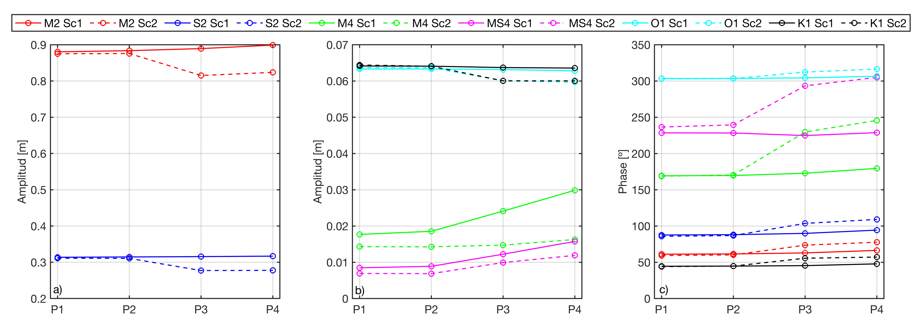
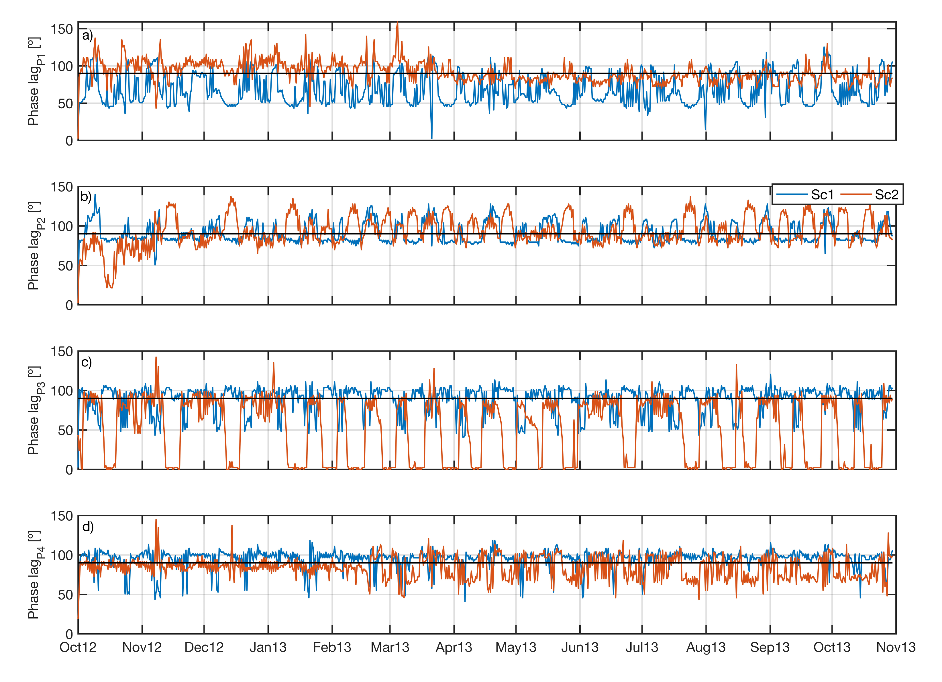
4.1. Tidal Dynamics

In this section, the tidal dynamics at P${}_i$ (Figure 3a) are analyzed. The results obtained for the amplitude and phases of the main tidal harmonics are shown in Figure 4. For Sc${}_1$ the main changes as the tidal wave propagates towards PC are the increase of the amplitudes of M2 (8%) and of the quarter-diurnal overtides M4 and MS4 (18%), while the phases remain relatively constant. This increase in the quarter-diurnal components implies that, before the interventions, friction, advective processes and sediment transport increased along PC. The M2 takes 12.45 min to travel from P1 to P4, 10 km apart (wave speed c${}_{\mathrm{M}2}$ = 13.39 m/s). If compared with the wave speed in shallow areas c${}_0=\sqrt{gh}$, a similar speed is obtained (11.5 m/s) and therefore the bay could be considered a convergent system [45,46,47].

However, if compared to the results for Sc${}_2$, it is observed that for all tidal harmonics the amplitude decreases at all points, but especially in the inner PC (points 3 and 4). The decrease (30%) in the quarter-diurnal harmonics implies that the effect of friction is reduced after the interventions, and therefore non-linearities, transport and mixing processes are consequently reduced. As for the semi-diurnal components, they decrease up to 10%, so the effect of flow constriction that was observed before the interventions and caused an increase in the current velocities [12] is clearly limited by the interventions. In addition, the phases also increase, decreasing the wave celerity with 27 min delay triggered by a greater tidal prism. Comparing the speed of the tidal wave M2 (c${}_{\mathrm{M}2}$ = 4.36 m/s) with the shallow water wave celerity (c${}_0$ = 11.18 m/s), it can be concluded that PC is evolving to a damping system after interventions. This behavior can be of interest to reduce the effects of sea level rise due to climate change [48]. For the diurnal harmonics, a decrease in amplitude of about 10% is observed after the interventions, while the phases increase in the same way as the semi-diurnal harmonics.

These results contrast to those obtained by Zarzuelo et al. [12,26]. Although the behavior of M2 is similar, the diurnal components undergo significant changes that can be attributed to the inclusion of waves and baroclinic flows. The decrease of the amplitudes of the quarter-diurnal harmonics not observed previously, although the increase in tidal asymmetry (a${}_{\mathrm{M}4}$/a${}_{\mathrm{M}2}$) from 0.009 (Sc${}_1$) to 0.019 (Sc${}_2$) up to P3 and the reduction from P3 to P4 (from 0.01 to 0.007), resulting in increased sediment transport, was already described by Zarzuelo et al. [26].

To further analyze the effect on the tidal dynamics, the phase lag between high water and high water slack was obtained to identify changes in the tidal wave type [49,50]. For phase lags close to 90${}^{\circ }$, the tidal wave is stationary and the high water is reached throughout the basin simultaneously, which is characteristic of semi-closed water bodies acting as reservoirs. For lags close to 0${}^{\circ }$, the wave is purely progressive, characteristic of frictionless channel of constant cross-section and infinite length [45]. Figure 5 shows the results obtained; for Sc${}_1$ the phase lag (${\varphi }_{a_{M2}}-{\varphi }_{u_{M2}}$) is close to 90${}^{\circ }$ for points P2, P3 and P4, indicating that the tidal wave is quasi-stationary. At neap tides they become mixed due to the involvement of the overtidal components (M4 and MS4), this difference being more relevant at the points inside PC (P3 and P4). This periodicity has implications in the increase of the bed shear stresses, and therefore in the sediment transport, contributing to the increase of the tidal asymmetry dominated by flood tides on the shallower areas [51]. These observations are in agreement with Zarzuelo et al. [26], where the dominance of flood tides (2${\varphi }_{\mathrm{M}2}-{\varphi }_{\mathrm{M}4}$) was analyzed after the interventions. However, in P1 (Figure 5a), during most of the year tidal wave is mixed (<${90}^{\circ }$), being stationary only for high water at spring tides. Therefore, before the interventions the inner part of the PC behaved like a reservoir at high tides. After the interventions, the major changes are observed at P1 and P3 (Figure 5a,c). At P1 the tidal waves becomes quasi-stationary, and at P3 it varies between stationary and progressive depending on spring and neap tides, respectively. This is in agreement with the decreases in amplitudes and increases in tidal phases previously described. Finally, the tidal wave at P2 and P4 (Figure 5b,d) become mixed for most part of the year. These changes will cause a reduction in the tidal asymmetry due to the increase in depth, leading to a possible reduction in sedimentation in this area and an increase in the residual currents.

4.2. Impact on Water Quality and Renewal Time

The spatial distribution of $R_w$ and $R_s$ for spring tides and their variations after the interventions are shown in Figure 6. For Sc1 (Figure 6a), $R_w$ is directed towards open water through the navigation channel. However, on the sides of the channel and in the inner bay it flows in the opposite direction. This is due to tidal pumping and the Stokes drift [52], being the inner bay renewed with water from the ocean. The lowest values ($\approx 0.01$ m${}^3/$s) are found in the shallow areas due to the effect of friction, while the highest values ($\approx 0.1$ m${}^3/$s) are obtained in PC due to the flow constriction. Figure 6b shows the distribution of $R_s$, being very similar to that of $R_w$. Due to higher salinity concentrations in the ocean and along the navigation channel in the outer bay and PC, the baroclinic influence is greater in these areas.

The differences in the $R_w$ and $R_s$ distributions between scenarios are shown in Figure 6c,d, respectively. The largest differences in both (15%) occur around the navigation channel, where either the water depth and the geometry of the section have changed. In addition, the baroclinic effect is larger (7%) in the outer bay because of its greater differences in salinity (10%). The directional changes show two trends: (1) in the outer bay, where the vectors rotate slightly counterclockwise and (2) in PC, where vectors rotate towards the channel margins, which will cause an increase of the sedimentation in the shallower areas of PC. There is no difference between the directions of R${}_w$ and R${}_s$ after the interventions. Therefore, it can be concluded that the interventions intensify the importance of the baroclinic effects, due to the increase in the difference in salinity between the outer bay and PC as a consequence of the increase of the water volume in which salt have to be dissolved.

Figure 7 shows the percentage of time in the simulated year during which the flushing time in a tidal cycle exceeds a certain number of days for the two defined sections. It is observed that for Sc${}_1$ the flushing time is 15–20 days for the outer bay (Figure 7a), exceeding 50 days during some tidal cycles, especially during summer and winter storm periods. In the case of PC, the average is 5 days with fortnightly variations due to spring/neap cycles (Figure 7b), rarely exceeding 50 days in summer. The changes triggered by the interventions (Sc${}_2$, orange line Figure 7c,d) are much more evident for PC, increasing the probability of exceeding 10 days by 40%, which implies that there is a greater renewal of water from PC. In the outer bay the values are very similar with a slight variation with respect to Sc${}_1$ (5%), increasing the probability of occurrence for 0–40 days, and decreasing for 60–80 days.

The average of the total exchange rate R between the outer bay and PC was calculated for Sc${}_1$ using Equation (9), resulting in a value of 1.9 days. On the other hand, the barotropic, baroclinic, wind and hypersalinity contributions to R were obtained (Figure 8) in order to find out which process dominates the salt transport. For this section, the data defined in the

Table 1. Values used in the calculation of exchange rates.

Parameter	Data
$A_{\mathrm{PC}}$	4.94 × 10${}^6$ m${}^2$
$\Delta \rho /\rho$	9.8 × 10${}^{-4}$
$h_{\mathrm{PC}}$	10 m
$\Delta \eta$	0.017 m
$h_{\mathrm{basin}}$	10 m
L	10000 m
V	8.19 × 10${}^8$ m${}^3$
$V_{\mathrm{prism}}$	1.19 × 10${}^8$ m${}^3$
$V_{\mathrm{wind}}$	1.43 × 10${}^6$ m${}^3$

were used. The average value of $R_{\mathrm{tide}}$ is 1.20 days, with a high variability associated with spring/neap tidal cycles. The average values obtained for $R_{\mathrm{baroclinic}}$ and $R_{\mathrm{wind}}$ are 24.4 and 0.03 days, respectively. Finally, $R_{\mathrm{hyp}}$ is equal to 0.05 days throughout the year except in summer when it increases to an average of 0.5 days, reflecting the importance of evaporation in salt transport in that period. Subtracting $R_{\mathrm{wind}}$ and $R_{\mathrm{hyp}}$ from R yields a value of ≈ 1.32 days, which is very similar to that of $R_{\mathrm{tide}}$. Therefore, if periods of high evaporation and intense winds are not considered, it can be concluded that salt exchange is controlled by the tide, the baroclinic term being negligible.

For the post-intervention scenario, the value of R calculated with Equation (9) (Figure 8e) shows an important increase (15%) during storm eventos in winter resulting in a slower mixing, and therefore a longer time of salt renewal. For the rest of the year, R is reduced (2%), causing a slight acceleration of the salt exchange process. If the barotropic, baroclinic, wind and hypersalinity processes are analyzed, the results show that $R_{\mathrm{tide}}$ (Figure 8a) and $R_{\mathrm{wind}}$ (Figure 8c) are not influenced by the development of the interventions. However, $R_{\mathrm{baroclinic}}$ (Figure 8b) shows a slight decrease (10 %) in summer and an increase of 20 % in winter. On the other hand, $R_{\mathrm{hyp}}$ (Figure 8d) is reduced by almost 20%, reaching the maximum differences in winter and summer (50%). Therefore, after the deepening of the navigation channel, the influence of the tide and wind is negligible, while the baroclinic processes accelerate the mixing process in the bay during almost the whole year.

4.3. Changes in Salinity and Temperature

Figure 9 represents the annual distribution of temperature and salinity for the 4 locations defined. For Sc${}_1$ the salinity decreases from P1 to P3 (from 36.3 to 36 psu, Figure 9f) and then increases towards P4 (36.2 psu, Figure 9h). The lowest values are those found in March-April due to increased precipitation, while the highest values are reached in July-August due to high evaporation. The temperature follows the same trend as the air temperature, which in turn shows clearly a seasonal variability. It is observed that values are very similar at all points, being slightly lower at P3 and P4 (Figure 9e,g, respectively; 1–2${}^{\circ }$). See Zarzuelo et al. [28] for further details.

After interventions (Figure 9), all points experience an increase in temperature (1–2${}^{\circ }$; Figure 9a) between the months of October to February, and a decrease of (1–2${}^{\circ }$) for the rest of the year. On the contrary, the salinity (Figure 9b) shows an increase from November to January, highlighting the changes in P3 and P4 (20%; Figure 9e–h). For these points, the temperature drops by 3–4${}^{\circ }$ and the salinity by 0.3–0.4 psu during the months of June to August. Therefore, the interventions drive a damping of the temperature and salinity, reducing the seasonal variability and being these variables more homogeneous along the bay. Hence, the renewal time decreases, maintaining a more constant value of salinity and temperature throughout the bay, as there is an increase in the effective section that improves the mixing. This buffering can be beneficial to soften the effects of global warming and the increase in water temperature in future years, maintaining the existing estuary ecosystem [48].

4.4. Potential Changes in Morphodynamics

According to Zarzuelo et al. [26], the critical bed shear stresses ${\tau }_{\mathrm{cr}}$ for erosion and sedimentation of the Cádiz Bay sediment (a mixture of sand and clay) are 1.2 and 0.8 N/m${}^2$, respectively. Figure 10 shows the spatial distribution of the mean amplitude of the bed shear stresses ($\tau$) for Sc${}_1$ and Sc${}_2$ during a period of high tides (higher values of $\tau$, Figure 10). The results show that the bay is characterized by reduced $\tau$ (0–0.3 N/m${}^2$ for Sc${}_1$) compared to ${\tau }_{\mathrm{cr}}$, although there are higher values in the navigation channel $\tau =1$ N/m${}^2$, with very intense residual currents, and around the City of Cádiz, with values of 1.5–2 N/m${}^2$ due to the joint action of tide and wave, then exceeding ${\tau }_{\mathrm{cr}}$ for erosion. After interventios (Figure 10b), the values of $\tau$ increase, expanding the areas where $\tau >1.2$ N/m${}^2$ and therefore where erosion will predominate. The highest values of $\tau$ for Sc${}_2$ (4 N/m${}^2$) are found in the stretch of the navigation channel along PC, where maximum flow velocities occur due to constriction. Therefore, the channel deepening will cause an increase of erosion in the navigation channel (extending its life span), although it will displace this sediment to the shallower areas and therefore possibly decrease the cross section of the PC, modifying the water renewal and salt exchange characteristics for this section.

To analyze in more detail the effects of the interventions, the time distribution of $\tau$ for the 4 points $P_i$ was analyzed, although to synthesize only the results for P1 and P3 are shown (Figure 11 and Figure 12, respectively). In general, it can be seen that the highest values of $\tau$ occur in winter due to the increase in current velocities induced by storms. In particular, ebb periods result in higher $\tau$ mobilizing mostly the sediment inside the channel. After the interventions, an increase of $\tau$ of 30–40% is observed, these increases being greater for spring tides. P1 (Figure 11) and P3 (Figure 12) show the greatest difference between scenarios due to their differences in velocities and the change from standing to progressive tidal wave. The bed shear stress increase will increase the morphodynamic changes, especially in the dredged area, and will therefore have consequences on its life span. Furthermore, it will cause an increase in turbidity in the area due to the sediment mobilization, and although more detailed studies are needed to assess whether this increase in turbidity can be compensated by the reduction of the renewal time, it could have an impact on the biogeochemical conditions of the area.

4.5. Impacts on Wave Propagation and Impacts on Morphodynamics

The yearly-average wave energy flux $\overline{F}$ has been calculated along the navigation channel (NC), and in the beaches of Rota (R) and Valdelagrana (V) (Figure 13a). In NC $\overline{F}$ values are decreasing towards the interior of the bay, this value being negligible at the last point studied (NC9) due to the fact that the wave energy is almost completely dissipated. The direction of propagation in the first points is perpendicular to Valdelagrana beach (NC1-3), while from NC4 the refraction causes the wave to turn towards the interior of the bay. In Rota $\overline{F}$ is practically perpendicular to the beach, with very similar values in all points showing only a slight difference in R4–5. Finally, on Valdelagrana beach $\overline{F}$ decreases in value from V6 to V1, leaving the $\overline{F}$ to be perpendicular to the coast from V1 to V3 due to the effect of the mouth, although the energy content of the waves here is very low.

Figure 13b,c shows the module and direction variations between the two scenarios. After interventions, a decrease of its module is observed along Valdelagrana beach, especially in the less wave-exposed area of the coastline, where it reaches about 20%. $\overline{F}$ rotates only 1–2${}^{\circ }$ anti-clockwise. Considering these small changes and the fact that the module of $\overline{F}$ decreases more or less uniformly along this beach, interventions are not expected to have consequences on its planform, as it does not favor longitudinal energy gradients. Something very similar occurs in the navigation channel, especially towards the inner bay where the $\tau$ values were higher, due to the drastic change in depth and section. Moreover, in this area the change in direction is more pronounced, reaching 7${}^{\circ }$ in NC7. Therefore, the reduction of $\overline{F}$ caused by a decrease in wave height around the new container terminal will improve its operability with respect to the current situation. Knowing that climate change is latent, and that rising sea levels and more severe storms can cause an increase in wave heights, a possible mitigation alternative would be dredging which could reduce the energy content of the waves in the bay. In Rota, $\overline{F}$ is not influenced by interventions, while the direction of R1 only varies by 1${}^{\circ }$. Therefore, the influence of interventions on coastal morphodynamics is very limited. $\overline{F}$ was calculated for the deep water data of buoy 2342 for all available years to determine the root mean square error (RMSE, black dashed line, Figure 13b,c) to determine at which points the effects of the interventions are greatest (exceeding RMSE). The values of the module are lower than RMSE except in NC9, while the directions do not exceed RMSE $=6^{\circ }$ except in NC6 and NC7, where as described above, the greatest effects due to the interventions are observed.

Figure 14 shows the temporal variations of $\overline{F}$ between scenarios for the points analysed above during the whole simulated year. In Valdelagrana, $\overline{F}$ is reduced throughout the year (30%), with oscillating values in V6. In NC (Figure 14) the variations are more remarkable for NC1-3 and NC9, where there is a decrease in $\overline{F}$ with respect to Sc${}_1$ of up to 80%, originated by average wave heights (2 m) coming from SE-E (Figure 14). In Rota (Figure 14c) these oscillations are only about 10%, caused by the same wave conditions as in NC. Therefore, it can be concluded that interventions cause a reduction in the energy content of the beaches of Valdelagrana and Rota, altering the energy that the sediment mobilizes and causing an alteration in its morphodynamics (more relevant in Valdelagrana) for specific events, although the average energy flow for the whole year does not show great differences.

5. Conclusions

In this work, the influence of the deepening of the navigation channel, the construction of a new terminal and a bridge on the renewal rates, salinity and temperature distributions, wave propagation and morphodynamics of a complex bay (Cádiz, Spain) was analyzed. Both the methodology used, based on the implementation of a calibrated and tested numerical model, and the results obtained can be applied to other bays or estuaries where this type of interventions are carried out, in particular for those systems formed by several basins with different characteristics. After the analysis of the results, the following conclusions are drawn:

• The inclusion of wave forcing and baroclinic processes in the numerical simulations allows to capture several effects on tidal dynamics that previous studies failed to analyze, such as the decrease in the amplitudes of the diurnal components as well as the amplification of the changes produced in the semi- and quarter-diurnal components. The deepening of the navigation channel will cause a decrease in the tidal wave, which will lead to a decrease in the overtidal components, reducing the effects due to friction. Also, there is a clear decrease in the celerity of the tidal wave (c${}_{\mathrm{M}2}$), distancing its values from celerity in shallow waters (c${}_0$). At the same time, the tidal wave tends to be more progressive in the inner bay, which is more similar to channels with a constant section and infinite length. This shows how the bay ceases acting as a convergent system to become a damping system, which can potentially soften the effects produced by the projected sea level rise.
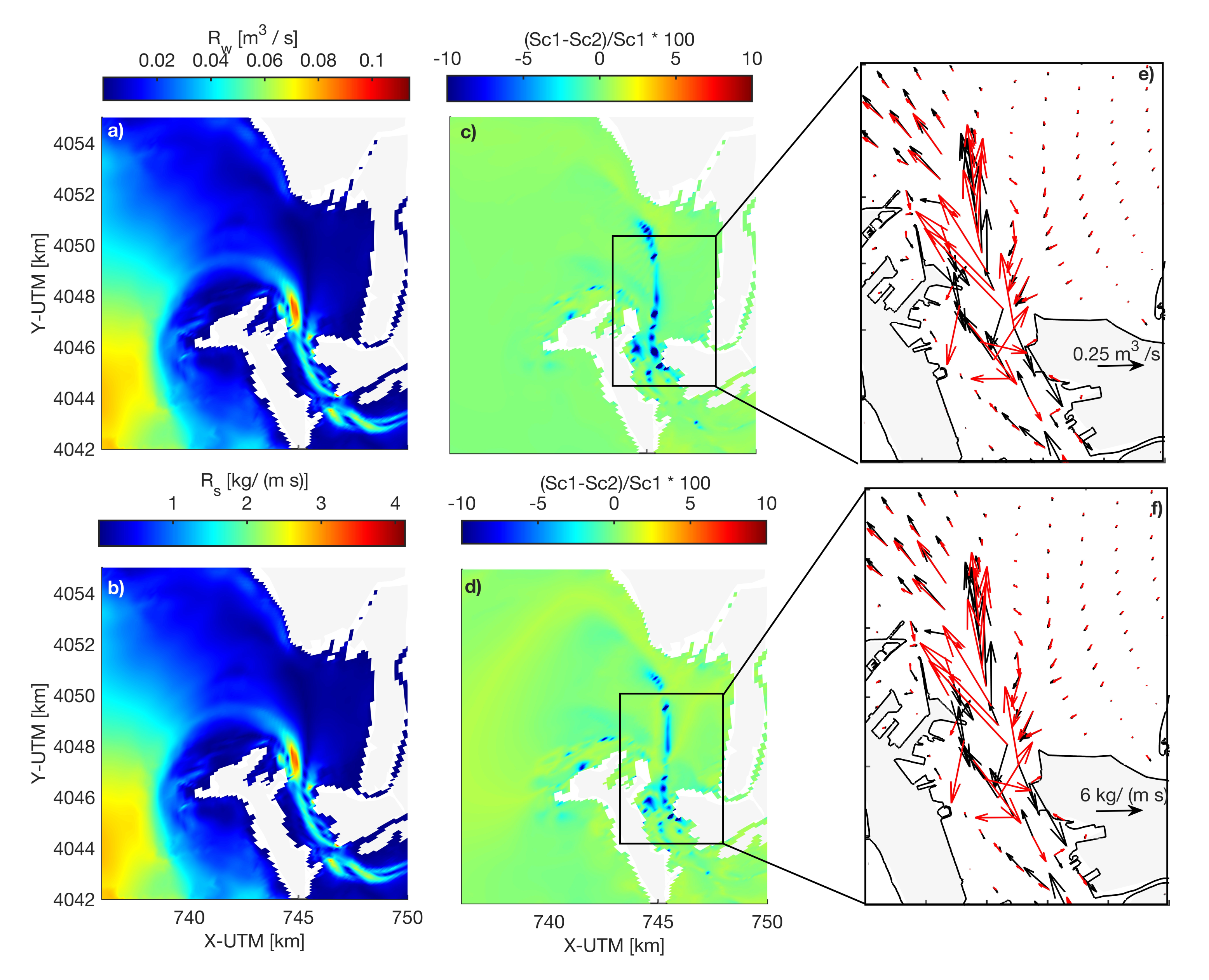
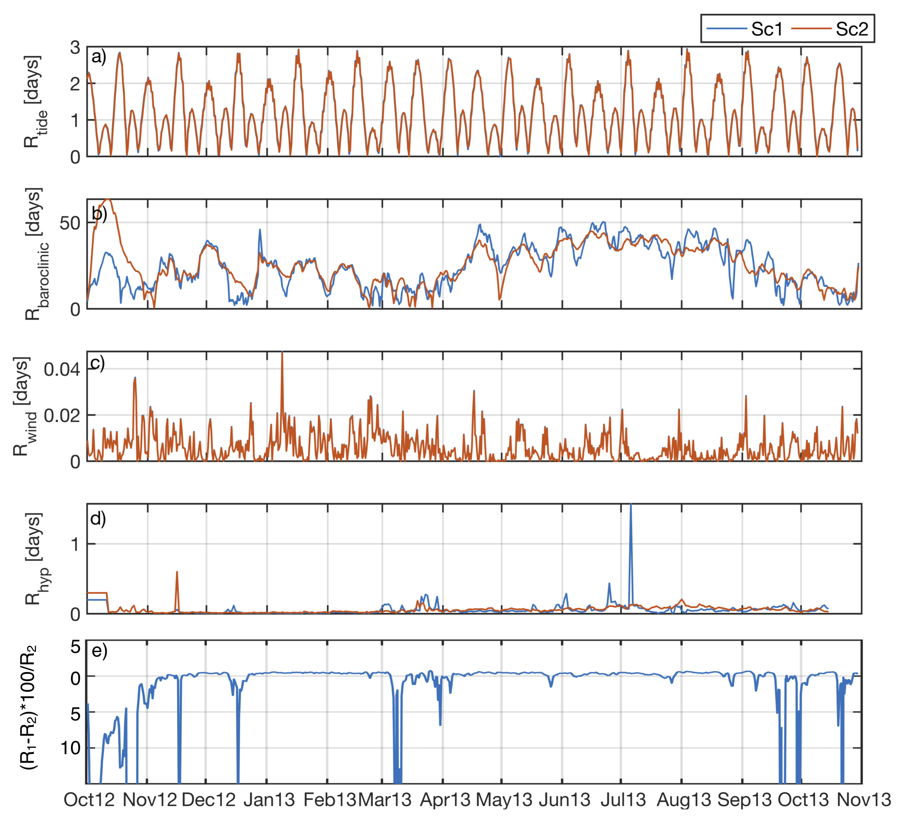
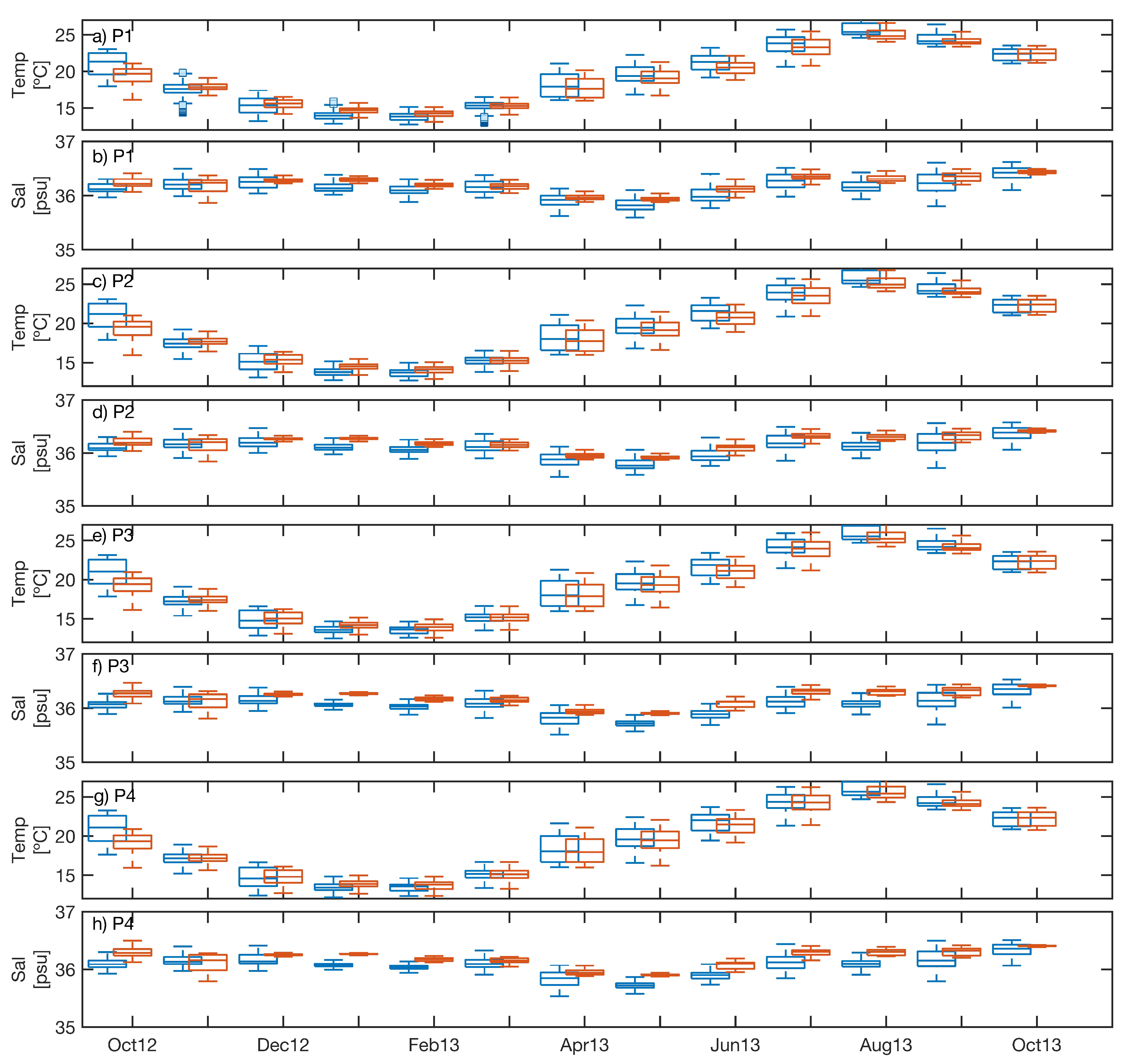
• The greatest changes in salinity and temperature are observed close to the deepening area. R${}_w$ and R${}_s$ are directed towards the margins of the PC, which can change the sediment transport pattern. In addition, dredging intensifies the importance of the baroclinic terms, as the water column increases. The flushing time increases in PC due to the increase of water volume that requires more time for its displacement. These effects can also be observed in the exchange rates where, as the latter increases and as neither R${}_{\mathrm{tide}}$ nor R${}_{\mathrm{wind}}$ varies, R${}_{\mathrm{baroclinic}}$ gains importance. A decrease of R${}_{\mathrm{hyp}}$ is observed, possibly caused by the reduction of the difference in salinity between the outer bay and PC. Finally, it is shown how dredging dumps the seasonal variability of salinity and temperature, something to be considered in the future as climate change will cause an increase in water temperature for the study area.
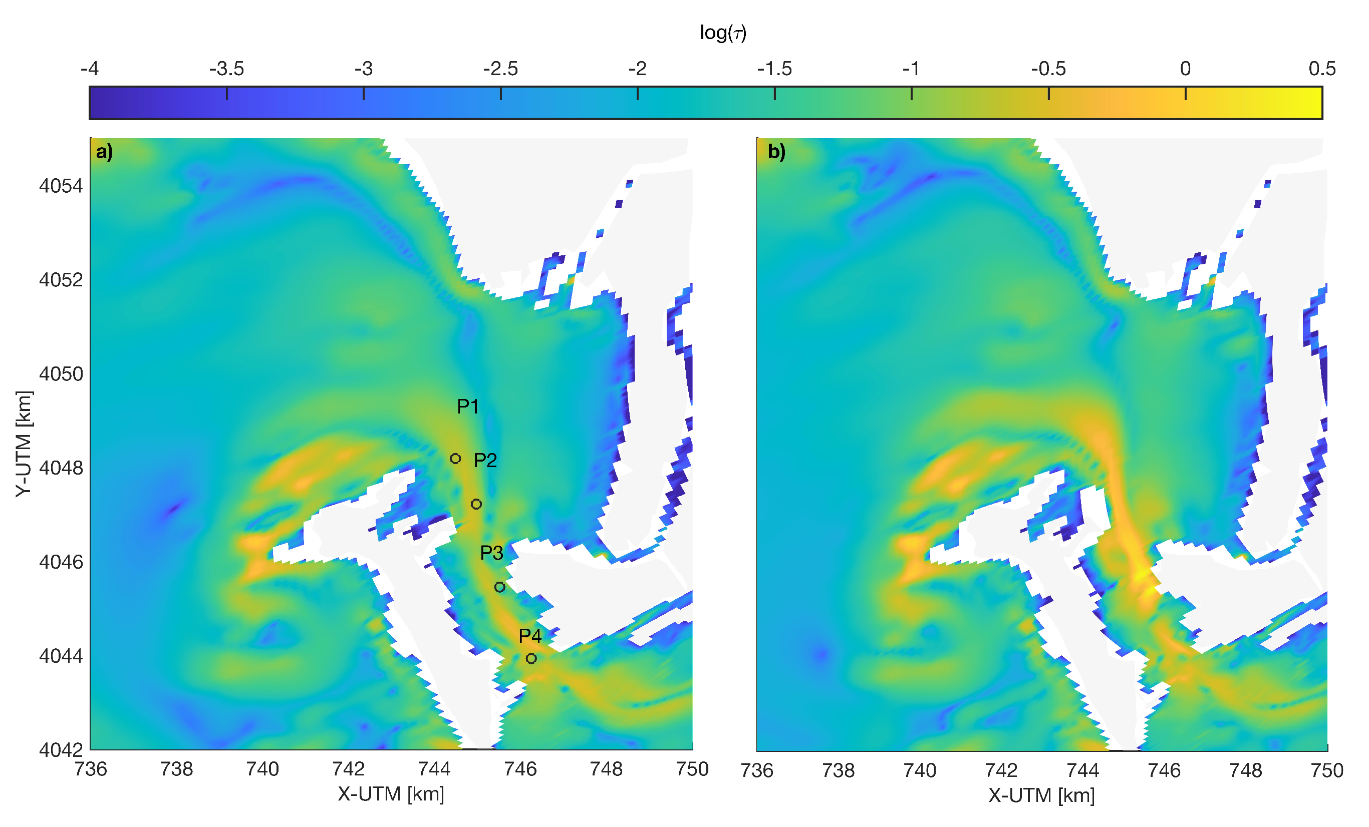
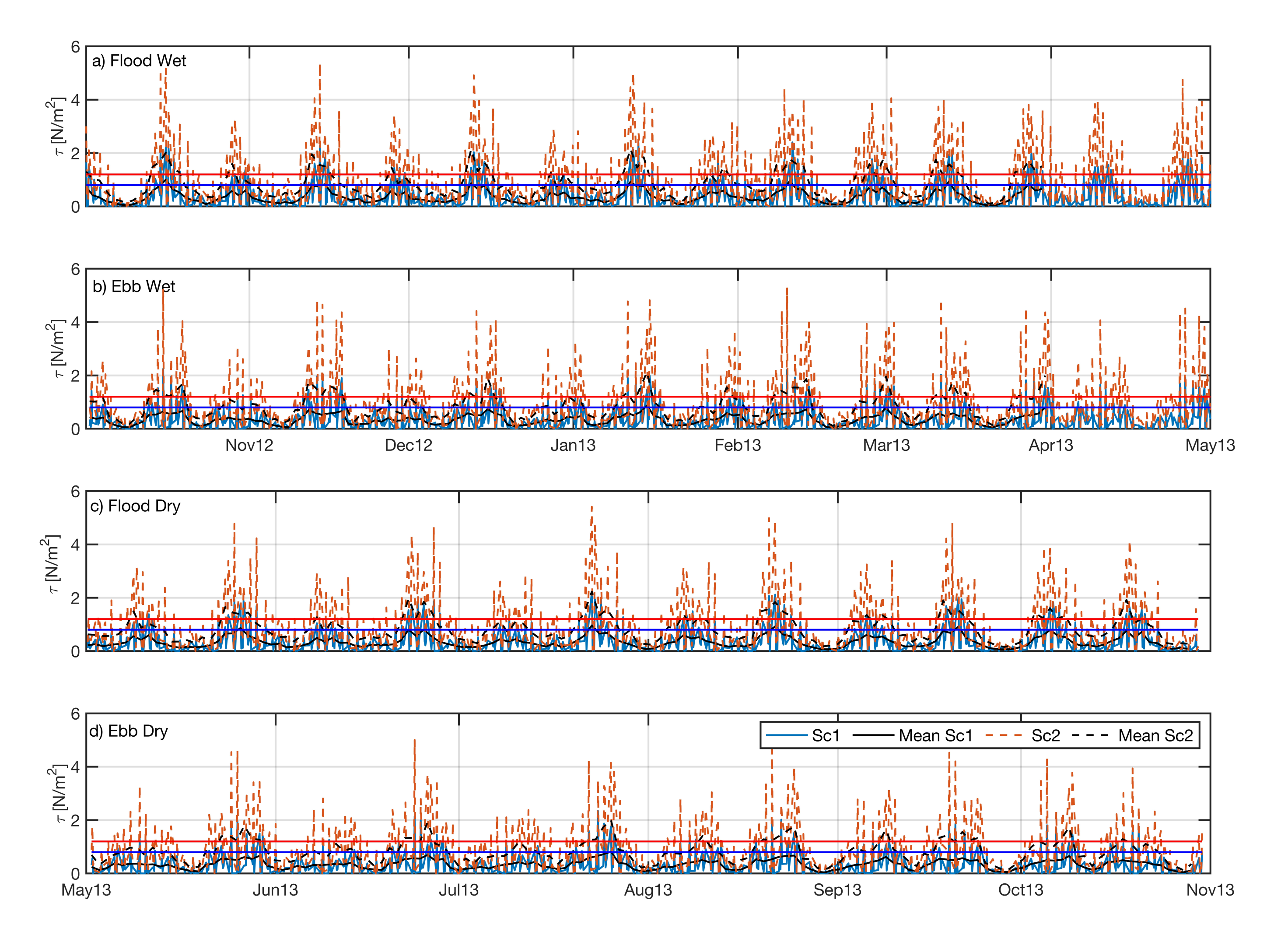
• Regarding the morphodynamics, the deepening of the channel causes an increase in the bed shear stresses, exceeding the critical values of erosion, increasing the lifetime of the dredging but also increasing the sedimentation on its surroundings where the eroded sediment will possibly be deposited, thus decreasing the cross section of PC. Furthermore, such erosion will result in increased turbidity which will impact on the biogeochemistry of PC.
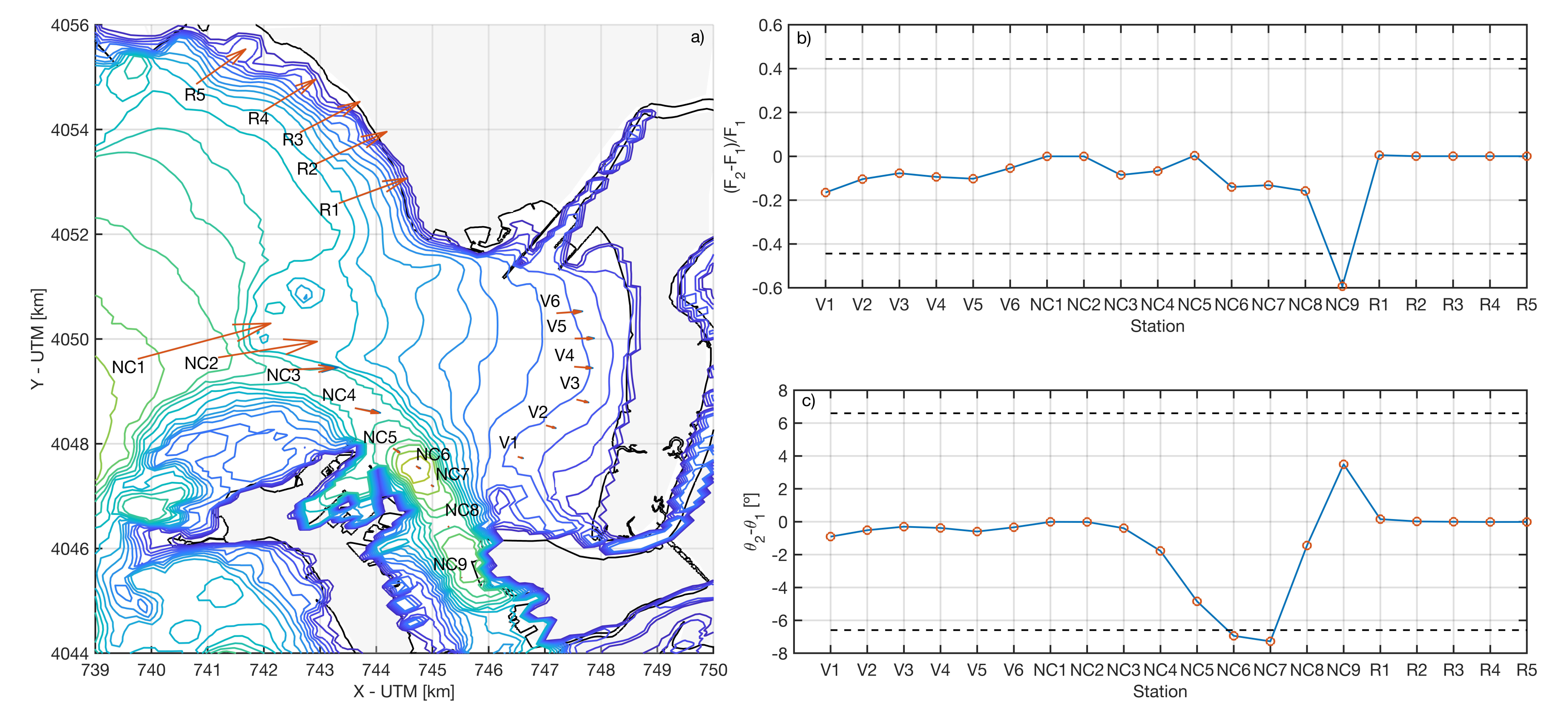
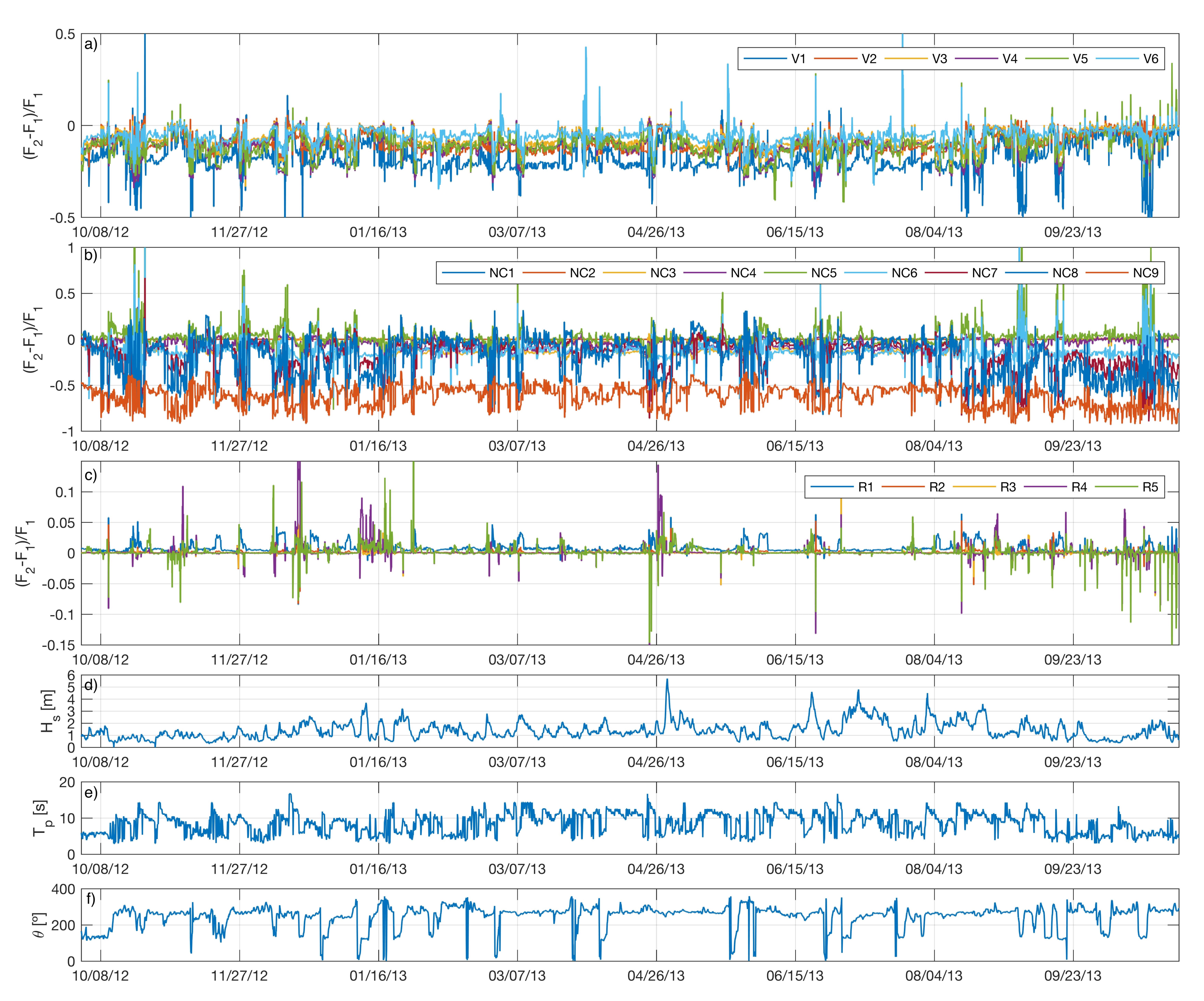
• The greatest changes in wave energy flux are observed in NC, especially near the new terminal where the decrease in wave height due to the channel deepening causes a decrease in the energy flow module, favoring the operation of the new terminal. The changes in the coastal morphology of the beaches of Valdelagrana and Rota will be very limited, although there is a reduction in the energy content that will alter the energy that moves the sediment, especially for certain wave conditions, which added to climate change, can modify the mid- to long-term morphodynamics of these beaches.

References

- Ferrarin, C.; Ghezzo, M.; Umgiesser, G.; Tagliapietra, D.; Camatti, E.; Zaggia, L.; Sarretta, A. Assessing hydrological effects of human interventions on coastal systems: Numerical applications to the Venice Lagoon. Hydrol. Earth Syst. Sci. 2013, 17, 1733–1748. [Google Scholar] [CrossRef]
- French, J.; Burningham, H.; Thornhill, G.; Whitehouse, R.; Nicholls, R.J. Conceptualising and mapping coupled estuary, coast and inner shelf sediment systems. Geomorphology 2016, 256, 17–35. [Google Scholar] [CrossRef]
- Cobos, M.; Baquerizo, A.; Díez-Minguito, M.; Losada Rodríguez, M. A Subtidal Box Model based on the Longitudinal Anomaly of Potential Energy for Narrow Estuaries. An Application to the Guadalquivir River Estuary (SW Spain). J. Geophys. Res. Ocean. 2020. [Google Scholar] [CrossRef]
- Del-Rosal-Salido, J.; Folgueras, P.; Ortega-Sánchez, M.; Losada, M.Á. Beyond flood probability assessment: An integrated approach for characterizing extreme water levels along transitional environments. Coast. Eng. 2019, 152, 103512. [Google Scholar] [CrossRef]
- Schuttelaars, H.M.; de Jonge, V.N.; Chernetsky, A. Improving the predictive power when modelling physical effects of human interventions in estuarine systems. Ocean. Coast. Manag. 2013, 79, 70–82. [Google Scholar] [CrossRef]
- Ruiz, J.; Polo, M.J.; Díez-Minguito, M.; Navarro, G.; Morris, E.P.; Huertas, E.; Caballero, I.; Contreras, E.; Losada, M.A. The Guadalquivir Estuary: A Hot Spot for Environmental and Human Conflicts. In Environmental Management and Governance: Advances in Coastal and Marine Resources; Finkl, C.W., Makowski, C., Eds.; Springer International Publishing: Cham, Switzerlands, 2015; pp. 199–232. [Google Scholar] [CrossRef]
- Elliott, M.; Burdon, D.; Hemingway, K.L.; Apitz, S.E. Estuarine, coastal and marine ecosystem restoration: Confusing management and science—A revision of concepts. Estuar. Coast. Shelf Sci. 2007, 74, 349–366. [Google Scholar] [CrossRef]
- Zhu, C.; Guo, L.; van Maren, D.S.; Tian, B.; Wang, X.; He, Q.; Wang, Z.B. Decadal morphological evolution of the mouth zone of the Yangtze Estuary in response to human interventions. Earth Surf. Process. Landf. 2019, 44, 2319–2332. [Google Scholar] [CrossRef]
- Cai, H.; Savenije, H.H.G.; Yang, Q.; Ou, S.; Lei, Y. Influence of River Discharge and Dredging on Tidal Wave Propagation: Modaomen Estuary Case. J. Hydraul. Eng. 2012, 138, 885–896. [Google Scholar] [CrossRef]
- Díez-Minguito, M.; Baquerizo, A.; Ortega-Sánchez, M.; Navarro, G.; Losada, M.A. Tide transformation in the Guadalquivir estuary (SW Spain) and process-based zonation. J. Geophys. Res. 2012, 117, 1–14. [Google Scholar] [CrossRef]
- Winterwerp, J.C.; Wang, Z.B. Man-induced regime shifts in small estuaries–I: Theory. Ocean. Dyn. 2013, 63, 1279–1292. [Google Scholar] [CrossRef]
- Zarzuelo, C.; Díez-Minguito, M.; Ortega-Sánchez, M.; López-Ruiz, A.; Losada, M.A. Hydrodynamics response to planned human interventions in a highly altered embayment: The example of the Bay of Cádiz (Spain). Estuar. Coast. Shelf Sci. 2015, 167, 1–11. [Google Scholar] [CrossRef]
- Liu, S.M.; Li, L.W.; Zhang, G.L.; Liu, Z.; Yu, Z.; Ren, J.L. Impacts of human activities on nutrient transports in the Huanghe (Yellow River) estuary. J. Hydrol. 2012, 430–431, 103–110. [Google Scholar] [CrossRef]
- Tönis, I.E.; Stam, J.M.; Van De Graaf, J. Morphological changes of the Haringvliet estuary after closure in 1970. Coast. Eng. 2002, 44, 191–203. [Google Scholar] [CrossRef]
- Wang, Z.B.; Van Maren, D.S.; Ding, P.X.; Yang, S.L.; Van Prooijen, B.C.; De Vet, P.L.; Winterwerp, J.C.; De Vriend, H.J.; Stive, M.J.; He, Q. Human impacts on morphodynamic thresholds in estuarine systems. Cont. Shelf Res. 2015, 111, 174–183. [Google Scholar] [CrossRef]
- Zarzuelo, C.; López-Ruiz, A.; Ortega-Sánchez, M. Evaluating the impact of dredging strategies at tidal inlets: Performance assessment. Sci. Total Environ. 2019, 658, 1069–1084. [Google Scholar] [CrossRef]
- Garel, E. Efficient dredging strategy for channel maintenance of the Guadiana ebb-delta. Proc. Coast. Dyn. 2017, 2017, 1–10. [Google Scholar]
- Garel, E.; López-Ruiz, A.; Ferreira, Ó. A method to estimate the longshore sediment transport at ebb-tidal deltas based on their volumetric growth: Application to the Guadiana (Spain-Portugal border). Earth Surf. Process. Landf. 2019, 44, 2557–2569. [Google Scholar] [CrossRef]
- Purkerson, D.G.; Doblin, M.A.; Bollens, S.M.; Luoma, S.N.; Cutter, G.A. Selenium in San Francisco Bay zooplankton: Potential effects of hydrodynamics and food web interactions. Estuaries 2003, 26, 956–969. [Google Scholar] [CrossRef]
- Elias, E.P.; Hansen, J.E. Understanding processes controlling sediment transports at the mouth of a highly energetic inlet system (San Francisco Bay, CA). Mar. Geol. 2013, 345, 207–220. [Google Scholar] [CrossRef]
- Shen, C.; Testa, J.M.; Ni, W.; Cai, W.J.; Li, M.; Kemp, W.M. Ecosystem metabolism and carbon balance in Chesapeake Bay: A 30-year analysis using a coupled hydrodynamic-biogeochemical model. J. Geophys. Res. Ocean. 2019, 124, 6141–6153. [Google Scholar] [CrossRef]
- Luan, H.L.; Ding, P.X.; Wang, Z.B.; Yang, S.L.; Lu, J.Y. Morphodynamic impacts of large-scale engineering projects in the Yangtze River delta. Coast. Eng. 2018, 141, 1–11. [Google Scholar] [CrossRef]
- Chen, Q.; Zhu, J.; Lyu, H.; Pan, S.; Chen, S. Impacts of topography change on saltwater intrusion over the past decade in the Changjiang Estuary. Estuar. Coast. Shelf Sci. 2019, 231, 106469. [Google Scholar] [CrossRef]
- Hearn, C.J.; Robson, B.J. On the effects of wind and tides on the hydrodynamics of a shallow Mediterranean estuary. Cont. Shelf Res. 2002, 22, 2655–2672. [Google Scholar] [CrossRef]
- Zarzuelo, C.; D’Alpaos, A.; Carniello, L.; López-Ruiz, A.; Díez-Minguito, M.; Ortega-Sánchez, M. Natural and Human-Induced Flow and Sediment Transport within Tidal Creek Networks Influenced by Ocean-Bay Tides. Water 2019, 11, 1493. [Google Scholar] [CrossRef]
- Zarzuelo, C.; López-Ruiz, A.; D’Alpaos, A.; Carniello, L.; Ortega-Sánchez, M. Assessing the morphodynamic response of human-altered tidal embayments. Geomorphology 2018, 320, 127–141. [Google Scholar] [CrossRef]
- Elliott, M.; Day, J.W.; Ramachandran, R.; Wolanski, E. A synthesis: What is the future for coasts, estuaries, deltas and other transitional habitats in 2050 and beyond? In Coasts and Estuaries; Elsevier: Amsterdam, The Netherlands, 2019; pp. 1–28. [Google Scholar]
- Zarzuelo, C.; López-Ruiz, A.; Ortega-Sánchez, M. The role of waves and heat exchange in the hydrodynamics of multi-basin bays. J. Geophys. Res. Ocean. 2020. under review. [Google Scholar]
- Lesser, G.; Roelvink, J.; Van Kester, J.; Stelling, G. Development and validation of a three-dimensional morphological model. Coast. Eng. 2004, 51, 883–915. [Google Scholar] [CrossRef]
- Holthuijsen, L.; Booij, N.; Ris, R. A spectral wave model for the coastal zone. In Ocean Wave Measurement and Analysis; ASCE: New Orleans, LA, USA, 1993; pp. 630–641. [Google Scholar]
- Cañizares, R.; Smith, E.; Alfageme, S. Estuarine and Coastal Modeling; ASCE: St. Petersburg, FL, USA, 2002; pp. 812–829. [Google Scholar]
- Thanh, V.Q.; Reyns, J.; Wackerman, C.; Eidam, E.F.; Roelvink, D. Modelling suspended sediment dynamics on the subaqueous delta of the Mekong River. Cont. Shelf Res. 2017, 147, 213–230. [Google Scholar] [CrossRef]
- Wan, Y.; Wang, L. Numerical investigation of the factors influencing the vertical profiles of current, salinity, and SSC within a turbidity maximum zone. Int. J. Sediment Res. 2017, 32, 20–33. [Google Scholar] [CrossRef]
- Egbert, G.; Erofeeca, S. Efficient inverse modeling of barotropic ocean tides. J. Atmos. Ocean. Tech. 2002, 19, 183–204. [Google Scholar] [CrossRef]
- Zarzuelo, C.; López-Ruiz, A.; Ortega-Sánchez, M. Data for the Hydrodynamic, Salinity and Temperature 2D Numerical Simulation at Cádiz Bay (Spain). 2020. Available online: https://zenodo.org/record/3764688#.XwLCyygzZPY (accessed on 1 May 2020).
- Zarzuelo, C.; López-Ruiz, A.; Díez-Minguito, M.; Ortega-Sánchez, M. Tidal and subtidal hydrodynamics and energetics in a constricted estuary. Estuar. Coast. Shelf Sci. 2017, 185, 55–68. [Google Scholar] [CrossRef]
- Soetaert, K.; Herman, P.M. Estimating estuarine residence times in the Westerschelde (The Netherlands) using a box model with fixed dispersion coefficients. Hydrobiologia 1995, 311, 215–224. [Google Scholar] [CrossRef]
- Steen, R.; Evers, E.; Van Hattum, B.; Cofino, W.; Brinkman, U.T. Net fluxes of pesticides from the Scheldt Estuary into the North Sea: A model approach. Environ. Pollut. 2002, 116, 75–84. [Google Scholar] [CrossRef]
- Hearn, C.; Sidhu, H. The Stommel model of shallow coastal lagoons. Proc. R. Soc. London. Ser. Math. Phys. Eng. Sci. 1999, 455, 3997–4011. [Google Scholar] [CrossRef]
- Hearn, C.; Lukatelich, R. Dynamics of Peel-Harvey Estuary, Southwest Australia. In Residual Currents and Long-term Transport; Springer: New York, NY, USA, 1990; pp. 431–450. [Google Scholar]
- Mudge, S.M.; Icely, J.D.; Newton, A. Residence times in a hypersaline lagoon: Using salinity as a tracer. Estuar. Coast. Shelf Sci. 2008, 77, 278–284. [Google Scholar] [CrossRef]
- Elshinnawy, A.I.; Medina, R.; González, M. On the influence of wave directional spreading on the equilibrium planform of embayed beaches. Coast. Eng. 2018, 133, 59–75. [Google Scholar] [CrossRef]
- Martyr-Koller, R.; Kernkamp, H.; van Dam, A.; van der Wegen, M.; Lucas, L.; Knowles, N.; Jaffe, B.; Fregoso, T. Application of an unstructured 3D finite volume numerical model to flows and salinity dynamics in the San Francisco Bay-Delta. Estuar. Coast. Shelf Sci. 2017, 192, 86–107. [Google Scholar] [CrossRef]
- Chen, X.; Sun, Z.; Lin, H.; Zhu, J.; Hu, J. Analysis of temperature inversion in the Zhujiang River Estuary in July 2015. Acta Oceanol. Sin. 2019, 38, 167–174. [Google Scholar] [CrossRef]
- Savenije, H.H. Salinity and Tides in Alluvial Estuaries; Elsevier Science: Amsterdam, The Netherlands, 2005. [Google Scholar] [CrossRef]
- Savenije, H.H.; Toffolon, M.; Haas, J.; Veling, E.J. Analytical description of tidal dynamics in convergent estuaries. J. Geophys. Res. Ocean. 2008, 113. [Google Scholar] [CrossRef]
- van Rijn, L.C. Analytical and numerical analysis of tides and salinities in estuaries; part I: Tidal wave propagation in convergent estuaries. Ocean. Dyn. 2011, 61, 1719–1741. [Google Scholar] [CrossRef]
- Hong, B.; Shen, J. Responses of estuarine salinity and transport processes to potential future sea-level rise in the Chesapeake Bay. Estuar. Coast. Shelf Sci. 2012, 104, 33–45. [Google Scholar] [CrossRef]
- Hsu, M.H.; Kuo, A.Y.; Kuo, J.T.; Liu, W.C. Procedure to calibrate and verify numerical models of estuarine hydrodynamics. J. Hydraul. Eng. 1999, 125, 166–182. [Google Scholar] [CrossRef]
- Liu, W.C.; Hsu, M.H.; Kuo, A.Y. Modelling of hydrodynamics and cohesive sediment transport in Tanshui River estuarine system, Taiwan. Mar. Pollut. Bull. 2002, 44, 1076–1088. [Google Scholar] [CrossRef]
- Hunt, S.; Bryan, K.R.; Mullarney, J.C. The influence of wind and waves on the existence of stable intertidal morphology in meso-tidal estuaries. Geomorphology 2015, 228, 158–174. [Google Scholar] [CrossRef]
- Qiu, C.; Zhu, J. Assessing the influence of sea level rise on salt transport processes and estuarine circulation in the Changjiang River estuary. J. Coast. Res. 2015, 31, 661–670. [Google Scholar] [CrossRef]