Techno-Economic Analysis of RO Desalination of Produced Water for Beneficial Reuse in California

Abstract

There is approximately 508.7 million cubic meters (3.2 million barrels) of oilfield-produced water generated per year across the oil fields of California. While less than 2% of this produced water receives advanced treatment for beneficial reuse, changing regulations and increasing scarcity of freshwater resources is expected to increase the demand for beneficial reuse. This paper reviews onshore-produced water quality across California, relevant standards and treatment objectives for beneficial reuse, identifies contaminants of concern, and treatment process design considerations. Lastly, we evaluate the capital and operating costs of an integrated membrane system for treating produced water based on data from a field pilot conducted in the coastal region of California.

1. Introduction

“Produced water” and “associated water” are the oilfield terms given to the water that is co-generated when producing crude oil and gas (hereafter “produced water”). Produced water comprises both connate or formation water that is naturally occurring and water that is injected as part of enhanced oil recovery processes (e.g., water flooding, polymer flooding, steam flooding, etc.). According to data from the California Division of Oil, Gas, and Geothermal Resources (DOGGR, which recently changed name to California Geologic Energy Management Division or CalGEM) the State of California produces (approximately 25.7 million cubic meters (161.7 million barrels) of oil each year. Moreover, for every barrel of oil produced in California, on average, about 20 barrels of water is co-produced [1].

Given the geological diversity of oil fields in California, there is considerable variation in the quality of produced water across the state. For example, total dissolved solids (TDS) concentrations range from below 2000 mg/L to over 30,000 mg/L. Also, depending on the geochemical nature of the field, the produced water can contain various levels of carbonate, sulfate and silicate minerals of calcium (up to 930 mg/L), barium and strontium (up to 51 and 28 mg/L), high boron concentrations (72 mg/L), naturally occurring radioactive materials (up to 41 pCi/L of gross alpha particles) as well as free oil and grease (up to 898 mg/L), emulsified and soluble petroleum hydrocarbons (up to 430 mg/L).

The primary means of produced water management in California has historically been injection in disposal wells [2]; however, tightening regulations along with growing scarcity of fresh water resources in drought-prone portions of California are motivating California oil producers to look at produced water as an unconventional source of fresh water. The proximity of most California oilfields to agricultural and farming lands has prompted a nexus between the two sectors where produced water is already being used as irrigation water for some of the locally common crops such as nuts, fruits, citrus, and avocado.

There are a number of regulatory mandated and use-case water quality requirements for beneficial reuse. While 92% of produced water generated in California receives at least a primary level of treatment (e.g., free water knockout to remove free oil), only 8% of that volume receives the advanced treatment needed to bring the concentrations of various contaminants down to an acceptable range for any reuse purpose. An overwhelming majority of produced water in California is brackish and the most cost-effective means of advanced treatment is reverse osmosis (RO) membrane-based desalination. However, for RO technology to work well, specific and often complex sequences of pretreatment are needed to remove various types of organic and inorganic constituents before the RO membranes. This paper reviews produced water qualities across different regions of California and the treatment objectives needed for beneficial reuse, process design considerations and treatment costs using real process data.

2. Produced Water Quality and Volumes Across California

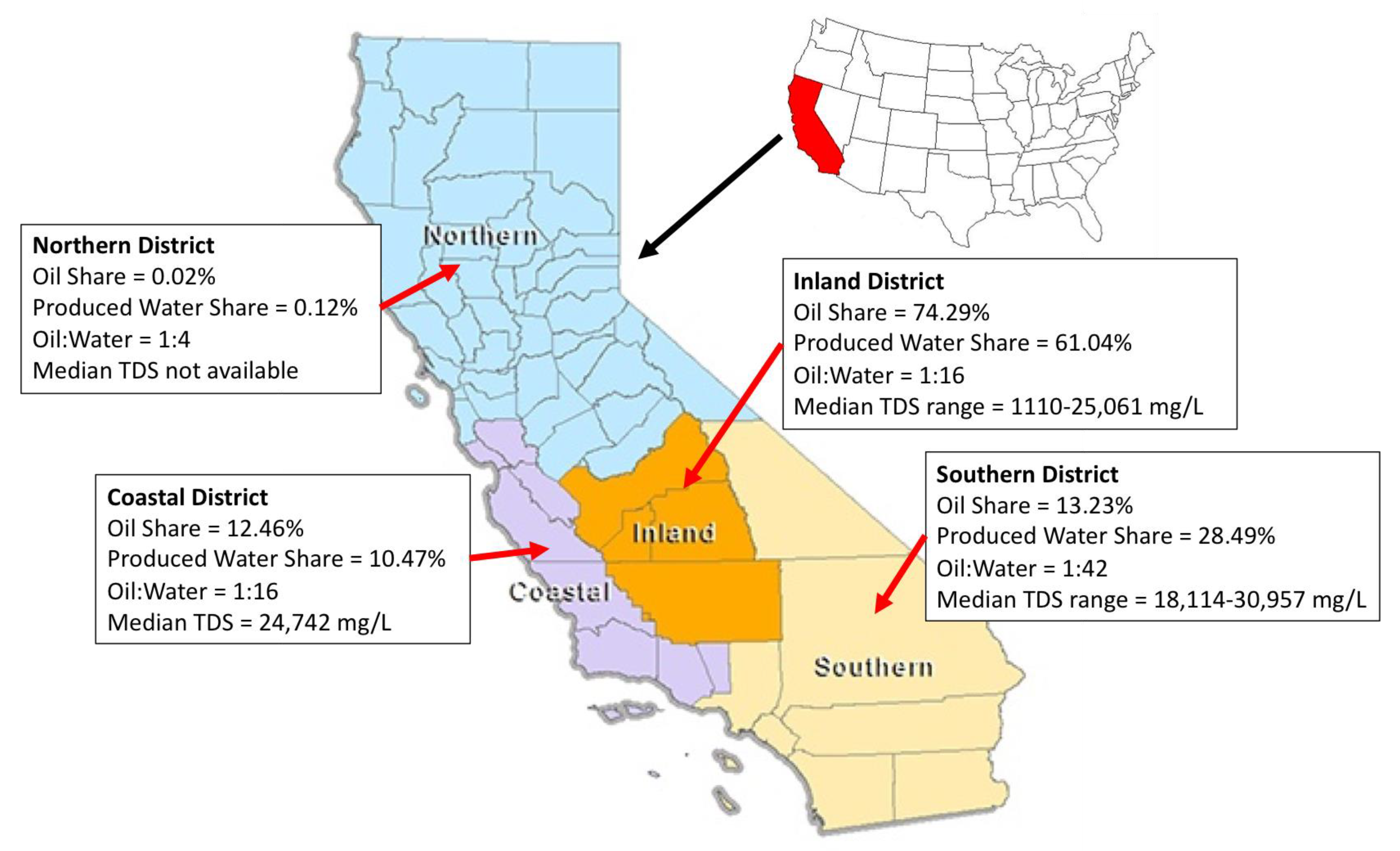
DOGGR (CalGEM) divides oil and gas operations across four districts: northern, inland, coastal, and southern. Figure 1 below graphically shows this division [3,4]. Over 74% of oil production in California takes place in the inland district (mainly in Kern County), while the balance comes in roughly equal proportions from the southern and coastal districts; very little oil is produced in the northern district (0.12%). Given the higher ratio of produced water to oil in the southern region compared to the coastal district, the share of produced water generation is approximately 61%, 29% and 10% for inland, southern, and coastal districts, respectively. On an annual basis, approximately 508.7 million cubic meters (3.2 million barrels) of produced water is generated across California.

The TDS concentration is used as the key water quality indicator by DOGGR (CalGEM) across various oil-producing regions in California and is also shown in Figure 1. While most produced waters in California have TDS concentrations above 15,000 mg/L, there are some regional variations, especially in the inland region. Typically, the fields east and southeast of the city of Bakersfield generate lower TDS produced waters (1000–16,000 mg/L) than the ones to the south and southwest (~13,000 to ~23,000 g/L) and those in the west and north west (~16,000 to ~25,000 g/L).

More detailed produced water quality data for these regions are provided in

Table 1. Detailed produced water qualities from select fields across different regions of California.

		Selected Samples Quality Overview
	Unit	Coastal		Southern	Inland
Parameter	mg/L	Santa Maria County	Ventura County		Low TDS	High TDS
TDS	mg/L	11,480	16,000	29,400	3500	23,000
Electrical Conductivity EC	mS/cm	16.4	23	42	5.4	37.3
pH	-	8.00	7.64	6.9	7.54	7.9
Chloride	mg/L	6500	9600	17,640	2100	13,800
Total Hardness	mgCaCO3/L	520	2599	1182	570	330
Calcium	mg/L	27	930	684	200	91
Magnesium	mg/L	5.8	41	504	18	25
Silica	mg/L	360	58	25	48	66
Oil and Grease *	mg/L	898	175	54	2.5	11
Total Petroleum Hydrocarbons (TPH)	mg/L	-	430	-	22	15
Sulfate	mg/L	130	30	2	1.5	840
Barium	mg/L	-	2.3	50.8	1.8	72.0
Strontium	mg/L	-	27	-	3.8	28
Iron	mg/L	1	2.3	1.54	1.9	ND
Total Suspended Solids (TSS)	mg/L	-	48	9.7	22	110
Turbidity	NTU	262	28	-	-	29
Total Organic Carbon (TOC)	mg/L	200	860	-	10	1
Hydrogen Sulfide (H2S)	mg/L	1.4	1.5	1.0	ND *	1.5
Boron	mg/L	-	52	25	3	72
Benzene, Toluene, Ethylbenzene, Xylene (BTEX	mg/L	-	-	-	5	1
Temperature	°F	104–158	80–100	140	80–100	Ambient
Gross Alpha Particles	pCi/L	-	41	-	-	-
Sodium Absorption Ration (SAR)	-	212	214	98	80–100	Ambient
Oil API	-	15.4	17	15	17	22

* ND: non-detect.

. These data were generated by the authors over the past few years from various produced water treatment projects and studies performed across California. While there are a wide range of concentrations for many parameters, the key indicators of “treatability” appear to be oil and grease, total petroleum hydrocarbons (TPH), hardness, silica, and boron in addition to TDS. The data shown for Santa Maria County and Ventura county in the Coastal district as well as the Southern district analysis are each a single sample. The data for the Inland district is shown as the lowest and highest TDS samples among a series of 15 samples. The variations are attributed to the diversity of the geochemical nature of the oilfields across the state. Standard measurement methods are provided in Appendix A.

3. California Water Reuse Standards

About 92% of the 508 million cubic meters (3.2 billion barrels) of produced water generated in California per year receives primary treatment (e.g., gravity separation to separate free oil from water) prior to re-injection, reuse or disposal. Approximately 20% of that volume (18.4% of the total volume) receives secondary treatment (typically, induced or dissolved gas flotation for emulsified oil and grease removal), and about 9% of that (1.8% of total) receives a tertiary level of treatment for beneficial reuse which may include different combinations of nutshell or other media filtration, ion-exchange softening and/or reverse osmosis desalination [2]. Currently, in California, there are no water quality standards developed for produced water reuse, primarily because it is happening less than 2% of the volume is beneficially reused, but also because there are a number of different beneficial reuse options. The three most common are: (1) direct onsite reuse for water or steam flooding, (2) agricultural irrigation, and (3) surface water (streamflow) augmentation. Hence, produced water reuse permits are considered on an ad hoc basis by the relevant local Regional Water Quality Control Board. If the water is returned to the same oil-bearing formation from which it came, there is no treatment required, but the injection well must be permitted.

Depending on the purpose of beneficial reuse purpose and permit requirements, the necessary treatment scheme is defined on a case-by-case basis. For example, reusing produced water in steam flooding operations requires different levels of softening, desilication and/or desalination to avoid premature scaling of the steam generating equipment. Once-through steam generators (OTSGs) can handle fairly high TDS concentrations (up to 10,000 mg/L) but require hardness and silica to be removed to very low levels to minimize scaling [2]. A key indicator of irrigation water quality is the sodium adsorption ratio (SAR); a high concentration of sodium relative to calcium and magnesium can lead to severe soil degradation issues (e.g., loss of permeability for clayey soils) [5]. The formulation for SAR is widely known and various crops have differing sensitivity to SAR as shown in

Table 2. Sensitivity of various crops to the SAR value.

Tolerance	SAR Range	Crop
Very Sensitive	2–8	Fruits, nuts, citrus, and avocado
Sensitive	8–18	Beans
Moderately tolerant	18–46	Clover, oats, rice
Tolerant	46–102	Wheat, barley, tomatoes, beets, tall wheat grass, crested grass

. Fruits, nuts, citrus and avocado crops are predominantly cultivated throughout California’s central valley and coastal regions [6,7].

Further, for reuse in agricultural irrigation, specific organic and/or inorganic constituents of concern may have to be removed to different levels depending on the type of the crop being irrigated. In particular, boron and chloride, which are present in various concentrations in produced waters across California, may need to be brought down to certain limits to protect crop yields. Boron, while an essential micronutrient for plant metabolism, has an extremely narrow concentration window where it changes from essential to toxic [8]. Excess boron (over 1 mg/L) and chloride (over 140 mg/L) concentrations in water can result in reduced yields of many food crops. Some examples of boron and chloride concentrations limits for various crops are provided in

Table 3. Chloride concentration impact on various classes of plants and crops.

Chloride Concentration (mg/L)	Impact	Susceptible Plant/Crop
Below 70	Safe for most plants	Rhododendron, azalea, blueberry, dry beans
70–140	Sensitive plants show injury	Onion, mint, carrot, lettuce, pepper, grape, raspberry
140–350	Moderately sensitive plants/crops	Potato, alfalfa, sudangrass, squash, wheat, sorghum, corn, tomato
Above 350	Can cause severe problems	Sugarbeet, barley, asparagus, cauliflower

and

Table 4. Boron concentration impact on various classes of plants and crops.

Boron Concentration (mg/L)	Impact	Susceptible Plants/Crops
Below 0.50	Extremely sensitive	Blackberry
0.50–0.75	Very sensitive	Peach, cherry, plum, grape, walnut, beans
0.75–1	Sensitive	Wheat, barley, lima bean, garlic, onion, lupine, strawberry, walnut
1–2	Moderately sensitive	Pepper, pea, carrot, radish, potato, cucumber
2–4	Moderately tolerant	Lettuce, cabbage, turnip, Kentucky bluegrass, oats, corn, mustard, clover, squash, muskmelon
4–6	Tolerant	Sorghum, tomato, alfalfa, vetch, sugarbeet, table beet
6–15	Very tolerant	Asparagus

[9].

4. Produced Water Treatment Process Design Considerations

Based on the data in Table 1, most California Central and Coastal basin produced waters have a TDS from ~3000 to 30,000 mg/L with a SAR between ~80 and >200, chloride between ~2000 and ~20,000 and boron from ~3 to ~70 ppm. Moreover, most California produced waters have significant amounts of both carbonate and non-carbonate hardness, including calcium, magnesium, barium and strontium; the non-carbonate hardness is predominantly associated with sulfate. In addition, most California produced waters contain high levels of silica and trace levels (single digit ppm values or lower) of iron and/or aluminum. Reviewing the produced water quality data and treatment objectives as outlined in the previous section, the primary contaminants of concern (CoCs) are SAR, boron and chloride; hence, most California produced water requires desalination for reuse in agricultural irrigation.

It is generally accepted that reverse osmosis (RO) is the most cost-effective, commercially proven technology for brackish water desalination [2,10,11]. The key element for reliable design and cost-effective operation of any RO process is the design and selection of an appropriate pre-treatment scheme to maximize recovery (reducing the amount of concentrated brine that is produced) and minimize the deleterious effects of RO membrane fouling, which include higher energy demand, down-time for cleaning, cleaning chemicals and premature membrane replacement. To avoid rapid fouling (loss of water permeability) of RO membranes, free and emulsified oil and grease (hexane extractable material or HEM, per US EPA1664B) and non-oil suspended solids (e.g., clay fines from the formation) need to be removed ahead of the RO process. Next, to avoid rapid degradation (loss of TDS rejection) of RO membranes, soluble hydrocarbons (e.g., alcohols, aldehydes, ketones) and volatile organic compounds (VOCs such as the sum of benzene, toluene, ethylbenzene, and xyelen or “BTEX”, diesel and gasoline range hydrocarbons) need to be removed ahead of the RO membrane process. Finally, to enable high recovery, sparingly soluble metals and minerals (e.g., iron and aluminum, silica, calcium carbonate, calcium, barium, and strontium sulfate) concentrations may need to be significantly reduced.

With appropriate pre-treatment, the RO membrane process operation is stable and consistent with little buildup in differential (feed-to-brine) or trans-membrane (feed-to-permeate) hydraulic pressure loss. After primary TDS reduction by RO, boron can still be well above the 1 mg/L maximum contaminant level required for agricultural irrigation. Boron chemistry in water is well established [12], but typically, at pH levels below ~9, boron predominantly exists as boric acid (B(OH)₃), which is poorly rejected by RO membranes because it is small, polar and uncharged. There are conflicting interpretations for the origin of the acidity of aqueous boric acid solutions. Raman spectroscopy of strongly alkaline solutions has shown the presence of B(OH)⁻₄ ions [13], leading some to conclude that the acidity is exclusively due to the abstraction of OH⁻ from water, according to [13,14,15]:

B(OH)₃ + 2H₂O ⇌ B(OH)⁻₄ + H₃O⁺  (K = 7.3 × 10⁻¹⁰; pK = 9.14)

(1)

And hence, above a pH of ~9, boric acid (B(OH)₃) forms borate (B(OH)₄⁻), which is rejected very highly (>90%) by most brackish water RO membranes [16]. As a result, depending on the concentration of boron in produced water, there may be a post-treatment polishing step may be required, comprising either: (a) boron selective ion-exchange resins or (b) a second pass of brackish water RO membranes with pH adjustment to about pH 10.

5. Pilot-Scale Case Study

The case study reported on herein is a two-month long field pilot test project performed in the DOGGR (CalGEM) Coastal District of California in 2018. The primary treatment objectives were to meet the beneficial reuse standards required by the neighboring agricultural end-users (see

Table 5. Key produced water quality and treatment objectives for this project.

Parameter	Unit	Raw Influent	Softened Influent	Treatment Objectives
TPH	mg/L	130	46	ND *
Oil and Grease	mg/L	95	1.5	ND
Turbidity	NTU	60	15	0.3
TDS	mg/L	~14,000	~15,000	1060
Hardness	mgCaCO3/L	~2400	~240	595
Alkalinity	mgCaCO3/L	~1000	~100	360
pH	-	7.3–7.5	8–9	6.90
Iron	mg/L	2.3	0.046	0.05
Manganese	mg/L	0.42	0.021	0.22
Calcium	mg/L	880	18	146
Magnesium	mg/L	41	23	56
Sodium	mg/L	~4500	4,500	86
Potassium	mg/L	480	480	5
Barium	mg/L	2.8	0.056	0.03
Chloride	mg/L	~7800	7800	72
Boron	mg/L	61	61	0.6
Sulfate	mg/L	37	37	367
Silica	mg/L	58	34.8	-
SAR	-	57	6	1.5

* ND: non-detect.

), while the secondary objective was to maximize the RO process recovery and minimize RO brine volumes because the cost of brine disposal in this region is exceptionally high (~$38 per m³; ~$6 per barrel). The pilot here had a throughput of 3.4 m³ per hour.

5.1. Produced Water Quality and Treatment Objectives

Table 5 outlines the concentrations of the key produced water quality parameters, as well as the treatment objectives for this project. The influent concentrations are single point measurements and the method and reporting limit (RL) for each parameter is shown in Appendix A. The treatment objectives were defined by the oil producer. From the information in Table 5, the principal COCs in the influent were:

• SAR
• Chloride
• Boron

Additionally, to protect RO membranes in operation, pre-treatment would need to be selected to target the removal of the following constituents:

• Oil and grease
• Suspended solids
• TPH and other dissolved organic constituents
• Hardness and alkalinity
• Sparingly soluble metals and minerals

5.2. RO Pretreatment Process Design

The raw influent and softened influent water quality from Table 5 was modeled to evaluate scale formation potential using Genesys International’s MM4 software. A number of minerals were supersaturated such that catastrophic scaling would be expected at only 10% product water recovery (

Table 6. Supersaturated mineral salts and their saturation levels in the influent. RO: reverse osmosis.

Mineral Salt	% Saturation in Raw Water @ 10% Recovery	% Saturation in Softened Feed Water	% Saturation in RO Brine @ pH 6.5 and 70% Recovery	% Saturation in RO Brine @ 70% Recovery with Anti-Scalant
CaCO3	163%	33%	76%	39%
BaSO4	381%	16%	57%	1%
Fe(OH)3	2221%	25%	98%	7%
Mn(OH)2	135%	3%	13%	1%
SiO2	54%	29%	99%	66%

). This includes mineral species of CaCO₃, BaSO₄, Fe(OH)₃, Mn(OH)₂ and SiO₂. Since there was both carbonate and non-carbonate hardness, lime-soda softening was evaluated. The lime-soda softened water was well below saturation for all the relevant minerals, and when adjusted to pH 6.5 none of the minerals exceeded their saturation concentrations up to 70% recovery. With proper anti-scalant addition, all metals and minerals remain well below saturation levels up to 70% recovery and with slightly higher Anti-Scalant dosing up to 84% recovery (not shown).

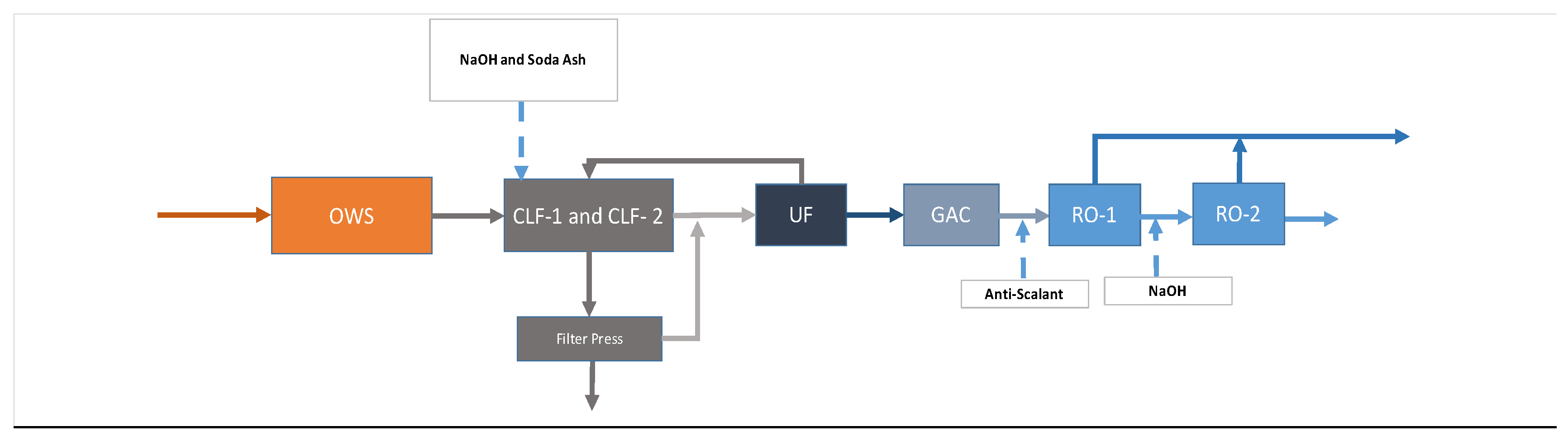
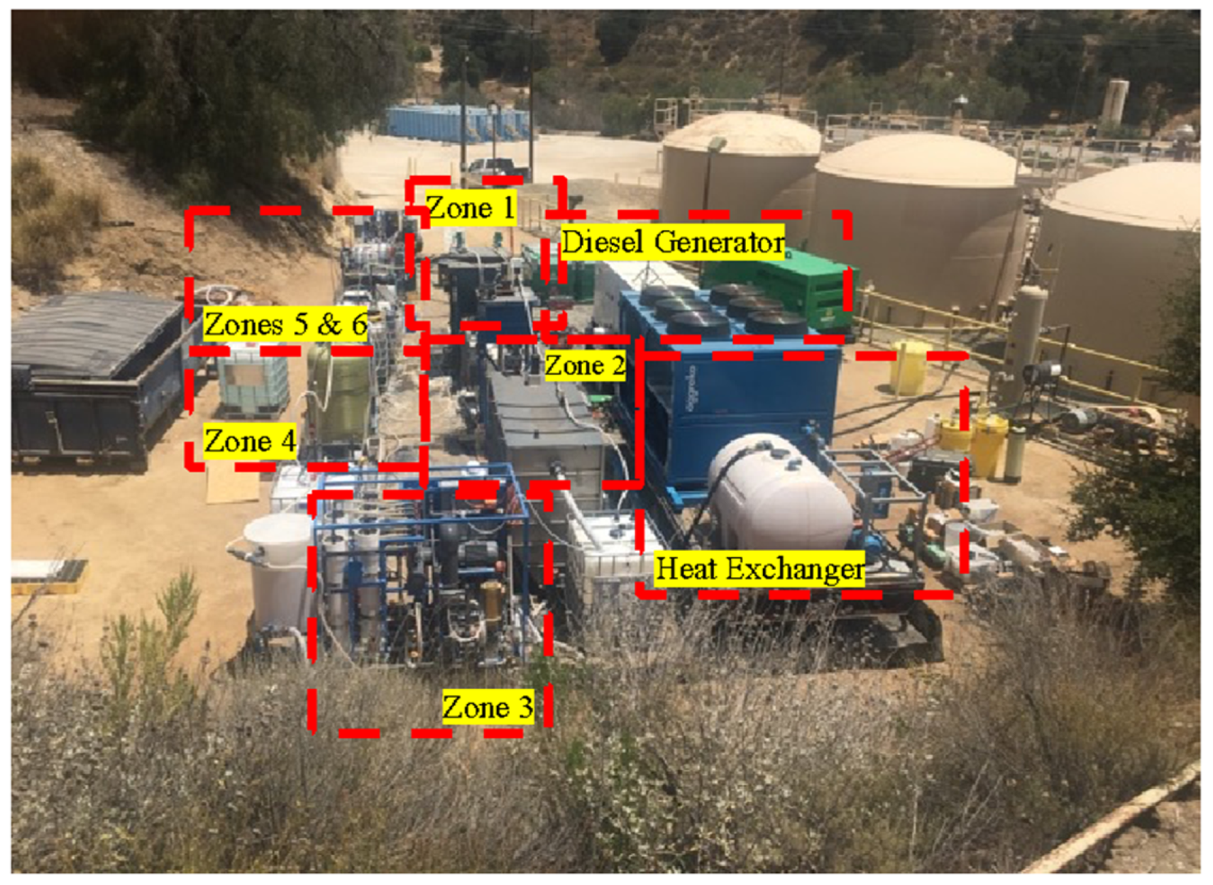
Accordingly, after a review of multiple technologies [2], it was decided that upfront chemical softening followed by TSS removal would sufficiently lower the scaling and fouling potential of the produced water such that it could be treated by RO at sufficiently high recovery [75–80%]. The process included an upfront oil–water separator to manage inevitable variations in oil and grease and soluble hydrocarbons, in addition to improving the efficiency of the chemical softening process. An intermediate ultrafiltration (UF) membrane filtration system was used downstream of chemical softening, which significantly lowered the particulate fouling potential of the RO feed, providing an absolute barrier to TSS above 10 nm. Additionally, granular activated carbon (GAC) was employed to remove soluble hydrocarbons that could rapidly damage RO membranes. Using the above process design approach, the treatment process proposed and deployed for the pilot was divided into six operating zones detailed below. A process flow diagram is shown in Figure 2. A picture of the pilot site (approximately 9000 ft² in area) is shown in Figure 3.

• Zone 1: Oil–Water Separation (OWS)

  ∘

  Concept and intended function: Absorb variations in and remove free oil and grease to improve the operation of downstream unit operations

  ∘

  Key components: A feed pump and a coalesce-based oil water separation unit

  ∘

  Treatment objective: 90% free oil and grease removal

  ∘

  Key unit operation: Custom made

• Zone 2: Chemical Softening/Sedimentation System

  ∘

  Concept and intended function: Remove hardness using a two-stage approach; initially increasing the pH (using sodium hydroxide) to remove carbonate hardness followed by adding soda ash to remove non-carbonate/metallic hardness

  ∘

  Key components: A feed pump, followed by two flocculation/clarification units (CLF-1 and CLF-2) each having a dosing station, a flocculation chamber and a clarification chamber

  ∘

  Treatment objective:

  ▪

  Overall hardness removal: 95%

  ▪

  Iron removal: 50%

  ▪

  Silica removal: 30%

  ▪

  Remaining oil and TSS: 50%

  ∘

  Key unit operation:

  ▪

  CLF-1: MW Watermark, model: SPC-20,

  ▪

  CLF-2: Custom-made by Muerer Research, Inc.

• Zone 3: Suspended Solids Polishing

  ∘

  Concept and intended function: To remove the suspended and aggregated solids, thereby pretreating the water. The intended filtrate quality would have low turbidity and negligible suspended solids.

  ∘

  Key components: A polymeric ultrafiltration (UF) membrane system with standard spiral wound membrane module form factor. The system operated in a feed-and-bleed mode, with a fixed concentration factor and recirculation ratio. The membranes were back-washable

  ∘

  Treatment objective: 98% TSS and oil removal, 20% hardness removal

  ∘

  Key unit operation: Water Planet Inc., model: PC-6.

• Zone 4: Dissolved Hydrocarbon Removal

  ∘

  Concept and intended function: An additional pretreatment step to remove dissolved hydrocarbons and other organics from the influent to protect the downstream unit operations from fouling

  ∘

  Keu components: A break/feed tank, a feed pump, followed by a granular activated carbon (GAC) filter

  ∘

  Treatment objective: 99% dissolved organics and TPH removal

  ∘

  Key unit operation: Water Planet Inc., model: PC-6.

• Zone 5: Reverse Osmosis (RO) Desalination

  ∘

  Concept and intended function: To remove the remaining dissolved solids in the water, attaining a permeate quality and recovery, meeting treatment objectives and economic benchmarks

  ∘

  Key components: two RO units in series:

  ▪

  First stage (RO-1) intended for general TDS removal consisting of a break tank, a dosing stations for anti-scalant chemistry, and a high-pressure brackish water RO unit

  ▪

  Given the high boron concertation of the influent, a second stage RO (RO-2) was added to further reduce boron to below 0.6 mg/L. The platform also consisted of a break tank and a dosing station to add sodium hydroxide for pH adjustment to the 10.0–10.5 range to maximize boron rejection.

  ∘

  Treatment objective:

  ▪

  RO-1: 98% TDS removal, 80% boron removal

  ▪

  RO-2: 40% TDS removal, 95% boron removal

  ∘

  Key unit operation:

  ▪

  RO-1: GE, model: E-Series Ultra E4

  ▪

  RO-2: Applied Membranes, Inc., model: J-12

• Zone 6: Solid Waste Management

  ∘

  Concept and intended function: To dewater the solid slurries from clarifiers and dramatically reduce the solid waste generation volumes

  ∘

  Key components: A slurry/feed tank, a transfer pump, and a filter press (FP)

  ∘

  Treatment objective: Produce a solid cake with only up to 40–50% wetness

  ∘

  Key unit operation: MW Watermark, Model: FP470G32L-7/14-1/2MXX

5.3. Field Performance Results

5.3.1. Influent and Treated Water Quality

Throughout the pilot, the water quality parameters listed in

Table A1. List of onsite analysis, methods and reporting limits.

Parameter	Instrument/Method	Reporting Limit	Unit
Electrical Conductivity (EC)	Hach instrument, model HQ40D	2	μS/cm
pH	Hach instrument, model HQ40D	0.10	-
Total Hardness	Hach instrument, model 5-EP test kit	17.5	mgCaCO3/L
Oil and Grease	Hexane extraction method using a Turner Design instrument TD-500	5	mg/L
Turbidity	Hach 2100Q	0.25	NTU
Silica	Hach silica HR reagent pack using a Hach DR1900 spectrophotometer	1	mg/L
Boron	Hach boron TNTplus vial test using a Hach DR1900 spectrophotometer	0.05	mg/L
Iron	Hach FeeroVer® reagent using a Hach DR1900 spectrophotometer	0	mg/L

in Appendix A at the inlet and outlet of each zone were monitored at a regular interval using field instruments onsite. Further, a more detailed offsite analysis of minerals and organic constituents of the influent produced water and treated product water were performed on a weekly basis. See Appendix A (

Table A2. List of offsite analysis, methods and reporting limits.

Parameter	Method	Reporting Limit	Unit
Ammonia, unionized as N	-	1.7	mg/L
Ammonium as N	Calculation	0.10	mg/L
Oil and Grease by EPA1664	EPA1664	5.0	mg/L
Fluoride by EPA300.0	EPA300.0	2.0	mg/L
Nitrate as NO3 EPA300.0	EPA300.0	9.0	mg/L
Nitrite as NO2 by EPA 00.0	EPA300.0	6.6	mg/L
Phosphate, ortho as P by EPA300.0	EPA300.0	2.0	mg/L
Sulfate by EPA300.0	EPA300.0	2.0	mg/L
TPH	EPA8015M	2.6	mg/L
Sulfide, dissolved by EPA9034M	EPA9034M	2.00	mg/L
9040B pH	EPA9040B/SM4500H + B	0.10	-
Color	SM2120B	3.0	Color unit
Turbidity	SM2130B	0.25	NTU
Alkalinity	SM2320B	10	mgCaCO3/L
Total Petroleum Hydrocarbon (TPH)	EPA8015M	0.1	mg/L
Total Oil and Grease	EPA1664	5	mg/L
Turbidity	SM2130 B	0.25	NTU
Total Dissolved Solids (TDS)	SM2540C	10	mg/L
Electrical Conductivity (EC)	SM2510B	2	μS/cm
Total Hardness	EPA200.7	0.21	mgCaCO3/L
Alkalinity	SM2320B	10	mgCaCO3/L
pH	EPA9040B/SM4500	10	-
Iron	EPA200.7	0.050	mg/L
Manganese	EPA200.7	0.01	mg/L
Calcium	EPA200.7	0.10	mg/L
Magnesium	EPA200.7	0.050	mg/L
Sodium	EPA200.7	25	mg/L
Potassium	EPA200.7	0.50	mg/L
Barium	EPA200.7	0.010	mg/L
Strontium	EPA200.7	0.010	mg/L
Total Suspended Solids (TSS)	SM2540D	10	mg/L
Total Organic Carbon (TOC)	SM5310B	0.5	mg/L
Hydrogen Sulfide (H2S)	HACH HS-C	0.1	mg/L
Temperature	EPA170.1/SM2550B	1.0	°C
Gross Alpha Particles	SM7110C-11	1.66	pCi/L
Oil API	ASTM D287/D1298	0.10	-
Chemical Oxygen Demand	SM5220D	0.2	mg/L
Phenols, Total	SM5530 and EPA420.1	0.25	mg/L
Chloride by EPA 300.0	EPA300.0	0.4	mg/L
Bromodichloromethane	EPA8260B/LUFT	0.1	mg/L
Xylenes (total)	EPA8260B/LUFT	0.1	mg/L
Bromoform	EPA8260B/LUFT	0.1	mg/L
Bromomethane	EPA8260B/LUFT	0.1	mg/L
n-Butylbenzene	EPA8260B/LUFT	0.1	mg/L
sec-Butylbenzene	EPA8260B/LUFT	0.1	mg/L
tert-Butylbenzene	EPA8260B/LUFT	0.1	mg/L
Carbon tetrachloride	EPA8260B/LUFT	0.1	mg/L
Chlorobenzene	EPA8260B/LUFT	0.1	mg/L
Chloroethane	EPA8260B/LUFT	0.1	mg/L
Chloroform	EPA8260B/LUFT	0.1	mg/L
Chloromethane	EPA8260B/LUFT	0.1	mg/L
2-Chlorotoluene	EPA8260B/LUFT	0.1	mg/L
4-Chlorotoluene	EPA8260B/LUFT	0.1	mg/L
Dibromochloromethane	EPA8260B/LUFT	0.1	mg/L
1,2-Dibromo-3-chloropropane	EPA8260B/LUFT	0.1	mg/L
1,2-Dibromoethane (EDB)	EPA8260B/LUFT	0.1	mg/L
Dibromomethane	EPA8260B/LUFT	0.1	mg/L
1,2-Dichlorobenzene	EPA8260B/LUFT	0.1	mg/L
1,3-Dichlorobenzene	EPA8260B/LUFT	0.1	mg/L
1,4-Dichlorobenzene	EPA8260B/LUFT	0.1	mg/L
Dichlorodifluoromethane	EPA8260B/LUFT	0.1	mg/L
1,1-Dichloroethane	EPA8260B/LUFT	0.1	mg/L
1,2-Dichloroethane	EPA8260B/LUFT	0.1	mg/L
1,1-Dichloroethene	EPA8260B/LUFT	0.1	mg/L
cis-1,2-Dichloroethene	EPA8260B/LUFT	0.1	mg/L
trans-1,2-Dichloroethene	EPA8260B/LUFT	0.1	mg/L
1,2-Dichloropropane	EPA8260B/LUFT	0.1	mg/L
1,3-Dichloropropane	EPA8260B/LUFT	0.1	mg/L
2,2-Dichloropropane	EPA8260B/LUFT	0.1	mg/L
1,1-Dichloropropene	EPA8260B/LUFT	0.1	mg/L
cis-1,3-Dichloropropene	EPA8260B/LUFT	0.1	mg/L
trans-1,3-Dichloropropene	EPA8260B/LUFT	0.1	mg/L
Ethylbenzene	EPA8260B/LUFT	0.1	mg/L
Hexachlorobutadiene	EPA8260B/LUFT	0.1	mg/L
4-Isopropyl Toluene	EPA8260B/LUFT	0.1	mg/L
Isopropylbenzene	EPA8260B/LUFT	0.1	mg/L
Benzene	EPA8260B/LUFT	0.1	mg/L
Methylene chloride	EPA8260B/LUFT	0.1	mg/L
Naphthalene	EPA8260B/LUFT	0.1	mg/L
n-Propylbenzene	EPA8260B/LUFT	0.1	mg/L
Bromobenzene	EPA8260B/LUFT	0.1	mg/L
Styrene	EPA8260B/LUFT	0.1	mg/L
1,1,1,2-Tetrachloroethane	EPA8260B/LUFT	0.1	mg/L
1,1,2,2-Tetrachloroethane	EPA8260B/LUFT	0.1	mg/L
Tetrachloroethene (PCE)	EPA8260B/LUFT	0.1	mg/L
Toluene	EPA8260B/LUFT	0.1	mg/L
1,2,3-Trichlorobenzene	EPA8260B/LUFT	0.1	mg/L
1,2,4-Trichlorobenzene	EPA8260B/LUFT	0.1	mg/L
1,1,1-Trichloroethane	EPA8260B/LUFT	0.1	mg/L
1,1,2-Trichloroethane	EPA8260B/LUFT	0.1	mg/L
Dibromofluoromethane	EPA8260B/LUFT	0.1	mg/L
4-Bromofluorobenzene	EPA8260B/LUFT	0.1	mg/L
Toluene-d8	EPA8260B/LUFT	0.1	mg/L
Bromochloromethane	EPA8260B/LUFT	0.1	mg/L
Trichloroethene (TCE)	EPA8260B/LUFT	0.1	mg/L
Trichlorofluoromethane	EPA8260B/LUFT	0.1	mg/L
1,2,3-Trichloropropane	EPA8260B/LUFT	0.1	mg/L
1,2,4-Trimethylbenzene	EPA8260B/LUFT	0.1	mg/L
1,3,5-Trimethylbenzene	EPA8260B/LUFT	0.1	mg/L
Vinyl chloride	EPA8260B/LUFT	0.1	mg/L
Naphthalene	EPA8270-SIM	10	mg/L
Phenanthrene	EPA8270-SIM	10	mg/L
Bromide	EPA300.0	20	mg/L

) for a complete list of onsite and offsite analysis and methods used and Appendix B for a list of the number of samples by location and water quality parameter. While most influent concentrations remained fairly stable during the course of the pilot, the influent oil and grease concentrations varied significantly with daily onsite measurements varying from as low as 8 mg/L to as high as 1013 mg/L. The variations in the oil grease content can be attributed to the efficacy of primary separators and/or feed level changes during the day. Typically, the lower the feed tank, the more oil from the skimmed oil layer on the top gets into the influent. This is why any advanced produced water treatment system requires a robust oil/water separator as the first step in the treatment process to be able to absorb these variations and protect the downstream unit operations and their efficiency. The treated water parameters, however, were stable and far exceeded the treatment objectives.

5.3.2. Separation Performances by Each Zone

Table 7. Changes in concentrations of water quality parameters across different process unit operations.

Parameter	Unit	OWS Feed	CLF-1 Feed	CLF-2 Feed	UF Feed	GAC Feed	RO-1 Feed	RO-2 Feed	Product	Treatment Objective
Electrical Conductivity	mS/cm	22.26	22.39	22	22	23	22	0.40	0.23
pH	-	7.63	10.50	9.04	9.60	9.62	9.54	10.71	10.94	6.9
Oil and Grease	mg/L	106	36	0.00	1.57	0.21	0.00	0.00	0.00	ND
Turbidity	NTU	52.57	70.13	34.70	14	0.60	0.63	0.50	0.31	0.3
Hardness	mgCaCO3/L	2437		1716	492	327		ND	ND	595
Calcium	mg/L	1125			11				ND	146
Magnesium	mg/L	42			21.75				ND	56
Barium	mg/L	2.4			0.08				ND	0.03
Strontium (mg/L)	mg/L	33.25			1.99				ND	-
Iron (mg/L)	mg/L	0.87		0.24	0.08	0.03	0.00	0.00	0.00	0.05
Silica (mg/L)	mg/L	35.88		26.80	19.62		19.21	0.00	0.00	-
Boron (mg/L)	mg/L	56.74					54.80	5.45	0.29	0.6
TPH (mg/L)	mg/L					46	0.20		ND	ND
BTEX (mg/L)	mg/L					2.70	0.00		ND	-
TDS	mg/L								135	1060

outlines the changes in concentrations of different water quality parameters across different process zones versus the treatment objective for each parameter. The number of samples taken at each event, as well as the standard error calculated using Microsoft Excel divided by the total number samples for each case, have been reported in Appendix B. The concentrations shown are the averages of analyses done over the course of the pilot. Taking these values into account, the removal efficiencies of various categories of contaminants by each zone have been calculated and are shown in

Table 8. Summary of unit operations performances and key process indicators.

Unit Operation	Performance Metric	Average Pilot Results	Notes
OWS	Oil Removal	71%
	TSS Removal	-
CLF	Hardness Removal	87%	Average Sodium Hydroxide Dose = 1078 mg/L
	Iron Removal	98%	Average Soda Ash Dose = 1200 mg/L
	Silica Removal	43%	Solid Generation Rate = 0.35 lbs/barrel (0.99 kg/m3) of feed
	Oil Removal	97%
	Gross Alpha Particles	91%
	TSS removal	84%
UF	TSS Removal	95%	Average Feed Pressure = 10.4 psi (0.70 bar)
	Oil Removal	100%	Average Flux = 25 LMH
	Hardness	22%	Specific Energy Consumption (SEC) = 0.041 kWh/barrel of feed (0.258 kwh/m3 of feed)
			One Clean-in-Place per week
GAC	Dissolved Organic Compound (DOC)/TPH removal	100%	5 ft3 media per gpm, not breakthrough observed
RO-1	Recovery	65%	Average Feed Pressure = 688 psi (46.80 bars)
	Hardness Removal	100%	Average Recovery = 68% *
	TDS Removal	99%	Anti-Scalant dose = 8 mg/L
	Boron Rejection	88%	SEC = 0.24 kWh/barrel of feed (1.50 kWh/m3 of feed)
RO-2	Recovery	90%	Average Feed Pressure = 135 psi (9.18 bar)
	TDS Removal	30%	Average Recovery = 91%
	Boron Rejection	94%	Average Sodium Hydroxide Dose = 193 mg/L

* RO feed pump limitation.

. Key process parameters for each zone are also presented in Table 8. These are the key parameters needed to size the solution at larger scales.

5.4. Capital and Operating Costs

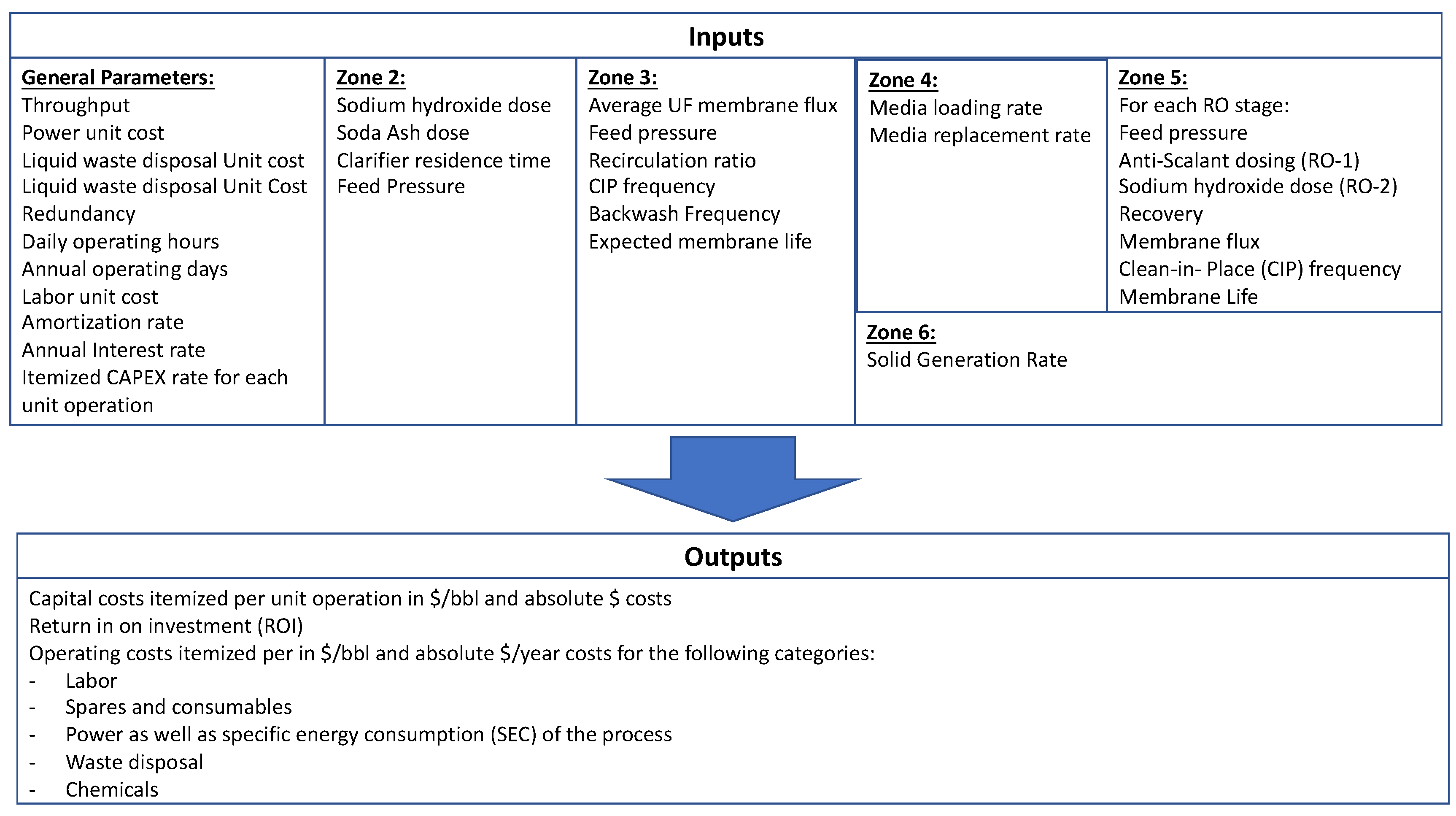
A cost model was developed that uses the data from the pilot results to estimate capital and operating costs (CAPEX and OPEX, respectively) at larger scales. Figure 4 shows the working diagram of the model. Using this model for the conditions defined in

Table 9. General scale up assumption.

Parameter	Value	Unit
Blowdown Flow Rate	2436	m3/day
	15,326	barrels per day
Annual Operating Days	365	days
Daily Operating Hours	24	hours
Cost of Electricity	$0.11	$/kWh
Liquid Waste Disposal Cost	$0.75	$/m3
Solid Waste Disposal Cost	$0.38	$/m3
Amortization Period	5	years
Annual Interest Rate	6%	%

, we estimated CAPEX and OPEX for the following scenarios:

• Scenario 1: Baseline similar to the pilot process configuration
• Scenario 2: Baseline with a 5% UF filtrate blend to take advantage of the good quality of the permeate and reduce some of the capital and operating costs
• Scenario 3: Blend with membrane-based RO concentrate treatment

The throughput considered in Table 9 is typical for most small to mid-sized producers across California. The resulting CAPEX and OPEX are shown in

Table 10. Scale up normalized CAPEX and operating cost (OPEX) for each scenario.

Configuration	Recovery (%)	CAPEX	OPEX	Total
		$/m3 Influent	$/m3 Influent
Scenario 1	80	$0.75	$0.76	$1.50
Scenario 2	82	$0.74	$0.69	$1.43
Scenario 3	95	$0.91	$0.70	$1.60

.

Generally, increasing the overall process recovery seems to reduce the overall operating costs through savings in waste management costs. Solely from a pure cost perspective (CAPEX plus OPEX), Scenario 2 seems to be the most cost effective of the three evaluated. That said, there are several life cycle and intangible costs associated with having to manage less brine volume which are not included in this estimate. For example, less brine volume to dispose of means more disposal well capacity and lifetime. It also means smaller downstream infrastructure such as tanks, pumps, and pipeline and more available fresh water. The OPEX breakdown per category is provided in

Table 11. OPEX breakdown in $/m³ of influent per scenario.

OPEX Item	Scenario 1	Scenario 2	Scenario 3
Chemicals	$0.15	$0.16	$0.28
Power	$0.05	$0.05	$0.11
Waste Mgmt.	$0.44	$0.38	$0.19
Spares	$0.09	$0.08	$0.10
Labor	$0.02	$0.02	$0.02
Total	$0.76	$0.69	$0.70

.

6. Conclusions

From the 508.7 million cubic meters (3.2 billion barrels) of produced water generated annually in California, only 8% receives some form of advanced treatment for beneficial reuse. Tightening regulations, California’s limited access to freshwater resources (especially in oil-producing regions), and the proximity of most oilfields to farmlands will likely increase the demand for beneficial reuse. The majority of produced water qualities across California have high TDS levels. Comparing that and other inorganic and organic parameters against some of the requirements for agricultural water and regulations, advanced treatment in the form of membrane-based desalination (specifically RO) seems to be the most cost-effective and commercially available solution. For membrane-based desalination to operate sustainably here, care must be given to the design of the pre-treatment. The main categories of contaminants that need to be addressed are free oil and greases, suspended solids, dissolved organics and hydrocarbons, hardness and inorganic salts, and silica. Boron is another parameter that is universally present at potentially toxic levels in produced waters across California. In order to being boron down to acceptable levels, consideration needs to be given to boron chemistry and membrane rejection when designing the RO component of the process. Finally, using data from an actual pilot project, our economic model show that the combined capital and operating cost of advanced treatment of high hardness, high TDS brackish produced water is within $1.43 to $1.46 per each m³ of produced water treated. This may be higher than the current cost of fresh water (typically in the range of $0.49–0.92 per m³), but certainly an affordable option when considering all the regulatory, limited disposal infrastructure, and rising costs of water management such as transportation to other disposal sites.

References

- California Geologic Energy Management Division online Data. Available online: https://www.conservation.ca.gov/calgem (accessed on 19 May 2020).
- Wang, J.; Hancock, A.D.; Wang, J.; Bhattacharjee, S.; Edalat, A. Produced Water Management in Upstream Oil and Gas Production; Hoek, E.M.V., Ed.; Morgan Claypool Publishers: LaPorte, CO, USA, 2020. [Google Scholar]
- Metzger, L.F.; Landon, M.K. Preliminary Groundwater Salinity Mapping Near Selected Oil Fields using Historical Water-Sample Data; U.S. Geological Survey Numbered Series; U.S. Geological Survey: Sacramento, CA, USA, 2018. Available online: https://pubs.usgs.gov/sir/2018/5082/sir20185082_.pdf (accessed on 23 June 2020).
- CalGEM-Districts-Map. Available online: ftp://ftp.consrv.ca.gov/pub/oil/GIS/MapsPDF/CalGEM-Districts-Map.pdf (accessed on 1 June 2020).
- Aboukarima, A.M.; Al-Sulaiman, M.A.; Marazky, M.S.A.E. Effect of sodium adsorption ratio and electric conductivity of the applied water on infiltration in a sandy-loam soil. Water SA 2018, 44, 105–110. [Google Scholar] [CrossRef]
- SAR Hazard of Irrigation. Available online: https://www.lenntech.com/applications/irrigation/sar/sar-hazard-of-irrigation-water.htm (accessed on 19 May 2020).
- ANZECC & ARMCANZ (2000) Water Quality Guidelines. Available online: https://www.waterquality.gov.au/anz-guidelines/resources/previous-guidelines/anzecc-armcanz-2000 (accessed on 2 June 2020).
- Brdar-Jokanovic, M.A. Boron Toxicity and Deficiency in Agricultural Plants. Int. J. Mol. Sci. 2020, 21, 1424. [Google Scholar] [CrossRef] [PubMed]
- Hopkins, B.G.; Horneck, D.A.; Stevens, R.G.; Ellsworth, J.W.; Sullivan, D.M. Managing Irrigation Water Quality; A Pacific Northwest; Extension Publication, August 2007. Available online: https://catalog.extension.oregonstate.edu/sites/catalog/files/project/pdf/pnw597.pdf (accessed on 23 June 2020).
- Bhojwani, S.; Topolski, K.; Mukherjee, R.; Sengupta, D.; El-Halwagi, M.M. Technology review and data analysis for cost assessment of water. Sci. Total Environ. 2019, 651, 2749–2761. [Google Scholar] [CrossRef] [PubMed]
- Youssef, P.G.; Al-Dadah, R.K.; Mahmoud, S.M. Comparative Analysis of Desalination Technologies. Energy Prodecia 2014, 61, 2604–2607. [Google Scholar] [CrossRef]
- Kochkodan, V.; Bin Darwish, N.; Hilal, N. The Chemistry of Boron in Water; Elsevier: Amsterdam, The Netherland, 2015; ISBN 978-0-444-63454-2. Available online: https://www.researchgate.net/publication/295858025_THE_CHEMISTRY_OF_BORON_IN_WATER (accessed on 23 June 2020).
- Jolly, W.L. Modern Inorganic Chemistry; McGraw-Hill: New York, NY, USA, 1984; p. 198. ISBN 978-0070327603. [Google Scholar]
- Housecroft, C.E.; Sharpe, A.G. Inorganic Chemistry, 2nd ed.; Pearson Prentice-Hall: New Jersey, NJ, USA, 2005; p. 135. ISBN 978-013039913. [Google Scholar]
- Hayne, M.H. Comprehensive Chemistry for JEE advanced 2014; Tata McGraw Hill Education: New York, NY, USA, 2014; p. 15. ISBN 978-1-259-06426-5. [Google Scholar]
- Wilf, M.; Park, J.S.; Brown, J. Boron Rejection by Reverse Osmosis Membranes: National Reconnaissance and Mechanism Study; U.S. Bureau of Reclamation Report No. 127; 2009. Available online: https://www.usbr.gov/research/dwpr/reportpdfs/report127.pdf (accessed on 23 June 2020).
© 2020 by the authors. Licensee MDPI, Basel, Switzerland. This article is an open access article distributed under the terms and conditions of the Creative Commons Attribution (CC BY) license (http://creativecommons.org/licenses/by/4.0/).