Perspectives of Water Distribution Networks with the GreenValve System

Abstract

In recent years, water utilities have made worldwide investments targeted to the implementation of an effective monitoring system and the installation of pressure-reducing valves in strategic nodes of water distribution networks. In fact, these interventions are considered fast and effective solutions to address at least two main concerns of modern water utilities: leakage reduction and energy efficiency. The present paper, on the basis of a database of working conditions of installed pressure-reducing valves, discusses the range of applicability of the GreenValve system (GVS) as an alternative solution to improving standard pressure-reducing valve capabilities. The device is able to recover energy, and it can be used to create a stand-alone monitoring node with remote control ability, optimizing the network from an energetic, functional, and hydraulic point of view.

1. Introduction

Water distribution network (WDN) optimization has attracted the attention of researchers in the last few decades. The reduction of water leakages and the reduction of energy consumption are two of the water industry’s main concerns. Water leakage in a pipeline, besides being an environmental problem, is an economic and energy efficiency issue. One of the most common solutions to reduce leakages is the installation of pressure-reducing valves (PRVs) to apply pressure management strategies [1]. This solution is often favored by managers because it gives effective results and avoids structural interventions such as pipeline revamping, which is often difficult to realize in urban areas. A clear review of the methods for leakage control can be found in [2], where pressure management is identified as the only method that can effectively reduce background leakage. Some researchers have been looking for procedures to find the best placement of PRVs in a network [3,4,5,6,7,8,9,10] to obtain maximum effectiveness from the operation; others have incorporated leakage terms and effects of valve control in the same network model [11,12,13,14] to find the best solution.

One of the prerequisites for these kinds of procedures is the availability of an efficient and widespread monitoring system to gather information about the real functioning of the WDN [15]. Subdividing the network into smaller monitored areas, commonly called district monitoring areas (DMAs) [16,17], is a widely-used method to manage pressure and improve control. DMAs have proved to be a viable solution for the reduction of water leakages and demand [18].

To create a DMA, it is necessary to install control valves to isolate the district as well as sensors to monitor the flow rate [19]. The case discussed in [20] demonstrates that dynamic management of the DMA patterns based on water demand (e.g., for day and night periods) can improve the energetic efficiency of the WDN and drastically reduce leaks. Nevertheless, dynamic DMA management requires a wide monitoring of the system, created with a network of pressure transducers and flow meters, and the use of smart devices able to react to real-time managing strategies.

Some innovative pressure management strategies have been experimented on in [20,21,22,23,24]. The latter considered the possibilities of a real-time pressure control of the network based on measurements in critical nodes. The authors [20,21,22,23,24] underlined that the two main prerequisites to use such innovative strategies are sufficient historical series of pressure and flow rate at some points of the net and the use of smart control valves. Smart control valves are devices that can be controlled remotely and have the possibility of being programmed.

Many of the pressure management strategies that can be applied to WDNs require the use of PRVs. Consequently, their number is constantly increasing, and with them, the amount of energy dissipated for the management of the network. An analysis of the amount of energy dissipated by PRVs is provided in Section 2.

In cases where PRVs dissipate a large amount of energy, turbine systems can be a suitable solution to recover energy. There are various examples of devices that can be used to this end. Cross-flow turbines (also called Banki turbines) are typically used in water supply systems in atmospheric discharge points [25]. This type of turbine is particularly convenient because of its simplicity of design and construction and high-efficiency guarantees for a large range of operating conditions [26]. Another kind of machinery that can be used in pressurized pipelines is pump as turbine (PAT) [27]. This device consists of a pump installed in a reverse mode that recovers energy instead of consuming it. In [28], PATs are defined as an efficient and inexpensive tool to recover power with small pressure heads for flow rates with a variable trend. Even though these hydraulic machines allow energy recovery, they cannot control the discharges efficiently (except in a few cases and in small quantities), requiring additional infrastructure [29], such as a bypass with a PRV working in parallel.

Most modern pressure management strategies require the introduction of new and improved devices to regulate the pressure in the network. Moreover, monitoring devices that allow real-time monitoring, like flow meters and pressure transducers, are also needed. In the present paper, we discuss the possibility of using an innovative device able to control the flow and recover part of the energy necessary to dissipate. The device concept and first release have been previously presented in [30]. The GreenValve system (GVS) is a device able to substitute a PRV to provide many additional functionalities useful for the optimization of network management. In particular, GVS uses recovered energy to enable the remote control of the valve and the remote real-time monitoring of pressure and flow rates without the necessity of further devices and electric connection. Additionally, a surplus of recovered energy can be used for the electric supply of other local devices, for example, a booster pump for the injection of disinfectant, water quality sensors, or simply for the lighting of the inspection chambers where the valve is installed.

Study Methodology

The main purpose of the study is the evaluation of the applicability of GVS in WDNs.

The first part of the paper discusses the energy that is usually dissipated in common pressure-reducing valves, considering a dataset of PRV working conditions, collected from real installations or models and reported in Appendix A.

Based on the first classification of the PRVs, focused on the energy dissipated by each valve, the possible installation of energy recovery devices is examined through a preliminary economic analysis. The analysis evaluates the PRVs that can be substituted for energy production and the PRVs that are not appropriate for this scope but can, instead, show the application range of the GVS. Then, the possible applications of the GVS are considered, highlighting that the GVS can exploit residual energy, enabling additional features that are helpful for plant management improvement.

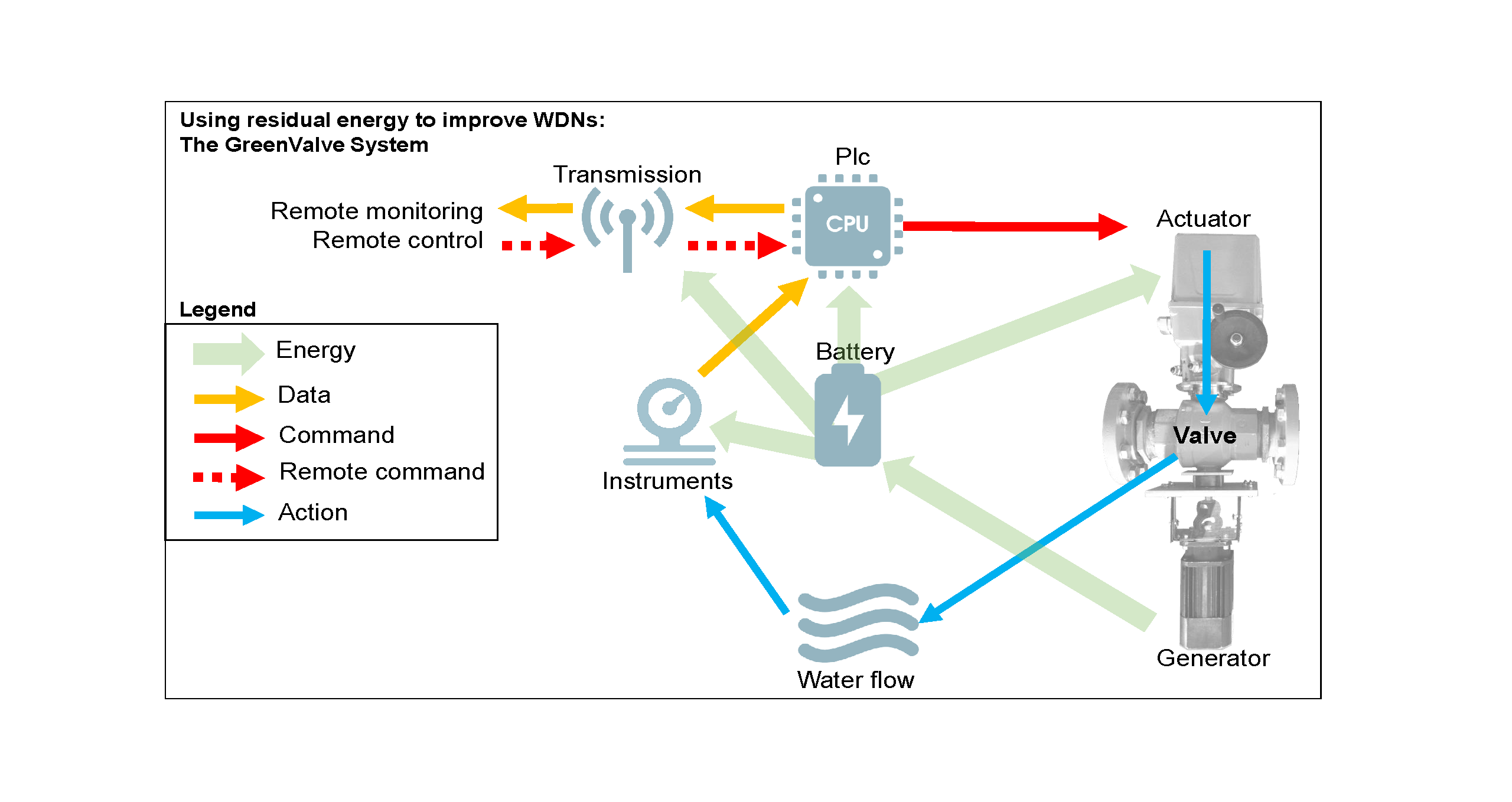
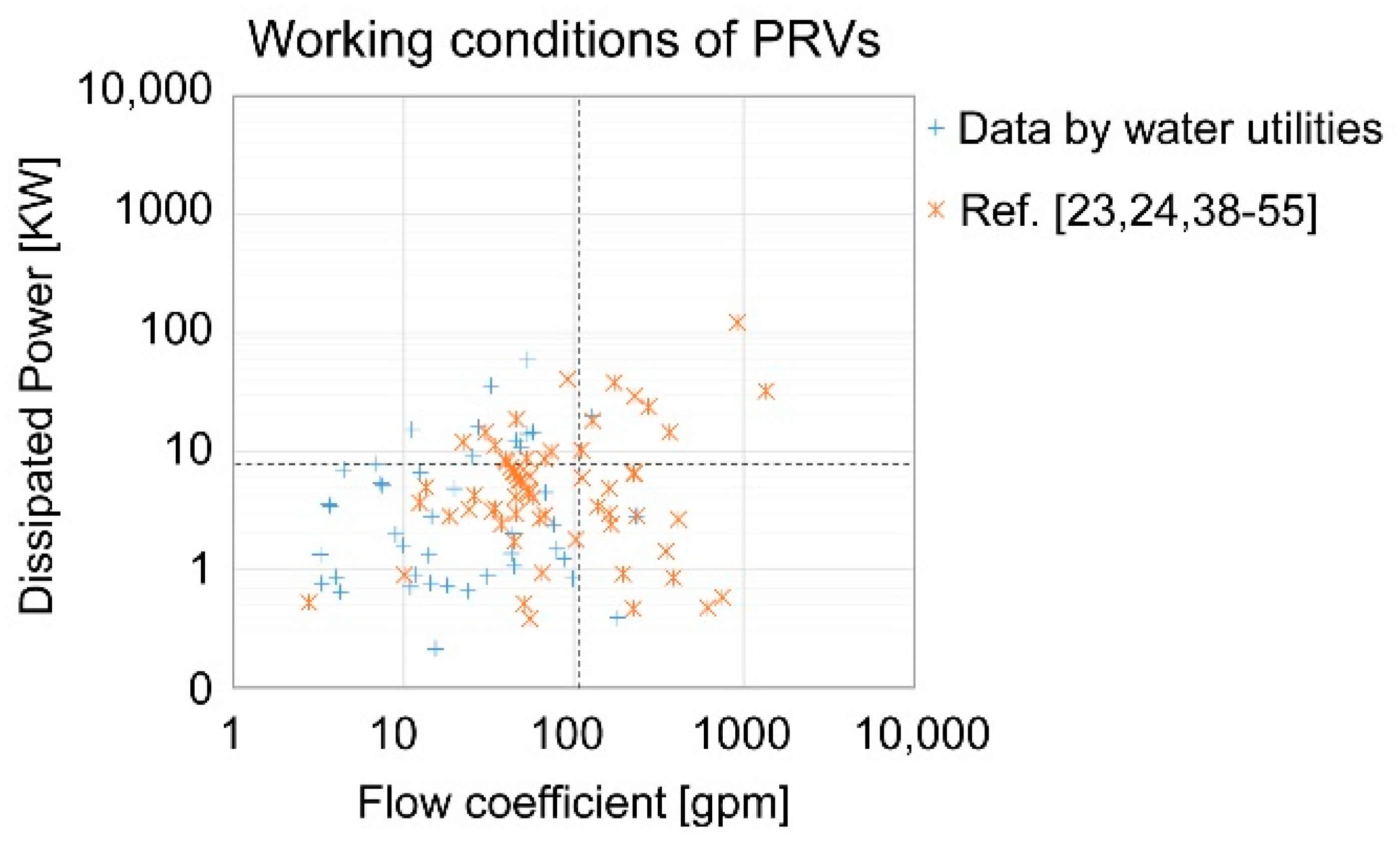
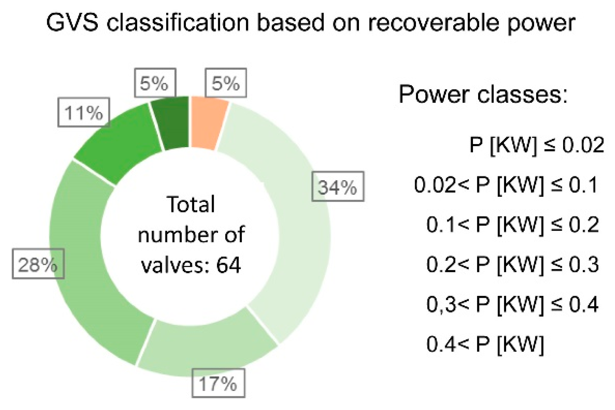
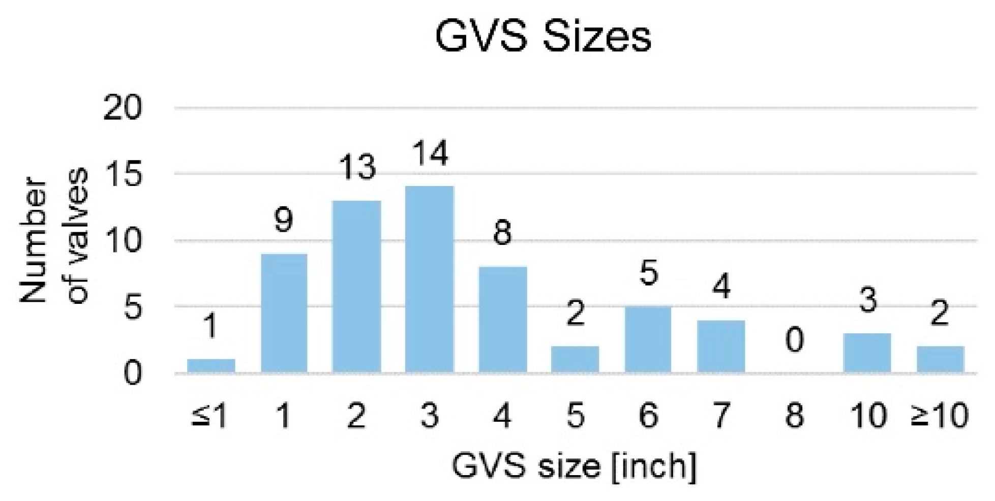
2. Data Set Classification and Analysis

The hydraulic data about the regulation made by PRVs that are primarily installed at the entrance of DMAs are collected in the following. The series of data used in the present study is shown with their source in Appendix A. The dissipated power and flow coefficient are calculated on the basis of the average flow rate and pressure drop of

Table A1. Working conditions of the pressure-reducing valve (PRV) considered in the study.

	Ref.	Location	n°	Kind of Application	Type of Data	Q (L/s)	ΔP (bar)	PD (KW)
Data from bibliography	[23]	Benevento Municipality DMA Santa Colomba	1	PRV	avg	26.9	0.34	0.91
	[24]	Northern Italy	2	RTC	avg	58.6	1.17	6.55
	[38]	York, North of Toronto, Ontario, Canada	3	PRV	avg	98.5	0.99	2.66
		York, North of Toronto, Ontario, Canada	4	PRV	avg	73.8	0.78	1.43
	[39]	Durban, South Africa	5	PRV	avg	390.7	3.17	121.1
	[40]	El Dorado Irrigation District, Ca, USA	6	PRV	avg	15.1	7.92	11.9
	[41]	Halifax, Canada	7	PRV	avg	53.6	1.90	2.95
	[42]	Coviolo, Italy	8	PRV	avg	3.67	2.30	0.90
	[43]	Razgrad, Bulgaria	9	PRV	avg	8.75	0.44	0.38
	[44]	Skopje, Macedonia	10	PRV	avg	44.3	1.30	4.87
	[45]	Naples (EAST), Italy	11	PRV	avg model	323.0	1.00	32.21
	[46]	UK	12	PRV	avg	12.14	3.76	4.24
		UK	13	PRV	avg	1.34	4.04	0.53
		UK	14	PRV	avg	9.19	0.56	0.52
	[47]	Rural area in northern Germany	15	PRV	avg	6.89	5.36	3.65
	[48]	Philadephia, USA	16	PRV	avg model	33.6	0.71	2.40
	[49]	Selangor, Malaysia	17	PRV	avg	18.9	1.57	2.68
		Selangor, Malaysia	18	PRV	avg	22.6	0.84	1.79
		Selangor, Malaysia	19	PRV	avg	14.5	0.86	0.93
	[50]	n.d.	20	PRV	avg model	103.6	1.39	14.4
	[51]	n.d.	21	PRV	avg model	17.0	2.43	4.12
		n.d.	22	PRV	avg model	101.9	2.39	23.6
	[52]	n.d	23	PRV	avg model	36.0	1.80	5.93
		n.d	24	PRV	avg model	47.4	0.71	2.83
	[53]	Central Arava Valley, Israel	25	PRV	avg model	23.3	0.04	0.09
		Central Arava Valley, Israel	26	PRV	avg model	15.3	1.94	2.96
		Central Arava Valley, Israel	27	PRV	avg model	58.1	6.93	40.3
		Central Arava Valley, Israel	28	PRV	avg model	31.4	3.16	9.92
		Central Arava Valley, Israel	29	PRV	avg model	33.3	1.02	3.40
		Central Arava Valley, Israel	30	PRV	avg model	12.5	1.94	2.42
		Central Arava Valley, Israel	31	PRV	avg model	41.7	2.45	10.2
		Central Arava Valley, Israel	32	PRV	avg model	41.7	0.20	0.85
		Central Arava Valley, Israel	33	PRV	avg model	46.9	0.10	0.48
		Central Arava Valley, Israel	34	PRV	avg model	86.7	4.39	38.0
		Central Arava Valley, Israel	35	PRV	avg model	57.2	1.12	6.42
		Central Arava Valley, Israel	36	PRV	avg model	57.2	0.10	0.58
	[54]	Pato Branco, Brasil	37	PRV	avg	19.6	3.13	6.15
		Pato Branco, Brasil	38	PRV	avg	23.8	0.20	0.47
		Pato Branco, Brasil	39	PRV	avg	12.6	1.37	1.72
		Pato Branco, Brasil	40	PRV	avg	19.6	2.84	5.58
		Pato Branco, Brasil	41	PRV	avg	19.6	5.68	11.2
		Pato Branco, Brasil	42	PRV	avg	19.7	1.47	2.89
		Pato Branco, Brasil	43	PRV	avg	8.1	6.17	4.97
		Pato Branco, Brasil	44	PRV	avg	19.6	2.06	4.04
		Pato Branco, Brasil	45	PRV	avg	19.6	2.25	4.43
		Pato Branco, Brasil	46	PRV	avg	19.6	3.33	6.54
		Pato Branco, Brasil	47	PRV	avg	28.3	6.56	18.6
		Pato Branco, Brasil	48	PRV	avg	19.6	2.94	5.77
		Pato Branco, Brasil	49	PRV	avg	19.6	3.43	6.73
		Pato Branco, Brasil	50	PRV	avg	19.6	4.31	8.47
		Pato Branco, Brasil	51	PRV	avg	19.6	7.35	14.4
		Pato Branco, Brasil	52	PRV	avg	19.7	2.35	4.62
		Pato Branco, Brasil	53	PRV	avg	28.3	3.04	8.59
		Pato Branco, Brasil	54	PRV	avg	95.1	3.04	28.9
		Pato Branco, Brasil	55	PRV	avg	19.6	4.11	8.08
		Pato Branco, Brasil	56	PRV	avg	19.7	3.72	7.31
	[55]	Kozani, Greece	57	PRV	avg model	22.1	2.77	6.11
		Kozani, Greece	58	PRV	avg model	55.8	3.25	18.1
		Kozani, Greece	59	PRV	avg model	12.6	2.48	3.13
		Kozani, Greece	60	PRV	avg model	24.1	3.59	8.65
		Kozani, Greece	61	PRV	avg model	13.1	2.51	3.29
		Kozani, Greece	62	PRV	avg model	10.2	3.11	3.18
		Kozani, Greece	63	PRV	avg model	8.26	3.40	2.81
Data by water utilities		Switzerland	64	PRV	avg	2.0	4.31	0.86
		Romania	65	PRV	avg	1.25	0.40	0.05
		Romania	66	PRV	avg	19.4	0.20	0.39
		Belluno, Italy	67	PRV	avg	11.3	1.21	1.37
		Piemonte, Italy	68	PRV	avg model	4.50	3.56	1.60
		Piemonte, Italy	69	PRV	avg model	2.00	6.65	1.33
		Emilia Romagna, Italy	70	PRV	avg	4.14	2.18	0.90
		Emilia Romagna, Italy	71	PRV	avg	13.0	1.54	2.01
		Emilia Romagna, Italy	72	PRV	avg	5.30	2.50	1.33
		Emilia Romagna, Italy	73	PRV	avg	1.88	3.42	0.64
		Emilia Romagna, Italy	74	PRV	avg	1.68	4.52	0.76
		Emilia Romagna, Italy	75	PRV	avg	10.3	4.69	4.83
		Emilia Romagna, Italy	76	PRV	avg	7.88	1.11	0.87
		Emilia Romagna, Italy	77	PRV	avg	5.15	1.42	0.73
		Lombardia, Italy	78	PRV	avg	27.9	12.8	35.5
		Lombardia, Italy	79	PRV	avg	45.8	12.8	58.4
		Lombardia, Italy	80	PRV	avg	4.30	16.2	6.95
		Lombardia, Italy	81	PRV	avg	3.67	1.96	0.72
		Lombardia, Italy	82	PRV	avg	22.8	1.96	4.47
		Lombardia, Italy	83	PRV	avg	24.6	5.00	12.3
		Lombardia, Italy	84	PRV	avg	8.40	7.84	6.59
		Lombardia, Italy	85	PRV	avg	28.4	4.90	13.9
		Lombardia, Italy	86	PRV	avg	10.3	14.7	15.1
		Lombardia, Italy	87	PRV	avg	24.5	4.41	10.8
		Lombardia, Italy	88	PRV	avg	19.0	8.40	16.0
		Lombardia, Italy	89	PRV	avg	4.50	1.70	0.77
		Lombardia, Italy	90	PRV	avg	4.50	4.40	1.98
		Lombardia, Italy	91	PRV	avg	7.00	4.00	2.80
		Lombardia, Italy	92	PRV	avg	6.00	13.0	7.80
		Lombardia, Italy	93	PRV	avg	6.00	1.10	0.66
		Lombardia, Italy	94	PRV	avg	20.0	1.20	2.40
		Lombardia, Italy	95	PRV	avg	30.1	4.77	14.4
		Lombardia, Italy	96	PRV	avg	57.1	3.44	19.7
		Lombardia, Italy	97	PRV	avg	16.8	0.50	0.84
		Lombardia, Italy	98	PRV	avg	10.7	1.00	1.07
		Lombardia, Italy	99	PRV	avg	44.3	0.6	2.81
		Lombardia, Italy	100	PRV	avg	3.08	0.69	0.21
		Lombardia, Italy	101	PRV	project	5.50	9.30	5.12
		Lombardia, Italy	102	PRV	project	5.50	9.75	5.36
		Lombardia, Italy	103	PRV	project	3.00	11.5	3.44
		Lombardia, Italy	104	PRV	project	3.00	11.9	3.57
		Lombardia, Italy	105	PRV	project	17.6	0.70	1.23
		Lombardia, Italy	106	PRV	project	17.6	0.85	1.50
		Lombardia, Italy	107	PRV	project	15.0	6.00	9.00

. The flow coefficient CV is a coefficient widely used in the field of valves. It relates discharge and pressure drop, as defined in the following formula from [31]:

$$CV=\frac{Q}{N_1}\sqrt{\frac{{\rho }_1/{\rho }_0}{\Delta P}}$$

(1)

where ${\rho }_1$ (Kg m⁻³) is the density of the used fluid, ${\rho }_0$ (Kg m⁻³) is the reference density in standard condition (water at 15 °C and 1 atm), and ∆p is the difference between the pressure P1 measured upstream of the valve and P2 measured downstream of the valve. N₁ represents a constant that depends on the unit used for Q and ∆p. In the following, N₁ is equal to 0.865 with Q expressed in m³ h⁻¹ and ∆p in bar. Following these specifications, the flow coefficient is commonly called CV (gpm).

An index commonly used to scale the capacity of geometrically similar control valves is the capacity index, defined as

$$C{V}_D=CV/D^2$$

(2)

where $D$ (in) is the diameter of the valve.

The power $P_D$ dissipated by each PRV is calculated as follows:

$$P_D=Q·\mathsf{\Delta }P$$

(3)

where $Q$ is the average flow rate and $\mathsf{\Delta }P$ the average pressure drop through a single PRV. They are expressed, respectively, in m³ s⁻¹ and Pa, in order to obtain the power in W.

Naturally, the daily oscillation of demand can affect the results, but with a preliminary analysis, it can be neglected without losing significance [32].

Figure 1 shows the power $P_D$ dissipated through each valve of Table A1, as a function of the working flow coefficient CV. Dotted lines in Figure 1 represent the average flow coefficient and average dissipated power calculated, considering all the sites presented in Table A1. The total dissipated power, calculated by summing the power dissipated by each PRV, is 856.7 KW, with an average of 7.86 KW. The data indicated as “by water utilities” have been provided by water utility managers to the authors. The size of the valves of Table A1 is not available, but it can be approximately deduced by considering the capacity index (CV_max/D²) of common pressure-reducing valves [33,34,35,36,37], which ranges between 10.75 and 12.5, with an average of 11.25. Thus the calculated flow coefficients indicate that the size of the valves of Figure 1 ranges between 1.5 to 14 inches and that 3 and 4 inches are the most common sizes.

In Figure 2, the PRVs are grouped on the basis of the dissipated power. Where data are available, the dissipated power is based on monitoring measurements. In other cases, it is calculated by means of average flow rates and pressure drops through the valve.

Figure 2a shows that there are a large number of PRVs that dissipate energy below 5 KW, i.e., more than half of the total. It can be clearly seen in Figure 2b that most of the energy is dissipated by the classes over 10 KW, representing 68% of the total amount of dissipated power.

Thanks to this data, some considerations can be made. The first is that it is possible to recover most of the power dissipated in the regulation process by introducing energy recovery systems, such as PAT or cross-flow turbine, in only the most powerful sites. Figure 2 proves that replacing PRVs that dissipate more than 10 KW with energy recovery devices can potentially recover 68% of the total power dissipated. The second consideration is that 60% of the valves dissipate power below 5 KW, cumulating in only 15% of the total amount of dissipated power. The results are in agreement with the study presented in [32], where, on a total amount of 95 considered sites in aqueducts placed in Ireland and UK, 56% of the cases showed dissipated power below 5 KW.

In the following, a preliminary economic analysis is shown. The analysis evaluates which are the PRVs that may be economically promising for energy production by substitution of the PRV with an energy recovery device. The other PRVs are instead highlighted as possible application sites for the GVS.

In Figure 3a, the payback periods of all the cases of Table A1 are shown. A specific cost of the energy recovery plant of 3700 €/KW in the best scenario, and of 7400 €/KW in the worst [56], is used in the calculation of investment cost $C_i$. The specific cost expresses the relation between the initial investment cost and the nominal power of the plant. The payback period is calculated as the minimum period required to recoup the funds expended in the investment. The calculations have been made considering a depreciation rate $r_D$ to be calculated as follows:

$$r_D=\frac{r{\left(1+r\right)}^t}{{\left(1+r\right)}^t-1}$$

(4)

where r is the discount rate that is considered equal to 0.05. In the calculation, an investment period t of ten years is used, which can be considered a threshold for investment profitability by water utilities. The average European price of electricity for consumer $C_e$ (equal to 0.18 €/KWh) is considered equal to the selling price because the energy is considered to be consumed onsite. The annual net income (ANI) is calculated as

$$\mathrm{ANI}=C_e{E}_R-r_D\left(C_i\right)-C_m$$

(5)

where $C_m$ is the maintenance cost that is calculated as 1600 €/year [57]; it is considered a conservative estimate valid for the range of power. To calculate the annual recovered energy $E_R$, a constant efficiency ${\eta }_T$ of 0.65 [32] is used in the following equation:

$$E_R={\eta }_T{P}_D·\left(365·24\right)$$

(6)

Figure 3a shows that the payback period is below 10 years only for installed powers above 2.95 KW, considering the series relative to the minimum specific investment cost of 3700 €/KW. Figure 3b shows a positive ANI—and, thus, a feasible investment—is obtained only for cases with installed power above 2.95 KW. The results change dramatically if the maximum specific investment cost is considered. In Figure 3a, the blue series shows that the minimum installed power to obtain a payback period below 10 years is 25 KW. The same result can be seen, in terms of ANI, in the blue series in Figure 3b. The specific investment cost is expected to increase when the size of the plant decreases due to the existence of some fixed costs, such as civil works and maintenance. The impact of these fixed costs decreases with the increase of installed power [58]. Thus the blue series is more accurate for low power plants, and the green series is more accurate for high power plants. It is possible to say that the two series identify a band to which the effective results belong.

This preliminary economic analysis shows that the sites, where PRVs dissipate power below 2.95 KW, are economically unfeasible for energy production purposes. It is worth saying that the value of 2.95 KW increases quickly when increasing the specific investment cost, but, unfortunately, cannot be precisely evaluated without accurate knowledge of the installation site. The study performed in [59] on the application of energy-recovery devices in several aqueducts sites found that all the sites with potential power below 10 KW resulted in being unfeasible from an economic point of view.

Where standard energy recovery devices are not profitable for producing energy, the GVS is a new possible solution for residual energy recovery and the optimization of the water network. In the following, GVSs will be sized, and the applicability of the system will be verified for sites with potential power below 5 KW, which can be considered a reasonable threshold for energy production. The PRVs in this power class represent a significant part of the database, namely, 60% of the total or 64 PRVs.

Limitations

The study is based on average data (see Appendix A). This approach represents a limitation because it neglects the daily and seasonal variation of demand. Following demand, the working conditions of pressure and flow rate of single PRVs can undergo dramatic variations during the day and the seasons. A sufficient history of the data was not available to make considerations about this point, but in [32], the difference between the yearly energy recovered, calculated on the basis of average values, and quarter-of-hour-based values were comparable, even though average values generally overestimate the energy recovered.

The energy selling price $C_e$ is considered constant and equal to the average European price of electricity for consumers. Thus, the considered selling price can bring an underestimation of the payback period and an overestimation of the ANI, at least for large power plants that most likely sell energy at a lower price.

The calculation of the effective specific investment cost of the plant should take into account many factors depending on the local conditions of the specific case. Two specific investment costs are considered to address the problem. The first one (3700 €/KW), considered as the best scenario, is characteristic for high power plants that usually have a low specific cost [56]. The other (7400 €/KW), considered as the worst scenario, is characteristic for low power plants that usually have a high specific cost. In this way, an interval of confidence is created in which the effective specific cost of the plant most likely belongs. Considering the best scenario, the calculated payback period is underestimated and the ANI overestimated.

The scope of the performed economic analysis is to find a power threshold below which the application of standard energy recovery devices is most likely economically unfeasible. The GVS is presented as an alternative solution to substitute PRVs in these cases. The possible underestimation of this power threshold, due to the aforementioned limitations, increases the probability that the range of applicability of the GVS is larger than the one found. The power threshold considered was increased from 2.95 to 5 KW to take into account this probability.

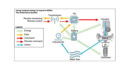
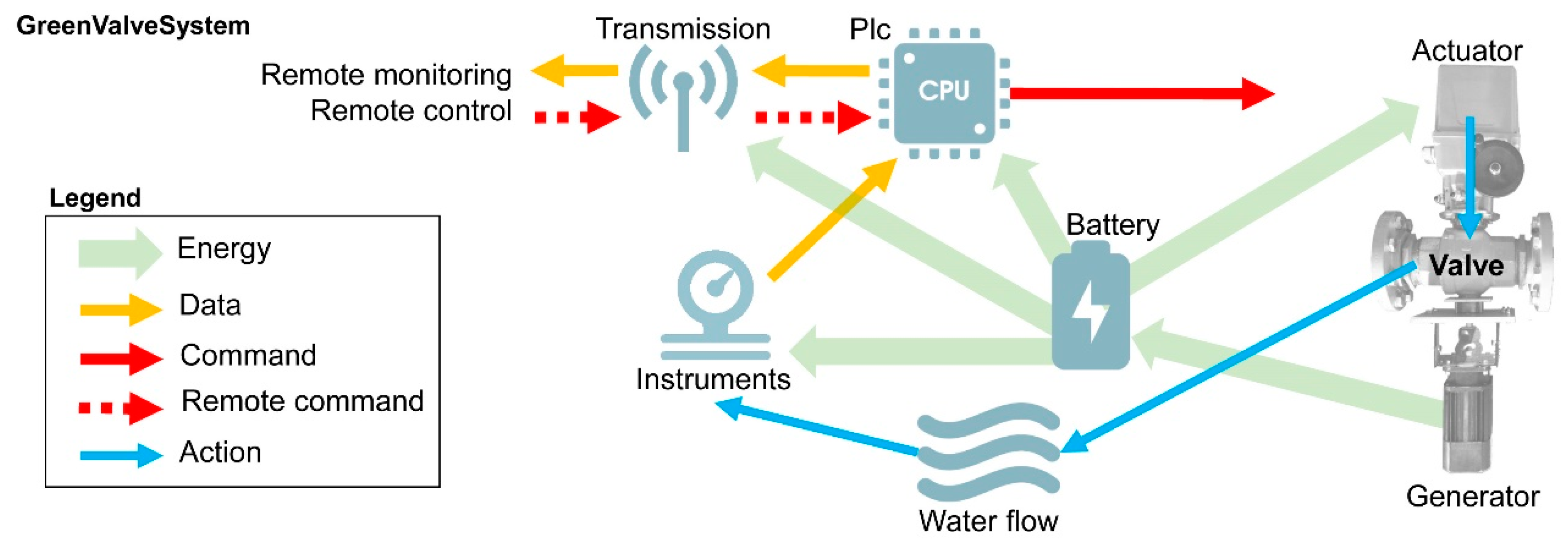
3. GreenValve System (GVS)

The GreenValve system (GVS) is an innovative control valve, based on a patent by the Politecnico di Milano [60], designed to harvest energy while controlling the flow. A detailed description of the hydraulic, mechanical parts of the GVS can be found in [30].

It was developed to replace PRVs without changing the water network operating conditions and with no need to install further components in the network. This last feature represents an important advantage since it lowers the installation costs and the difficulties, such as the necessity of flow meter installation.

The GVS is composed of the mechanic hydraulic main part, the GreenValve (GV), and other electro-mechanic components that create the GreenValve system (GVS). The GreenValve (GV) is structurally made up of a ball valve and a turbine, whose impeller is fixed inside the body of the ball. The axes, around which the ball and the impeller rotate, coincide. This choice comes from the desire to create a control valve that requires only simple constructive changes of a common ball valve. The axis is linked to a shaft that can transfer the torque of the impeller to an energy transformer.

The electrical energy recovered is used to feed a battery that powers the entire system. The basic system layout is composed of the main body GV, with two integrated pressure transducers, an electrical actuator, a generator, and a control box that contains a controller, a battery pack, and a communication system. The system is able to collect and transmit data through 3G networks to a cloud database available for queries by users. The data transmitted are the GVS control parameters and the monitoring data such as the upstream and downstream pressures, the flow rate, as well as any data of further instruments added to the base configuration.

The power recovered allows real-time monitoring and real-time actions on the valve, enabling new strategies for pressure management and network optimization without any limitations, owing to the presence of the electrical net. A functioning scheme of the system can be seen in Figure 4. The minimum power necessary to feed the system has been calculated to be 15 W for a 3-inch valve, considering data transmission with 1 Hz frequency and 30 movements per hour, each lasting 5 s. The consumption has been calculated on the basis of laboratory tests on a 3-inch valve. Naturally, this power increases with the size of the valve because the power size of the actuator will increase as well. However, this scarcely influences energy consumption as the hourly operating time of the actuator is limited.

The controller is programmed with preinstalled logics that are able to reproduce the principal functions of common PRVs, such as pressure sustain or pressure reduction. In any case, the controller can be programmed to achieve the requirements of the site or to implement remote pressure control. In fact, thanks to the electronics available on the GVS, it is possible to remotely update the control parameters, for example, the target pressure or the programmed logic itself. The GVS can be updated on the basis of the data acquired by the system itself, creating a framework to enable the development of new pressure control strategies not viable with other devices.

Other specific features include the possibility of regulating the velocity of actuation to achieve the needs of the plant, such as fast opening or the control of low flow rates, as well as the possibility of programming specific alarms based on the monitored quantities or their combination.

For a fixed valve opening, the rotational velocity of the impeller can change without affecting the flow coefficient of the valve. This means that the control process and the energy-harvesting process are independent of each other. As a consequence, if the impeller stops due to breakdowns, the valve will continue throttling the flow unconditionally.

Thanks to an algorithm installed on the controller and developed through specific laboratory characterization, the GVS is able to deliver flow rate measures. In this way, the installation of a flow meter can be avoided, simplifying the installation and further reducing the costs.

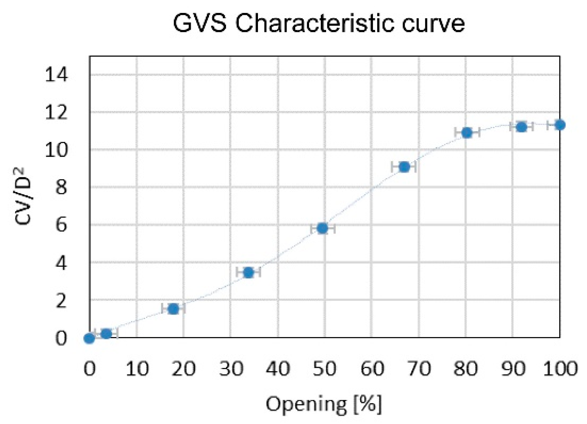
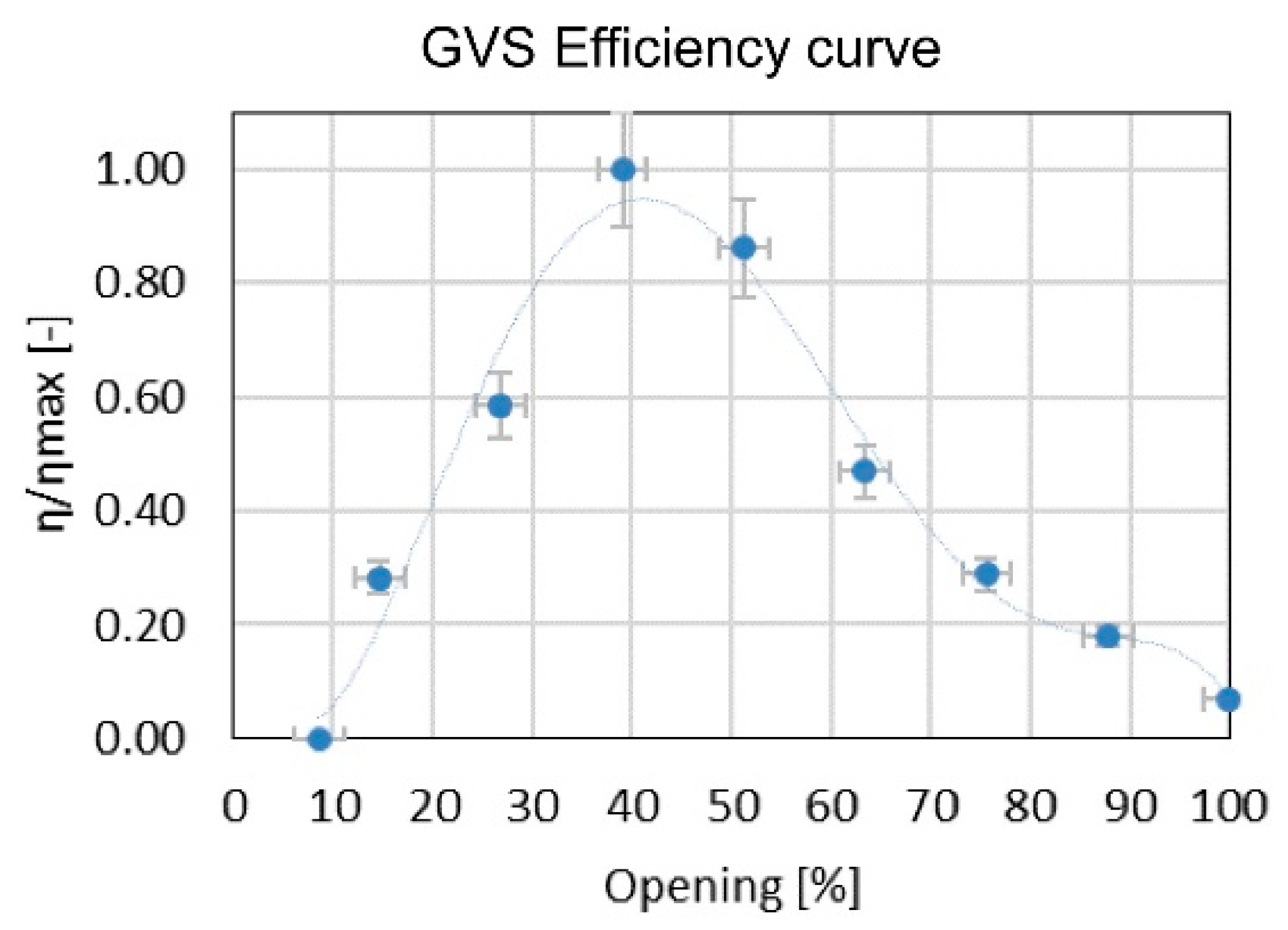
GVS Sizing Procedure

The GVS sizing procedure is based on the flow coefficient (CV) required for the application.

To guarantee sufficient overflow capacity with respect to average working conditions, the valve is sized to work at 40% of the capacity. It is worth noting that the minimum flow rate can also become critical and must be considered to evaluate the reliability of the installation. Sometimes, standard PRV installation provides for the use of a smaller bypass to increase the low flow capability [38]. In the case of the GVS, the problem of low flow is addressed by a specific control mode of the system.

Figure 5 reports the capacity index, defined in Equation (2), as a function of valve opening, resulting from experimental tests performed in the “control valve section” of the Hydraulic Laboratory “G. Fantoli” at the Politecnico di Milano. In the present paper, only the results of the experimental campaign that are necessary for the sizing procedure of the GVS are introduced.

The harvested power is calculated as a percentage of the power dissipated by the valve:

$$P_H={\eta }_h{P}_D$$

(7)

where $P_H$ (W) is the power recovered by the GV, ${\eta }_h$ is the efficiency of the harvesting process, and $P_D$ (W) is the dissipated power defined in Equation (3).

Figure 6 shows the relation between the normalized efficiency of mechanical energy recovery $\eta /{\eta }_{max}$ and the opening of the valve. The highest efficiency corresponds to an opening degree of about 40%, with a measured maximum mechanical efficiency ${\eta }_{max}$ of 14.5%. The experimental analysis has been performed on a 3-inch prototype. The scale effect on efficiency is neglected in this sizing procedure.

Knowing the average flow coefficient required by the site (calculated by PRV average working conditions of Table A1), the required GVS diameter can be calculated by using Equation (2). The efficiency should then be reduced to take into account the loss due to energy transformation caused by the generator. In this case, a prudential efficiency ${\eta }_g$ equal to 0.6 is used to take into account the possible large variability of the conditions. The overall efficiency can then be estimated as

$${\eta }_h={\eta }_g\eta$$

(8)

Finally, the power recovered can be calculated by introducing to Equation (7) the overall efficiency ${\eta }_h$. More information and details about the experimental campaign behind some aspects of the GVS are provided in [30].

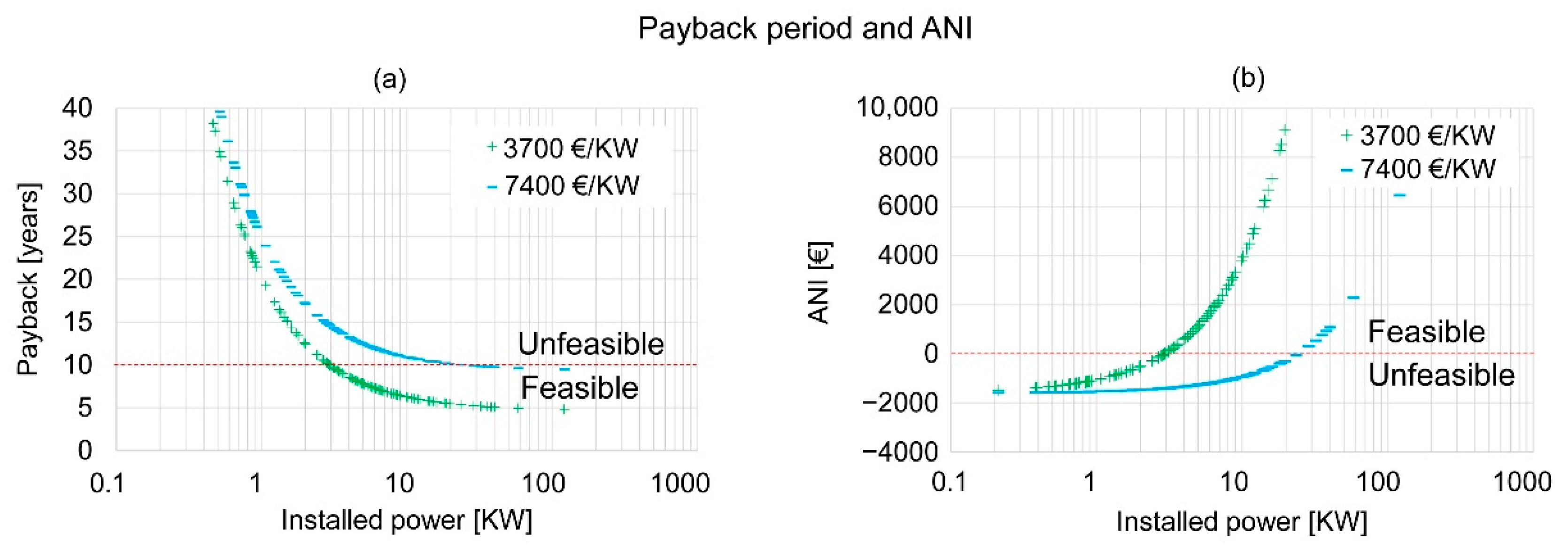
4. GVS Applicability to Dataset

Section 2 highlights that the PRVs that dissipate power below 5 KW can represent promising GVS installation sites. The installation can enhance the energy efficiency of WDNs by exploiting the residual energy. The energy recovered by the GVS is used directly on site for the functioning of the system and, if a surplus is available, for other useful local services. Hence the energy, even if it is a low amount, gains value because it enables new functionalities. It must be noted that in the reported cases, the GVS is proposed as an alternative to standard control devices, which are installed on the site for the good functioning of the plant.

Through the procedure described in Section 3, the potential recovered energy for each site of Table A1 below 5 KW is calculated. The sites that show recovered power below 20 W, which is the minimum power necessary to feed the GVS system, are discarded. With these conditions, 61 potential PRVs can be substituted by the GVS, representing 95% of the considered PRVs, with an average power of 179 W. In Figure 7, the results of the calculations are shown, in particular, the sized GVSs are divided into power classes, showing that just 5% (in orange) cannot be considered for GVS application.

Figure 8 reports the diameters of the sized GVSs and the number of valves for each size. The most common size range is between 1 and 4 inches.

Every GVS considered in Figure 8 can harvest an average power greater than 20 W, meaning that the recoverable power may be used to feed the automatic control, the monitoring sensor system, the data transmission system, and the battery. Depending on the potential of the site, the energy stored may be reused by water utilities to satisfy whatever needs they may have while managing WDNs. It has been demonstrated that the GVS can be used in place of a large part of the PRVs presented in the study, which are mainly valves used at the entrance of DMAs. The use of GVSs at the entrance of all the DMAs of a network can create a framework for the management of the WDN that is promising in terms of efficiency improvement. In fact, real-time management allows a dynamic answer of the system to sudden demand scenarios that could potentially put static DMA patterns in crisis. The DMAs themselves can be transformed into a more flexible scheme that can change its pattern depending on demand requirements, increasing plant resilience [61]. The study of such management methods can be the subject of future works.

The GVS is designed to have sizes very similar to common PRVs, a feature that considerably simplifies the substitution and can reduce the costs of installation compared to a standard energy recovery system. In fact, a standard energy recovery system requires auxiliary operations, such as the installation of flowmeters and pressure transducers, electric grid connection, and a control system like the one described in [29]. GVS is an integrated, simple-to-install, stand-alone system that can be substituted for common control valves without the necessity of further devices.

5. Conclusions

The evaluation of the applicability of the GVS based on a wide dataset of PRV working conditions is provided. The study, based on average data and on the minimum energy required by the system, shows a clear view of the potential installation of the GVS. The GVS permits the control of flows (reducing pressure and throttling discharge) while harvesting residual energy.

More than one hundred PRVs were taken into account for the study. Firstly, an economic calculation was made on each PRV to evaluate the minimum amount of potential power that must be available to achieve a feasible substitution of the PRV with a standard energy recovery device. The minimum amount of power was between 2.95 and 25 KW, depending on the specific installation cost used for the calculation. It has been deemed that a critical threshold could be 5 KW. Then, the sites that show a dissipated power below 5 KW were considered for potential substitution of existent PRVs with the GVS. It was verified that the technology is applicable in 95% of the cases. The recovered power is sufficient to allow the stand-alone functioning of every GVS and to feed the monitoring systems that can be used to control the hydraulic conditions of the WDN.

This study highlights the wide applicability of the GVS within WDNs. Moreover, this technology can be applied in a range of conditions where the production of energy with common energy recovery devices is otherwise inconvenient. The economic feasibility of the GVS should take into account not only the amount of energy produced, but also the advantages that a completely stand-alone system can offer to real-time management of WDNs.

GVS can be considered an effective tool to improve the frameworks of smart water distribution systems. It is known [61] that the creation of DMAs can improve the performances of the water network; however, it significantly reduces the resilience of the system by introducing some “static” partitions in the network. The use of GVS instead of simple valves, commonly used for the creation of DMAs, can bring a considerable increase of the plant resilience since the valve can be remotely managed, enabling new dynamic strategies for pressure management and network optimization.

References

1. Abd Rahman, N.; Muhammad, N.S.; Wan Mohtar, W.H.M. Evolution of research on water leakage control strategies: Where are we now? Urban Water J. 2018, 15, 812–826. [Google Scholar] [CrossRef]
2. Xu, Q.; Liu, R.; Chen, Q.; Li, R. Review on water leakage control in distribution networks and the associated environmental benefits. J. Environ. Sci. 2014, 26, 955–961. [Google Scholar] [CrossRef]
3. Giugni, M.; Fontana, N.; Ranucci, A. Optimal location of PRVs and turbines in water distribution systems. J. Water Resour. Plan. Manag. 2014, 140, 06014004. [Google Scholar] [CrossRef]
4. Creaco, E.; Pezzinga, G. Comparison of algorithms for the optimal location of control valves for leakage reduction in WDNs. Water 2018, 10, 466. [Google Scholar] [CrossRef] [Green Version]
5. Covelli, C.; Cozzolino, L.; Cimorelli, L.; Della Morte, R.; Pianese, D. Optimal Location and Setting of PRVs in WDS for Leakage Minimization. Water Resour. Manag. 2016, 30, 1803–1817. [Google Scholar] [CrossRef] [Green Version]
6. Reis, L.F.R.; Porto, R.M.; Chaudhry, F.H. Optimal location of control valves in pipe networks by genbetic algorithms. J. Water Resour. Plan. Manag. 1997, 123, 317–326. [Google Scholar] [CrossRef]
7. Tucciarelli, T.; Criminisi, A.; Termini, D. Leak analysis in pipeline system by means of optimal valve regulation. J. Hydraul. Eng. 1999, 125, 277–285. [Google Scholar] [CrossRef]
8. Pezzinga, G.; Pititto, G. Combined optimization of pipes and control valves in water distribution networks. J. Hydraul. Res. 2005, 43, 668–677. [Google Scholar] [CrossRef]
9. Araujo, L.S.; Ramos, H.; Coelho, S.T. Pressure control for leakage minimisation in water distribution systems management. Water Resour. Manag. 2006, 20, 133–149. [Google Scholar] [CrossRef]
10. Nicolini, M.; Zovato, L. Optimal location and control of pressure reducing valves in water networks. J. Water Resour. Plan. Manag. 2009, 135, 13–22. [Google Scholar] [CrossRef]
11. Jowitt, B.P.W.; Xu, C. Optimal valve control in water distribution networks. J. Water Resour. Plan. Manag. 1990, 116, 455–472. [Google Scholar] [CrossRef]
12. Vairavamoorthy, K.; Lumbers, J. Leakage reduction in water distribution systems: Optimal valve control. J. Hydraul. Eng. 1998, 124, 1146–1154. [Google Scholar] [CrossRef]
13. Awad, H.; Kapelan, Z.; Savic, D. Analysis of pressure management economics in water distribution systems. In Proceedings of the 10th Annual Water Distribution Systems Analysis Conference (WDSA2008), Kruger National Park, South Africa, 17–20 August 2008. [Google Scholar]
14. Giustolisi, O.; Savic, D.; Kapelan, Z. Pressure-driven demand and leakage simulation for water distribution network. J. Hydraul. Eng. 2008, 134, 625–635. [Google Scholar] [CrossRef] [Green Version]
15. Raei, E.; Nikoo, M.R.; Pourshahabi, S.; Sadegh, M. Optimal joint deployment of flow and pressure sensors for leak identification in water distribution networks. Urban Water J. 2018, 15, 837–846. [Google Scholar] [CrossRef]
16. Alvisi, S.; Franchini, M. A procedure for the design of district metered areas in water distribution systems. Procedia Eng. 2014, 70, 41–50. [Google Scholar] [CrossRef] [Green Version]
17. Giustolisi, O.; Ridolfi, L. New modularity-based approach to segmentation of water distribution networks. J. Hydraul. Eng. 2014, 140, 04014049. [Google Scholar] [CrossRef]
18. Ferrari, G.; Savic, D. Economic performance of DMAs in water distribution systems. Procedia Eng. 2015, 119, 189–195. [Google Scholar] [CrossRef] [Green Version]
19. Simone, A.; Lucelli, D.; Berardi, L.; Giustolisi, O. Modularity Index for optimal sensor placement in WDNs. In Advances in Hydroinformatics; Philippe, G., Jean, C., Guy, C., Eds.; Springer: Singapore, 2018; pp. 433–446. ISBN 9789811072178. [Google Scholar]
20. Page, P.R.; Abu-Mahfouz, A.M.; Yoyo, S. Parameter-Less remote real-time control for the adjustment of pressure in water distribution systems. J. Water Resour. Plan. Manag. 2017, 143, 04017050. [Google Scholar] [CrossRef] [Green Version]
21. Campisano, A.; Modica, C.; Reitano, S.; Ugarelli, R.; Bagherian, S. Field-oriented methodology for real-time pressure control to reduce leakage in water distribution networks. J. Water Resour. Plan. Manag. 2016, 142, 04016057. [Google Scholar] [CrossRef]
22. Fontana, N.; Giugni, M.; Glielmo, L.; Marini, G.; Verrilli, F. Real-Time control of a PRV in water distribution networks for pressure regulation: Theoretical framework and laboratory experiments. J. Water Resour. Plan. Manag. 2017, 144, 04017075. [Google Scholar] [CrossRef]
23. Fontana, N.; Giugni, M.; Glielmo, L.; Marini, G.; Zollo, R. Real-time control of pressure for leakage reduction in water distribution network: Field experiments. J. Water Resour. Plan. Manag. 2018, 144, 04017096. [Google Scholar] [CrossRef]
24. Page, P.; Creaco, E. Comparison of flow-dependent controllers for remote real-time pressure control in a water distribution system with stochastic consumption. Water 2019, 11, 422. [Google Scholar] [CrossRef] [Green Version]
25. Sammartano, V.; Aricò, C.; Carravetta, A.; Fecarotta, O.; Tucciarelli, T. Banki-Michell optimal design by computational fluid dynamics testing and hydrodynamic analysis. Energies 2013, 6, 2362–2385. [Google Scholar] [CrossRef]
26. Sinagra, M.; Sammartano, V.; Aricò, C.; Collura, A.; Tucciarelli, T. Cross-Flow turbine design for variable operating conditions. Procedia Eng. 2014, 70, 1539–1548. [Google Scholar] [CrossRef] [Green Version]
27. Chapallaz, J.M.; Eichenberg, P.; Fisher, G. Manual on Pumps Used As Turbines. In Harnessing Water Power on Small Scale; Vieweg: Braunschweig, Germany, 1992; Volume 11, p. 221. [Google Scholar]
28. Carravetta, A.; del Giudice, G.; Fecarotta, O.; Ramos, H.M. PAT design strategy for energy recovery in water distribution networks by electrical regulation. Energies 2013, 6, 411–424. [Google Scholar] [CrossRef] [Green Version]
29. Carravetta, A.; Fecarotta, O.; Ramos, H.M. A new low-cost installation scheme of PATs for pico-hydropower to recover energy in residential areas. Renew. Energy 2018, 125, 1003–1014. [Google Scholar] [CrossRef]
30. Malavasi, S.; Rossi, M.M.A.; Ferrarese, G. GreenValve: Hydrodynamics and applications of the control valve for energy harvesting. Urban Water J. 2018, 15, 200–209. [Google Scholar] [CrossRef]
31. The International Electrotechnical Commission IEC 60534.2.1 Industrial Process Control Valves—Part 2.1: Flow Capacity—Sizing Equations for Fluid Flow under Installed Conditions, 2nd ed.; IEC: Geneva, Switzerland, 2011; ISBN 9782889123995.
32. Corcoran, L.; Coughlan, P.; McNabola, A. Energy recovery potential using micro hydropower in water supply networks in the UK and Ireland. Water Sci. Technol. Water Supply 2013, 13, 552–560. [Google Scholar] [CrossRef]
33. CSA. Available online: www.csasrl.it (accessed on 29 May 2020).
34. Apollovalves. Available online: www.apollovalves.com (accessed on 29 May 2020).
35. Flomatic. Available online: www.flomatic.com (accessed on 29 May 2020).
36. WATTS. Available online: www.watts.com (accessed on 29 May 2020).
37. Honeywell. Available online: www.honeywell.com (accessed on 29 May 2020).
38. Lalonde, A.M. Use of flow modulated pressure management in York Region, Ontario, Canada. Proc. Leakage 2005, 2026, 1–9. [Google Scholar]
39. Shepherd, M. Reducing Non-Revenue Water in the Durban Central Business District; African Utility Week. Available online: https://www.esi-africa.com/wp-content/uploads/Mark_Shepherd.pdf (accessed on 29 May 2020).
40. Strum, R.; Thorton, J. Proactive leakage management using district metered areas (DMA) and pressure management–Is it applicable in North America. In Proceedings of the IWA Leakage 2005 Conference, Halifax, NS, Canada, 12–14 September 2005; pp. 1–13. [Google Scholar]
41. Yates, C. Pressure Management—Not Your Father’s Approach. In Proceedings of the IWA Water Loss Control Conference, Cape Town, South Africa, 8 May 2018. [Google Scholar]
42. Fantozzi, M.; Calza, F.; Kingdom, A. Introducing advanced pressure management at Enia utility (Italy): Experience and results achieved. In Proceedings of the IWA Water Loss Conference, San Paolo, Brazil, June 2010; Available online: http://www.miya-water.com/fotos/artigos/introducing_advanced_pressure_management_at_enia_utility_italy_experience_and_results_achieved_6466516865a3002110bf05.pdf (accessed on 29 May 2020).
43. Paskalev, A.; Ivanov, S.; Tanev, M. Water loss reduction in Razgrad demonstrative project through active leakage control, pressure management and the relationship between pressure management and leakage: The case of Kooperative Pazar DMA. Water Util. J. 2011, 2, 3–21. [Google Scholar]
44. Ristovski, B. Pressure management and active leakage control in particular DMA (Lisiche) in the city of Skopje, FYROM. Water Util. J. 2011, 2, 45–49. [Google Scholar]
45. Fontana, N.; Giugni, M.; Portolano, D. Losses reduction and energy production in water-distribution networks. J. Water Resour. Plan. Manag. 2011, 138, 237–244. [Google Scholar] [CrossRef]
46. Wright, R.; Stoianov, I.; Parpas, P. Dynamic topology in water distribution networks. Procedia Eng. 2014, 70, 1735–1744. [Google Scholar] [CrossRef] [Green Version]
47. Parra, S.; Krause, S. Pressure management by combining pressure reducing valves and pumps as turbines for water loss reduction and energy recovery. Int. J. Sustain. Dev. Plan. 2017, 12, 89–97. [Google Scholar] [CrossRef]
48. Stokes, J.R.; Horvath, A.; Sturm, R. Water loss control using pressure management: Life-cycle energy and air emission effects. Environ. Sci. Technol. 2013, 47, 10771–10780. [Google Scholar] [CrossRef]
49. Wyeth, G.; Chalk, R. Delivery of 30 Ml/d leakage reduction through intelligent pressure control. In Proceedings of the IWA International Specialized Conference Water Loss, Hague, The Netherlands, 26–29 February 2012. [Google Scholar]
50. Gomes, R.; Sousa, J.; Sá Marques, A. The influence of pressure/leakage relationships from existing leaks in the benefits yielded by pressure management. Water Util. J. 2013, 5, 25–32. [Google Scholar]
51. Gomes, R.; Marques, A.S.; Sousa, J. Estimation of the benefits yielded by pressure management in water distribution systems. Urban. Water J. 2011, 8, 65–77. [Google Scholar] [CrossRef]
52. Gomes, R.; Sá Marques, A.; Sousa, J. Identification of the optimal entry points at District Metered Areas and implementation of pressure management. Urban Water J. 2012, 9, 365–384. [Google Scholar] [CrossRef]
53. Cohen, D.; Shamir, U.; Sinai, G. Optimisation of complex water supply systems with water quality, hydraulic and treatment plant aspects. Civ. Eng. Environ. Syst. 2009, 26, 295–321. [Google Scholar] [CrossRef]
54. Da Silva, B.L.A.; Lafay, J.M.S.; Tofoli, F.L.; Scartazzini, L.S. Case study: Hydroelectric generation employing the water distribution network in Pato Branco, Brazil. In Proceedings of the Tenth IASTED European Conference on Power and Energy Systems, Creta, Greece, 2–24 June 2011; pp. 50–54. [Google Scholar]
55. Patelis, M.; Kanakoudis, V.; Gonelas, K. Combining pressure management and energy recovery benefits in a water distribution system installing PATs. J. Water Supply Res. Technol. AQUA 2017, 66, 520–527. [Google Scholar] [CrossRef] [Green Version]
56. Gaius-obaseki, T. Hydropower opportunities in the water industry. Int. J. Environ. Sci. 2010, 1, 392–402. [Google Scholar]
57. Colombo, A.; Kleiner, Y. Energy recovery in water distribution systems using microturbines. In Proceedings of the Probabilistic Methodologies in Water and Wastewater Engineering, Toronto, ON, Canada, 23 September 2011; pp. 1–9. [Google Scholar]
58. Chacón, M.C.; Díaz, J.A.R.; Morillo, J.G.; McNabola, A. Pump-as-turbine selection methodology for energy recovery in irrigation networks: Minimising the payback period. Water 2019, 11, 149. [Google Scholar] [CrossRef] [Green Version]
59. McNabola, A.; Coughlan, P.; Williams, A.P. Energy recovery in the water industry: An assessment of the potential of micro-hydropower. Water Environ. J. 2014, 28, 294–304. [Google Scholar] [CrossRef]
60. Malavasi, S. Energy Recovering Flow Control Valve. U.S. Patent Number US9599252B2, 21 March 2017. [Google Scholar]
61. Giudicianni, C.; Herrera, M.; di Nardo, A.; Carravetta, A.; Ramos, H.M.; Adeyeye, K. Zero-net energy management for the monitoring and control of dynamically-partitioned smart water systems. J. Clean. Prod. 2020, 252, 119745. [Google Scholar] [CrossRef]
Figure 1. The dissipated power by each PRV of Table A1 is shown as a function of the flow coefficient CV. Data are from references [23,24,38,39,40,41,42,43,44,45,46,47,48,49,50,51,52,53,54,55] or supplied by water utilities. Dotted lines are the average flow coefficient (vertical line) and the average dissipated power (horizontal line).
Water 12 01579 g001
Figure 2. The PRVs are grouped by classes based on the dissipated power. (a) The size of the sector indicates the number of valves in the class. (b) The size of the sector indicates the cumulated power dissipated by the valves in the class.
Water 12 01579 g002
Figure 3. (a) Calculated payback year in the case of specific installation costs of 3700 and 7400 €/KW [56]. (b) The annual net income (ANI) for ten years’ investment is shown in the case of specific installation costs of 3700 €/KW and 7400 €/KW.
Water 12 01579 g003
Figure 4. Functioning scheme of the system.
Water 12 01579 g004
Figure 5. GreenValve (GV) capacity index as a function of valve travel.
Water 12 01579 g005
Figure 6. Trend of the normalized efficiency as a function of the percentage opening of the GreenValve system (GVS).
Water 12 01579 g006
Figure 7. The sized GVSs are divided into classes based on recovered power.
Water 12 01579 g007
Figure 8. Number of valves for each size of GVS.
Water 12 01579 g008