A Transport-Phenomena Approach to Model Hydrodynamic Cavitation of Organic Pollutants

Abstract

Hydrodynamic cavitation (HC) has been extensively studied for the Advanced Oxidation of organic compounds in wastewaters since it physically produces an oxidative environment at ambient conditions. This process is simple and economical since it can be realized through a properly designed restriction in a pipeline, even in retrofit solutions. Several experimental works individuated similar values of the optimal operating conditions, especially with regard to the inlet pressure. Up to now, the available modeling works rely on a single-bubble dynamics (SBD) approach and do not consider the actual process configuration and pollutant transport in proximity to the oxidizing environment. This work describes different experimental results (from this research group and others) and applies a novel mathematical model based on a transport-phenomena approach, able to directly simulate the effect of HC on the pollutant degradation. The novel proposed model is able to reproduce well a large number of experimental data obtained in different conditions, with different apparatus and different molecules, and allows to interconnect both SBD, fluid-dynamics, and physio-chemical variables in order to deeply study the interaction between the transport of pollutants and the reactive environment. This paper includes collection and discussion of several experimental results with the related main process parameters, description of the novel model and validation against the cited experimental results (to explain the effect of the operating pressure), sensitivity analysis, and the performance limit of the HC with the proposed modeling approach.

1. Introduction

Cavitation occurs in a liquid when the pressure becomes less than the saturated pressure at constant temperature, generating the diffusion of vapor into pre-existing “cavities”/gas nuclei [1]. This phenomenon implies the growth and subsequent collapse of microbubbles at very high temperatures, in the range 500–15,000 K, and pressures between 100–5000 atm [2,3,4] in extremely small intervals of time, releasing large magnitudes of energy [2,3,5]. Microjets, local turbulence, and micro-circulation increase mass transfer coefficients. In addition, the formation of an oxidizing environment is promoted by free radicals, produced from water vapor “entrapped” in the collapsing bubble [6]. For these reasons, cavitation represents a powerful tool for the intensification of several physical or chemical processes [2,3,4,5,6].

The method of producing cavities through this “artificially-induced” or “controlled” cavitation allows to distinguish different types of cavitation [7]. In the Acoustic (AC) and Hydrodynamic cavitation (HC), the pressure variation generates the growth and collapse of cavities in the liquid bulk. This pressure variation is induced by ultrasounds (16 kHz–100 MHz) in AC [3,6,8,9] and by the kinetic energy increasing (e.g., by introducing in the pipeline a section restriction with an orifice or Venturi) for HC [3,6]. Minor technologies include the “optic cavitation”, where the photons of high intensity light (laser) are responsible for rupturing the liquid continuum, and “particle cavitation”, where the bubble growth is promoted by the beam of elementary particles [3,6].

Among the cited methods, acoustic and hydrodynamic cavitation are the most effective in producing the desired chemical/physical effects so far [6,9,10] and are employed in chemical engineering and biotechnology to efficiently promote and intensify several processes [2,3,4,5,6,11,12,13]. In synthesis, these technologies are able to supply energy locally (where it is needed), enhancing transfer coefficients, increasing selectivity, and generating oxidizing species at ambient conditions [6,7,8,9,10,11,12,13].

Some of the most studied examples of “controlled cavitation” are in the field of wastewater treatment (WWT) where conventional remediation techniques, based on physical separation or biological processes, are not able to mineralize organic “micropollutants” [11,14,15]. In fact, these emerging contaminants are hardly removed by biological treatments and are currently detected downstream the conventional WWT as well as in the aquatic environment [16,17,18]. In the environmental protection field, cavitation technologies have been implemented as Advanced Oxidation Processes (AOPs) for the degradation of organic non-biodegradable pollutants in wastewaters [19,20,21]. During cavitation, the pollutant degradation occurs by means of both thermal decomposition (pyrolysis) of the volatile pollutant within the bubble and oxidation in the liquid bulk (or at the gas-liquid interface) promoted by reactive free radicals released during the cavity collapse [2,3,4,10,11]. In this field, HC has a great potential in terms of power consumption, up-scalability, simplicity of construction, and implementation in hybrid treatment solutions [21,22,23,24,25,26]. The role of HC as an AOP has been demonstrated by both experimental and modeling works; these latter also underlined the lower energy consumption and equipment cost with respect to the Ultrasonic Cavitation and other AOPs paving the way of an implementation in WWT process schemes [17,23,27,28,29,30,31,32,33,34,35].

The former works dealt with the HC effectiveness in pollutant degradation the investigation of the effect of process parameters such as orifice-to-pipe ratio (β), inlet fluid pressure (P_in), and cavitation number (C_v) [32,33,34]. The most important parameter is P_in, directly linked to the velocity at the orifice throat, the bubble growth and collapse intensity, as well as the pollutant concentration in the oxidative region [28,29,30,31,32,33,34,35,36,37,38,39,40,41,42,43]. Commonly, the degradation rate increases with an increase of the inlet pressure P_in reaching to the maximum value at a specific “optimal” pressure and then decreases. Other parameters affecting the process efficiency are the physicochemical properties of the solutes and the solvent (surface tension of water, hydrophobic character and volatility of the solute, pH of the solutions); these may influence the collapse intensity, the initial size of the nuclei [1,2,7,8], as well as the actual location of the solute with respect to the hot spots [10,11,12,24,25,26,27,28,29,30,31,32,33,34,35,36,37,38,39,40].

On the other side, from the theoretical point of view, there is a growing interest in developing predictive codes, correlations, and theoretical models of HC by simulating some of the main physical-chemical phenomena occurring in the HC devices with different levels of approximation [10,11,12,13,21,44,45,46,47,48,49,50,51]. Starting from the “diffusion limited” single bubble dynamics (SBD), firstly faced in two seminal papers published in 2000 [46,47], several numerical studies have been published [48,49,50,51,52,53,54]. Most of them consist of numerical studies of a reactive-collapsing bubble (SBD) considering the chemical reactions occurring in the vapor-phase entrapped in the collapsing bubble after a first stage of expansion. The main components of SBD model are the Rayleigh–Plesset equation for the radial motion of the bubble obtained by applying the boundary conditions due to the presence of a spherical bubble; Navier–Stokes equations written for the incompressible, radially symmetric, liquid flow that surrounds the bubble; equation for the diffusive flux of water vapor; overall energy balance treating the cavitation bubble as an open system with heat conduction through the bubble wall; and continuity and Bernoulli equations. This system of equations can be solved using the fourth-order/fifth-order Runge–Kutta–Fehlberg variable step-size method to obtain the variation of bubble radius, temperature, pressure, along with the number of molecules trapped in the bubble. This approach commonly neglects the gas diffusion across the bubble since its time scale is negligible as compared to bubble radial motion and the fragmentation and coalescence phenomena; moreover, the pressure and temperature are uniform inside the bubble and stationary in the liquid bulk and at the bubble wall, while the bubbles remain spherically symmetric during collapse. At the moment of collapse, identified according to the turbulence collapse criteria suggested by Sharma and coauthors [49], the bubble content is modeled as a reactive mixture of compounds that cannot get out of the bubble, and the equilibrium mole fraction of the entrapped chemical species at the peak conditions is estimated using the Gibbs free-energy minimization. A list of reaction parameters and a detailed description of reaction rates equations is in the work by Toegel [47]. Commonly, these numerical studies predict the collapse pressure, the temperature peaks, and the equilibrium concentration of chemical species. A short historical review is given in the work by Sharma et al. [49]. Our research group contributed to this field by comparing the OH production rate (numerically calculated) to the extent of pollutant degradation (experimentally observed) [21,35,39,51].

In spite of the scientific value of these works, a direct correlation between experimental observations and phenomenological modeling cannot be observed. Because of the complexity in coupling fluid dynamics, chemical reactions, and transport phenomena in HC reactors, these numerical works only focused on the estimation of the intensity of the expansion and collapse phases as well as the equilibrium composition of collapsing bubbles (SBD approach). This is because the SBD approach does not take into account the overall HC phenomenology that includes fluid dynamics of the experimental/pilot plants, distribution of organic and oxidative species among different phases, and reaction and thermal degradation. As a consequence, the output of the numerical works does not simulate the real HC apparatus. Moreover, the experimental works report the concentration decreasing over time (usually detected in an external tank) and do not observe directly the “intrinsic” degradation kinetics in the HC reactor. The difference between the “apparent” and “actual” kinetic was previously tackled by this research group [39].

From this perspective, the present work offers an interpretation of the physical-chemical behavior of cavitation reactors including the dimensionless analysis and the evaluation of the process energy consumption. To reach this goal, this paper presents a survey of the experimental and theoretical works related to the degradation of organic micropollutants in similar HC device. The novel modeling approach has been described and compared to literature results from the most recent published works. The results are mainly focused on the optimal pressure in HC and the theoretical limits of HC as an AOP.

2. Materials and Methods

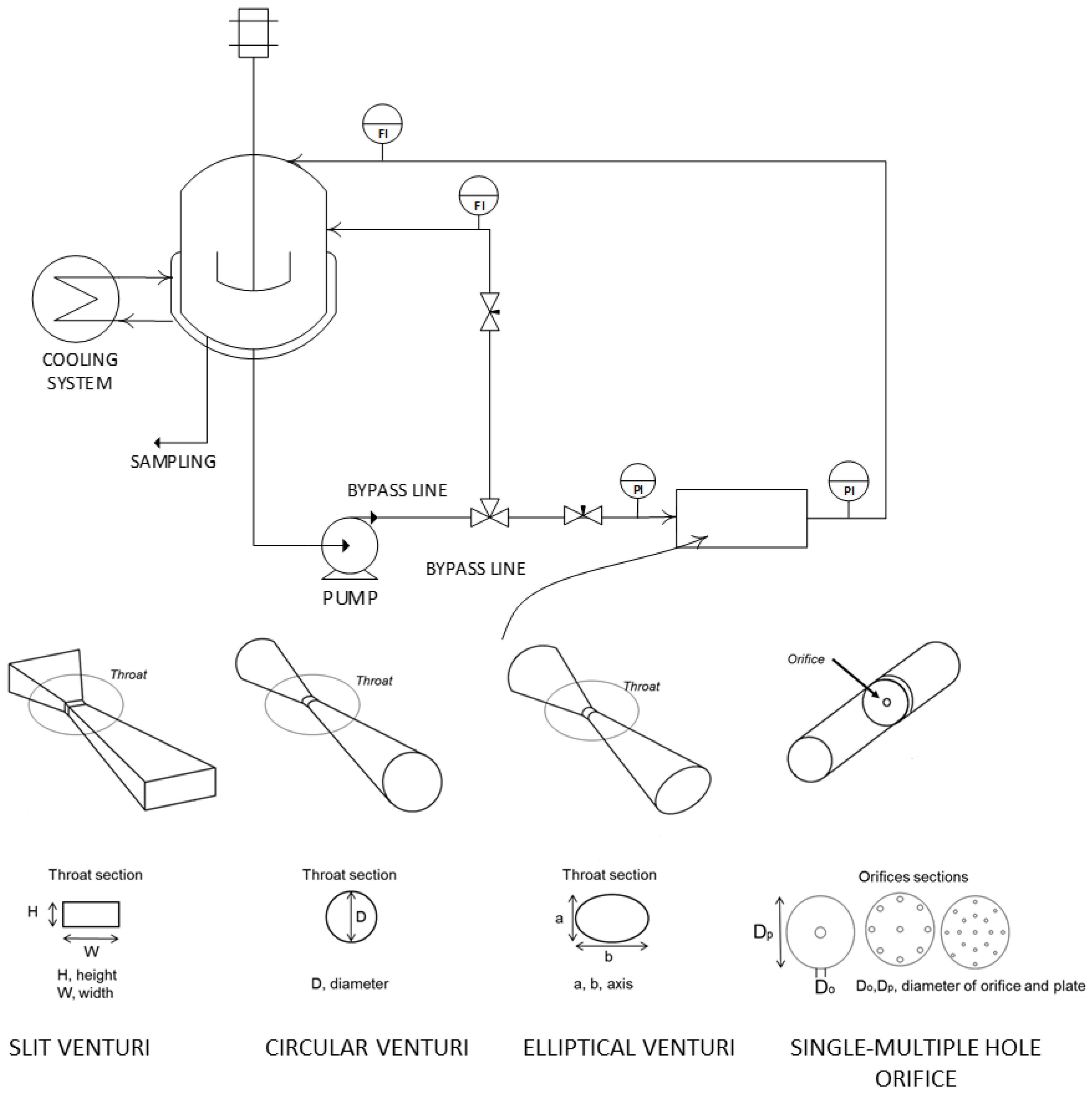
2.1. Summary of Reported Experimental Investigations

The typical lab scale experimental apparatus consists of the closed loop circuit sketched in Figure 1. This process scheme has been adopted (with limited modifications) in all the experimental works here analyzed [22,23,24,25,26,27,28,29,30,31,32,33,34,35,36,37,38,39,40,41,42,43]. It incorporates a stirred reactor (with cooling system), a recycling line, a centrifugal pump, pressure and flow meters, and two control valves. The temperature is controlled by a cooling water circuit, and the tank is stirred in order to ensure homogenous properties within the solution. The feed flowrate crosses the principal pipe and, passing through the cavitation device, reaches the tank. The liquid flow rate is regulated by using an additional by-pass line with a valve. Samples are withdrawn from the main tank and analyzed. The liquid sampling and the measurement of pollutant/oxidative species’ concentration occurs in the tank. Different analytical methods have been reported in the literature for the detection of pollutants including spectrophotometry, gas-liquid chromatography, and high-performance liquid chromatography (HPLC) [36,37,38,39,40,41,42]. Some works include the identification of byproducts generated by the cavitation treatment and depict possible degradation pathways [39]. Figure 1 also depicts the different “cavitational device” adopted in HC. Venturi is a converging duct followed by a diverging one, where the velocity is maximum at the throat corresponding to the minimum cross section [1,2,3,4]. Venturi devices present a divergent section with a smooth profile to avoid the sudden pressure recovery and to provide enough time for a cavity to remain in a low-pressure region and to reach maximum size before collapse. They can be of different shapes: slit, circular, and elliptical. The different sizes and shapes of the throat and divergent section can affect the number of cavitational events, the magnitude of the collapse pressure, and the residence time of the cavity in low-pressure region [11]. Two different types of materials are used in the fabrication of Venturi: acrylic used for photographic study and brass for the rest of the experiments with metal Venturi [21,22,23,24,25]. Orifice represents an alternative device for locally reducing pressure in a liquid flow motion. In single-hole orifice, the pressure recovers immediately, and the cavities collapse rapidly and with high intensity. Since the cavities are generated only at the edge of the throat, multiple-hole orifices are preferred to increase the cavitation event rate and the quantum of collapse pressure [11,12]. Throat size and shape also play an important role while designing the orifice-based HC; two important geometric parameters need to be considered in selecting the best configuration: α, defined as ratio of perimeter of the hole to the total flow area, and β, representing ratio of throat area to cross-sectional area of pipe [11,12].

The intensity of hydrodynamic cavitation and the related degradation yield depend on several parameters such as the inlet pressure, the geometry of a cavitating device as well as the physicochemical properties of the liquid (surface tension, density, and pH) which affect cavity generation rate and dynamics [10,11,12,24]. The dimensionless cavitation number (C_v), according to the following equation, is used to synthetize the fluid dynamics of the cavitation process [4,10,11,12,13,14,15,16,17,18,19,20,21,22,23,24,25]:

$${\mathrm{C}}_{\mathrm{v}}=\frac{{\mathrm{p}}_2-{\mathrm{p}}_{\mathrm{v}}}{0.5\times \mathsf{\rho } {{\mathrm{v}}_0}^2}$$

(1)

where p₂ is the fully recovered downstream pressure, p_v is the vapor pressure of the liquid, v₀ is the velocity at the throat of the cavitating constriction, and ρ is the density of liquid. The cavitation number corresponding to the inception of cavitation phenomenon is known as cavitation inception number, C_vi. Cavitation inception occurs at C_vi equal to 1, but relevant effects take place for C_v less than 1 [3]. By decreasing this number, the nucleation event rate increases as is visible in Figure 2.

Most of the experimental works refer to the C_v in describing the performances of the device. On the other hand, the group of University of Ljubljana pointed out the fact that the cavitation number cannot be used as a single parameter in describing the HC performances: also the geometry, the flow velocity, the liquid medium temperature, and quality strongly influence the cavitation dynamics [55]. More detailed fluid dynamic characterization of the HC devices can be found in the recent literature [56,57,58,59,60,61,62], and a recent comprehensive review has been published by Ferrari [63].

A literature investigation for the purpose of this work was carried out.

Table 1. Overview of studies considered for the aim of this work.

Cavitating Device	Pollutant	T (°C)	C0 (mg/L)	Pin (bar)	pH	Cv	K (min−1)	Reference
Venturi	Orange-G	32	13.6–67.9	3–7	2–9	0.11–0.21	5.25 × 10−4–3.10 × 10−2	Saharan et al., 2013 [22]
Venturi	Reactive Red 120	35	50	1–7	2–9	0.10–0.44	1.55 × 10−4–7.56 × 10−3	Saharan et al., 2011 [23]
Venturi	Acid red 88	30	20–60	3–7	2–10	0.11–0.21	5.80 × 10−4–2.35 × 10−2	Saharan et al., 2011 [24]
Venturi	Methyl orange	20	5	2–6.6	2–4	0.27–0.5	2.87 × 10−3–2.20 × 10−2	Innocenzi et al., 2018 [25]
Orifice	p-Nitrophenol	30	5000	0.4–2.9	6	0.26–0.53	2.58 × 10−3–7.96 × 10−3	Pradhan and Gogate, 2010 [26]
Circular Venturi			5000–10,000			0.46–0.56	3.29 × 10−3–8.48 × 10−3
Circular Venturi	Methylene blue dye	30	50	1–8	1–7.8	0.09–0.45	3.63 × 10−4–3.42 × 10−3	Kumar et al., 2017 [28]
Circular Venturi	Reactive Orange 4 dye	30	40	3–8	2	0.095–0.21	2.58 × 10−3–4.91 × 10−3	Gore et al., 2014 [30]
Slit Venturi	Dichlorvos	30	10–50	4–7	3–9	3–5	1.1 × 10−3–5.0 × 10−3	Thanekar et al., 2018 [31]
Venturi	Rhodamine B	30–40	10	2.9–5.8	2.5–11	0.07–0.20	1.26 × 10−3–8.77 × 10−3	Mishra and Gogate, 2010 [32]
Orifice		30			4.78	0.07–0.16	1.87 × 10−3–2.09 × 10−3
Slit Venturi	Carbamazepine	10	35	3–5	3–11.6		6.00 × 10−4–3.8 × 10−3	Thanekar et al., 2018 [33]
Orifice	Orange Acid II	20	20	3–7	2–8		2.24 × 10−3–5.67 × 10−3	Gogate and Boshale, 2013 [34]
Venturi	p-Nitrophenol	30	0.001	2–7	3.5–8	0.16–0.57	6.05 × 10−4–1.59 × 10−2	Capocelli et al., 2014 [35]
Orifice plate	2,4-dinitrophenol	30–40	20	3–6	3–11	-	7.7 × 10−4–1.11 × 10−3	Bagal et al., 2013 [36]
Orifice	Methyl parathion	30	20–100	1–8	2.2–8.2		1.40 × 10−3–5.42 × 10−3	Patil and Gogate, 2012 [37]
Orifice plate	Chlorpyrifos	31–39	0.11	3–8	3–10	0.35–3.47	8.02 × 10−3–4.14 × 10−2	Randhavane, 2019 [38]
Circular Venturi	Imidacloprid	32	25	3–20	2.7–7.5	0.051–0.215	2.42 × 10−4–2.89 × 10−3	Raut-Jadhav et al., 2014 [40]
Orifice	Ternary dyes	30	30	2–8	2–9	0.10–0.47	2.72 × 10−3–4.52 × 10−2	Kumar et al., 2018 [41]
Venturi	Tetramethyl ammonium hydroxide	20	2000	3.25–6	3–7	0.26–0.4	2.94 × 10−3–4.14 × 10−2	Innocenzi et al., 2018 [42]
Orifice	2-Amino-4-chlorophenol	35	20	2–4	3–8	0.27–0.76	1.7 × 10−3–1.9 × 10−3	Barik et al., 2016 [43]

synthetizes results of this survey, reporting the k_obs along with the main characteristic of the experimental works (type of device, pollutant, temperature, P_in, pH, C_v).

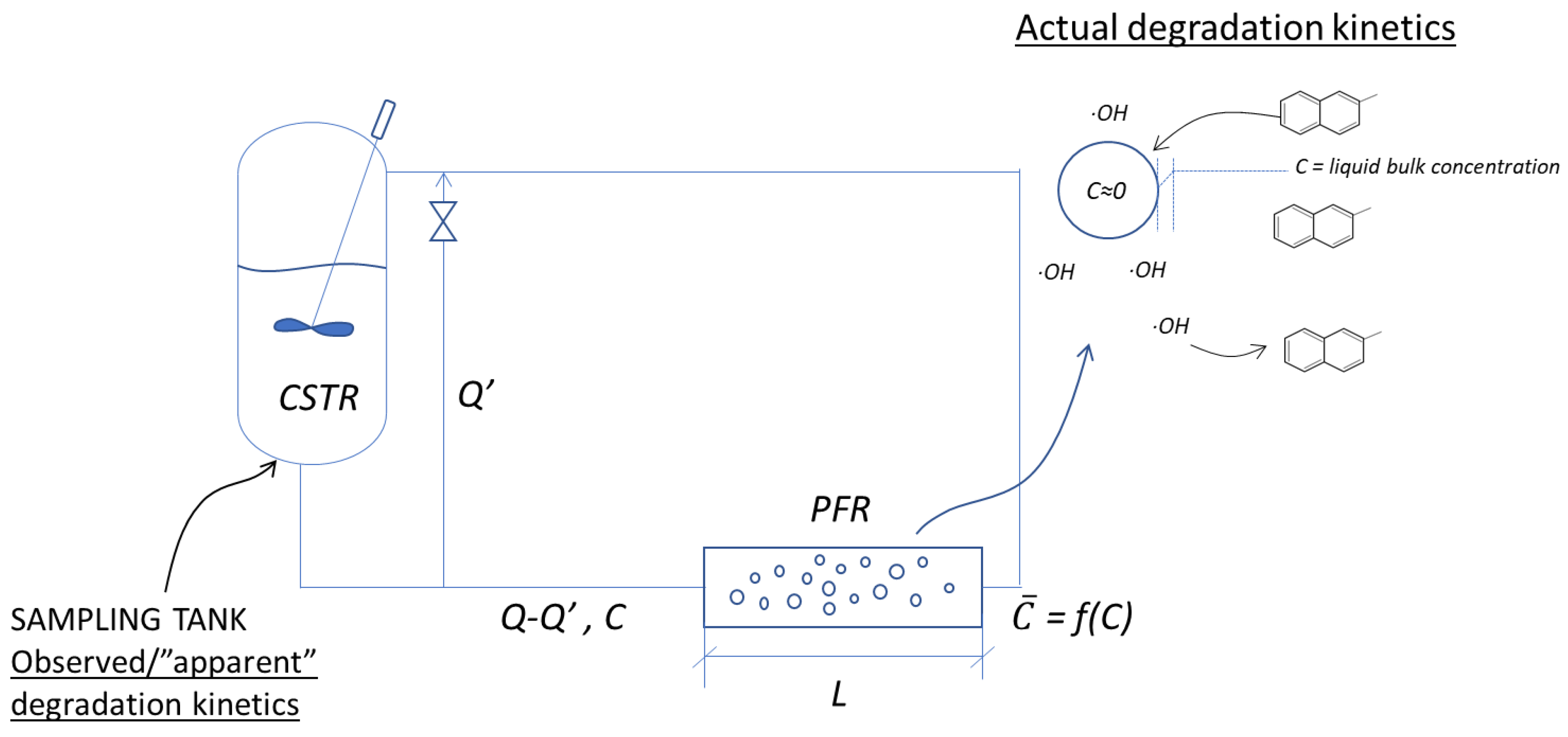
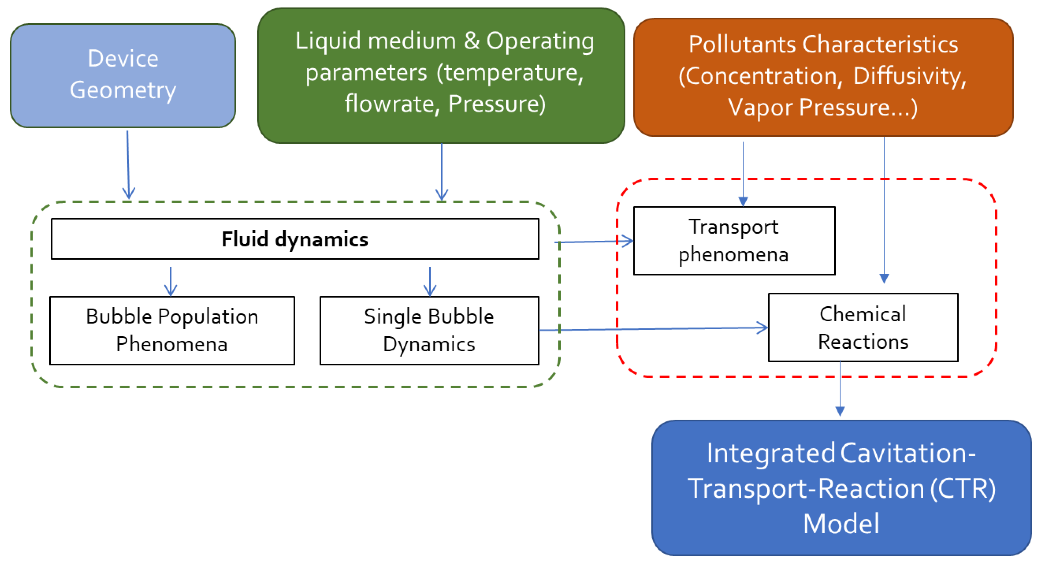
2.2. Mathematical Modeling

The modeling here proposed differs from the cited numerical studies [44,45,46,47,48,49,50,51,52] that rely on SBD approaches, but it is able to implement their results. In fact, our approach expands the observation area from the single bubble to whole HC apparatus. Figure 3 is a schematic of the conventional reactor with recirculation: the stirred thank where the degradation is “experimentally observed” can be seen as a CSTR (Continuous Stirred-Tank Reactor), and the zone interested by degradation is the PFR (Plug Flow Reactor) where the reactions occur through radical oxidation in the liquid bulk and diffusion followed by thermal degradation in the bubble. The sketch also includes the two circulation pipelines (principal and bypass line) with the related flowrate: Commonly, to control the flowrate, a portion of the total liquid volume is constantly recirculated, and the remaining part undergoes HC degradation inside the PFR reactor. Here, the pollutant concentration in the main line is reduced from C to $\overline{\mathrm{C}}$ for a single pass. Therefore, by including the simulation of the transport–reaction mechanisms occurring in the PFR and the mixing in the CSTR, the model aims to simulate the concentration at the sampling point to reproduce the experimental results.

The overall philosophy of the model, here called Cavitation–Transport–Reaction (CTR) model, is to integrate different results into a unifying approach; the interconnection between this novel approach and the other works available in the literature is depicted in Figure 4. The final aim of the CTR model is to reproduce the time variation of the pollutant concentration over time in the CSTR as well as to estimate the HC performances (e.g., cavitation yield) or to evaluate adjustable parameters (e.g., mass transfer coefficients) by fitting the experimental results.

By applying the mass balance (Equation (2)) to the sampling tank in Figure 3, it is possible to obtain the time dependence of the pollutant concentration C(t).

$$\frac{\mathrm{dC}}{\mathrm{dt}}=\frac{(\mathrm{Q}-{\mathrm{Q}}^{\prime })·(\mathrm{C}-\overline{\mathrm{C}})}{\mathrm{V}}$$

(2)

The relation between C and $\overline{\mathrm{C}}$ is discussed in the following. The concentration C(t), which has been experimentally observed in several works, is related to the reaction occurring in the cavitating zone. In this work, the “actual reactor” is modelled as a PFR: the flow, reaction, and dispersion of the pollutants are described by the second-order ordinary differential equation (Equation (3)). The two generations contributing to the pollutant degradation are: (i) reaction contribution governed by the reaction kinetic constant and (ii) diffusion term governed by the bulk-liquid diffusion towards the bubble boundary. The pollutant concentration inside the bubble is neglected because it undergoes a rapid thermal degradation occurring at the extreme conditions of collapse, and the bubble content consists of water vapor and its decomposition products.

$$\frac{{\mathrm{D}}_{\mathrm{L}}}{\mathrm{u}}\frac{{\mathrm{d}}^2\mathrm{C}}{{\mathrm{dz}}^2}-\frac{\mathrm{dC}}{\mathrm{dz}}-\frac{{\mathrm{K}}_{\mathrm{OH}}\times \mathrm{C}}{\mathrm{u}}-\frac{{\mathrm{K}}_{\mathrm{L}}\mathrm{a}\times \mathrm{C}}{\mathrm{u}}=0$$

(3)

$${\mathrm{K}}_{\mathrm{OH}}=\mathsf{\alpha }\times {{\mathrm{K}}^{\prime }}_{\mathrm{OH}}\times {\mathsf{\pi }}_{\mathrm{OH}}\times {\mathrm{n}}_{\mathrm{b}}$$

(4)

The global k_OH reaction constant is the product of the intrinsic reaction kinetic constant ${{\mathrm{K}}^{\prime }}_{\mathrm{OH}}$, the OH production rate per bubble ${\pi }_{\mathrm{OH}}$, the concentration (in number) of active bubbles n_b, and the availability factor α. This last parameter in particular represents the radical availability in the diffusion zone surrounding the bubble (as sketched in Figure 3) and varies depending on recombination and the scavenging effect of the liquid bulk (e.g., pH). Although the model parameters have not been experimentally estimated yet, they have a physical meaning and can be assumed (and verified with ad hoc experiments) or obtained by fitting experimental results.

The main assumption of this model is represented by the individuation of the controlling stage: the diffusion of pollutant at the interface between the liquid bulk and the bubble as depicted in Figure 3 (by assuming that in the bubble, the pollutant undergoes a thermal degradation). Hence, this first version of the model should be adapted to low-volatile compounds. The mass transfer model assumes that all resistance to interfacial mass transfer is localized in the liquid film at the interface (mass transfer controlled by the liquid film), while the liquid-side exchange coefficient k_La for a bubble reactor can be estimated from the literature, although ad hoc experiments for Venturi and orifice devices are needed [64]. Regarding the OH production rate per bubble ${\mathsf{\pi }}_{\mathrm{OH}}$, it is function of the collapse intensity, which in turn depends on the nuclei initial radius R₀ and fluid dynamics (inlet pressure P_in and geometry of the constriction). Several works estimated this parameter from the Single Bubble Dynamics (SBD) [44,54] as described in the Introduction. The reproduction of SBD results is left to other (more focused) numerical studies [21,35,46,47,48,49,50,51,52,53,54,55,56] and is out of the scope of this work, which aims to reproduce the overall phenomenology. Therefore, the ∙OH production rate is assumed from previous studies, according to the following correlation [49,50]:

$${\mathsf{\pi }}_{\mathrm{OH}}={{\mathrm{R}}_0}^{0.2428}\times {{\mathrm{P}}_{\mathrm{in}}}^{-4.6457}\times {({\mathrm{d}}_{\mathrm{o}}/{\mathrm{d}}_{\mathrm{p}})}^{-0.4732}$$

(5)

Few papers studied the dynamics of bubble population and reported the initial radii distribution (Equation (6)) as well as the nucleation event rate (Equation (7)), fundamental parameters in describing the HC phenomenology [5,61,62,63]. These equations have been assumed to obtain the preliminary results of the following sections but can be improved on the basis of optical measurements and ad hoc experiments in relation to the particular HC configuration.

$$\mathrm{N}({\mathrm{R}}_0)=\frac{\mathrm{b}}{{{\mathrm{R}}_0}^{\mathrm{m}}}$$

(6)

$$\mathrm{n}={\mathrm{n}}_0\frac{{\mathrm{p}}_{\mathrm{v}}-{\mathrm{p}}_{\min }}{{\mathrm{p}}_{\mathrm{v}}}$$

(7)

where b is the shape parameter of the bubble distribution function, n₀ is the number concentration of the pre-existent bubbles, p_v is the vapor pressure, and p_min the minimum pressure downstream the constriction.

Equation (3) can be written in dimensionless form by letting $\zeta =z/\mathrm{L}$ and $\phi =C/C_0$ and by introducing the Damköhler number, Da, for convection (Equation (9)), the Stanton number, St, for diffusion in the bubble (Equation (10)), and the Peclet number, Pe (Equation (11)).

$$\frac{1}{{\mathrm{Pe}}_{\mathrm{L}}}\frac{{\mathrm{d}}^2\mathsf{\phi }}{\mathrm{d}{\mathsf{\zeta }}^2}-\frac{\mathrm{d}\mathsf{\phi }}{\mathrm{d}\mathsf{\zeta }}-(\mathrm{Da}+\mathrm{St})\times \mathsf{\phi }=0$$

(8)

$$\mathrm{Da}=\frac{\mathrm{rate} \mathrm{of} \mathrm{consumption} \mathrm{by} \mathrm{reaction}}{\mathrm{rate} \mathrm{of} \mathrm{transport} \mathrm{by} \mathrm{convection}}=\frac{{\mathrm{K}}_{\mathrm{OH}}\mathrm{L}}{\mathrm{u}}$$

(9)

$$\mathrm{St}=\frac{\mathrm{residence} \mathrm{time} \mathrm{in} \mathrm{the} \mathrm{PFR}}{\mathrm{mass} \mathrm{transfer} \mathrm{time} \mathrm{scale}}=\frac{{\mathrm{K}}_{\mathrm{L}}\mathrm{a} \mathrm{L}}{\mathrm{u}}$$

(10)

$${\mathrm{Pe}}_{\mathrm{L}}=\frac{\mathrm{rate} \mathrm{of} \mathrm{transport} \mathrm{by} \mathrm{convection}}{\mathrm{rate} \mathrm{of} \mathrm{transport} \mathrm{by} \mathrm{dispersion}}=\frac{\mathrm{uL}}{{\mathrm{D}}_{\mathrm{L}}}$$

(11)

Assuming that there is no dispersion or radial variation in concentration either upstream or downstream of the reaction section (closed–closed vessel), the analytic solution of Equation (12) (with q-value explicated in Equation (13)) can be found from the Danckwerts’ boundary conditions.

$$\mathsf{\psi }=\frac{\overline{\mathrm{C}}}{\mathrm{C}}=1-\mathrm{X}=\frac{4\times \mathrm{q}\times \exp \left(\frac{\mathrm{Pe}}{2}\right)}{{(1-\mathrm{q})}^2\times \exp \left(\frac{\mathrm{Pe}\times \mathrm{q}}{2}\right)-{(1-\mathrm{q})}^2\times \exp \left(\frac{\mathrm{Pe}\times \mathrm{q}}{2}\right)}$$

(12)

$$\mathrm{q}=\sqrt{1+4\times (\mathrm{Da}+\mathrm{St})}$$

(13)

Once the analytical expression of the conversion through the PFR reactor has been obtained, it is possible to make explicit the "apparent" kinetic constant observed (k_obs) in the sampling volume V and replace Equation (1) with Equation (14). This approach allows to find the real link between experimental observations and process modeling.

$$\frac{\mathrm{dC}}{\mathrm{dt}}={\mathrm{k}}_{\mathrm{obs}}\times \mathrm{C}=\frac{(\mathrm{Q}-{\mathrm{Q}}^{\prime })\times (\mathrm{C}-\overline{\mathrm{C}})}{\mathrm{V}}=\frac{(\mathrm{Q}-{\mathrm{Q}}^{\prime })}{\mathrm{V}}\mathrm{X}\times \mathrm{C}$$

(14)

where k_obs is the degradation rate constant (min⁻¹).

3. Results and Discussion

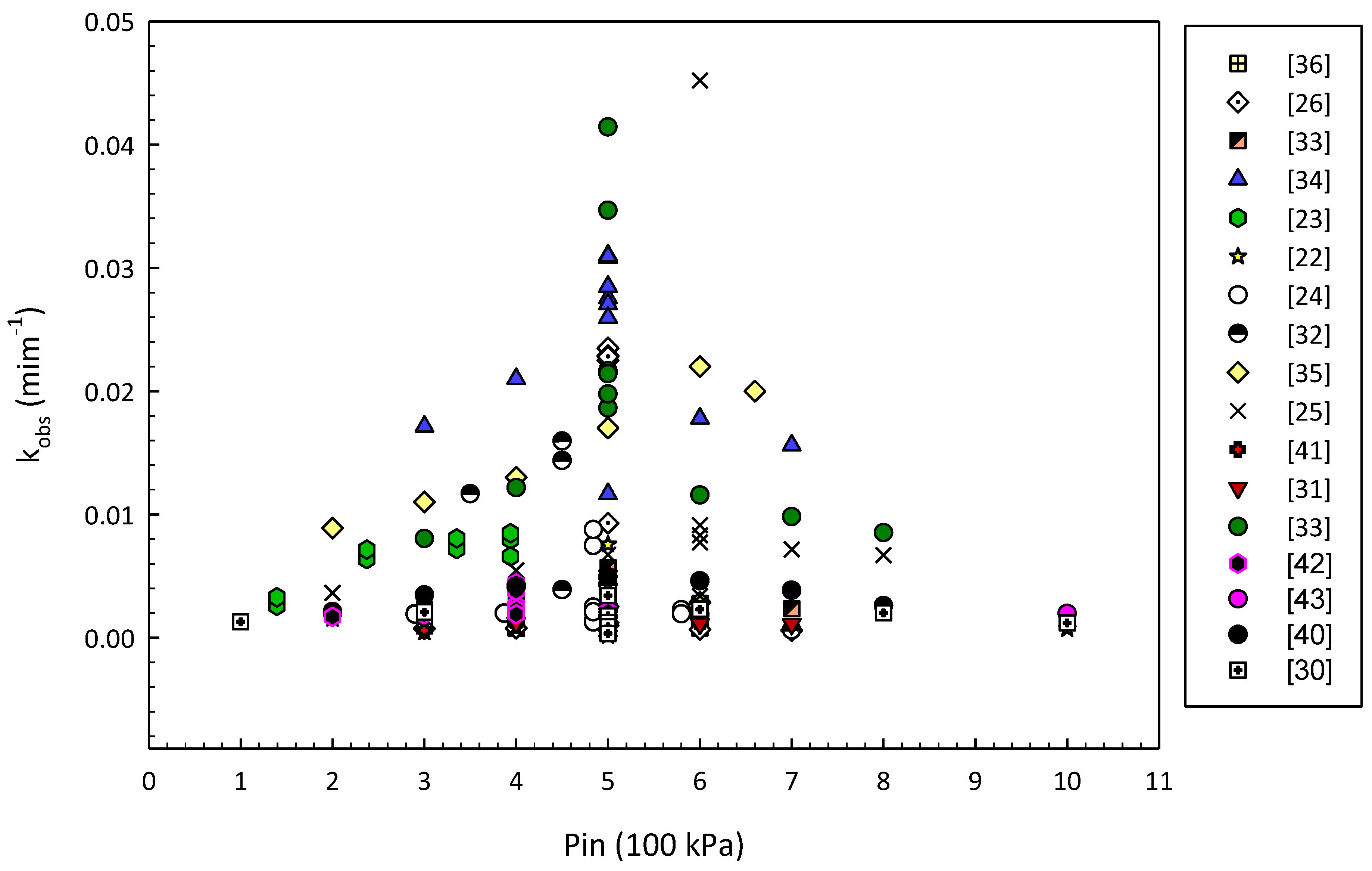
3.1. Experimental Observations

Equation (15) shows the observed first-order reaction, as reported by the experimental works object of this study.

$${\mathrm{C}}_{\mathrm{t}}={\mathrm{C}}_0\times \exp (-{\mathrm{k}}_{\mathrm{obs}}\mathrm{t})$$

(15)

where C₀ is the initial concentration and C_t the concentration at a time t. The effect of the most important operating parameter (P_in) on k_obs values (from the experimental work summarized in Table 1) is showed in Figure 5. Despite the diversity of molecules (very different molecular weight and logKow), the k_obs shows a maximum value at a “optimal” P_in around 5 bars.

Some discrepancies between different experiments derive, above all, from the different pH, which can have a negative effect on the kinetics, in particular, for the scavenging action of the radicals. Commonly, acidic pH of the solution favors the generation of OH radical also offering higher oxidation potential and lower rate of recombination of OH radicals. For example, Kumar Saharan conducted a set of constant pressure (5 bar) experiments, showing a clear negative effect of the pH [22,23,24]. To make the P_in effect more visible, the works with pH greater than 6 were eliminated and the dimensionless enhancing factor was calculated as k/k_min. Figure 6 shows the variation of the degradation constants and enhancing factors as a function of pressure, in particular a localized increase of enhancing factors with an order of magnitude of 10 for P_in values around 5 bars.

According to the literature, the most trivial reason for this is that, as the pressure increases, the flow rate in the main line increases so the liquid can go through the cavitating device several times and undergoes the AOP for a longer time. After reaching the maximum degradation rate at an optimal pressure, higher P_in values may produce the onset of super cavitation (i.e., indiscriminate growth of bubbles downstream of the constriction resulting in splashing and vaporization of the flow and in the formation of cavity cloud) having a negative effect on the HC process because of coalescence and reduced activity [20,29,34,35,36,37,38,39,40]. The modeling results in the next session will give more quantitative details.

From the correlation analysis of the aggregated data in relation to other parameters (such as those relating to the characteristics of pollutants) no clear correlations have been identified. From this preliminary study, it is not possible to find other clear relations between the summarized parameters and the k_obs, because of the predominant effect is certainly the input pressure. By including other variables and by preparing a larger set of data, a black-box approach could be implemented to develop more accurate predictive codes (“machine learning approach”). This topic is out of the scope of this work; some preliminary tentative examples can be found in the cited literature [65,66].

The effect of P_in appears independent from the characteristics of the molecule. This consideration allows us to use the CTR model to describe the fluid dynamic and mass transport effects on the k_obs, independently of the molecule under study. This reasoning allows to obtain general values and to identify the order of magnitude and the energy performance limits of the technology (regardless of the molecule).

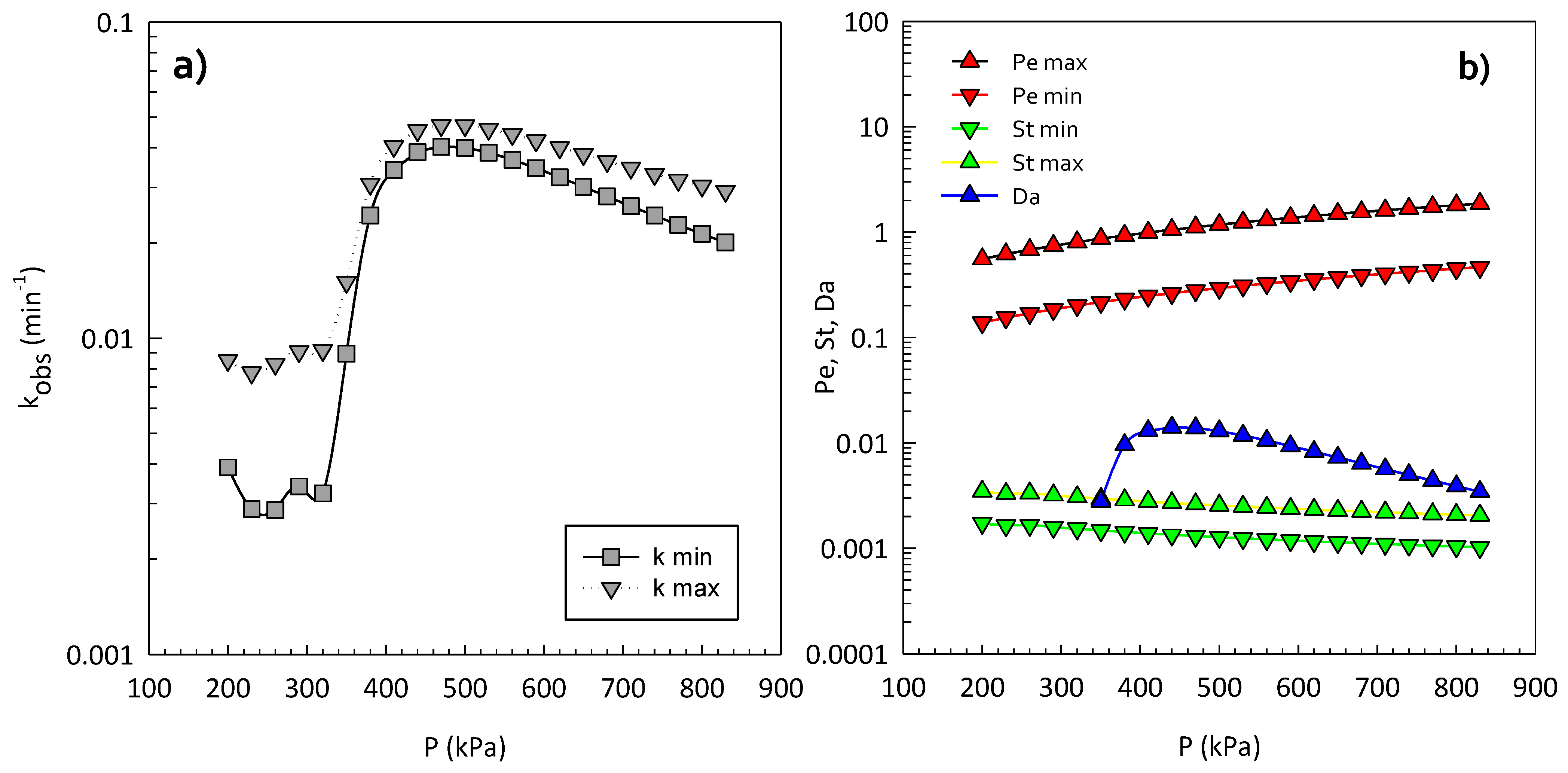
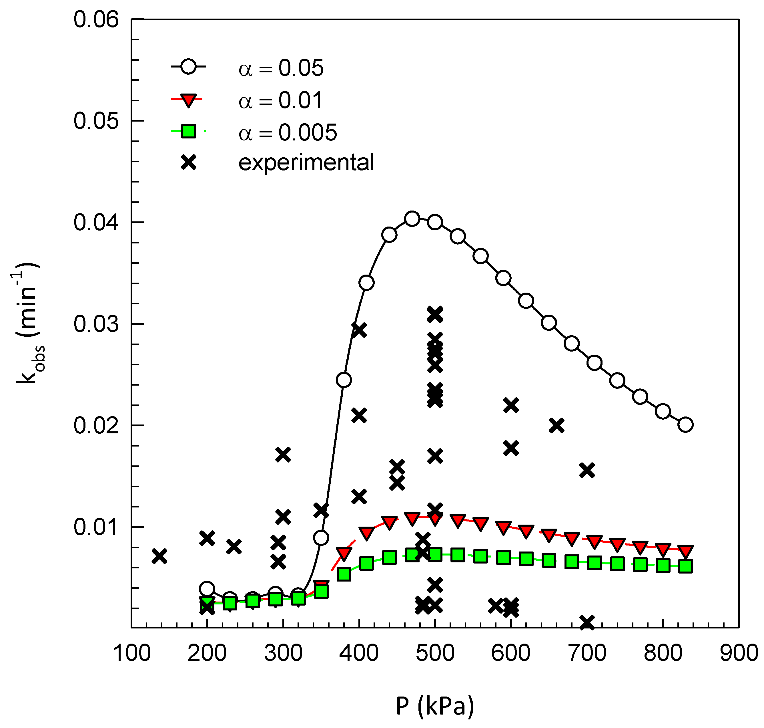
3.2. Simulation Results

The simulation results refer to the process scheme of Figure 3 with a Venturi device. The first results are based on the assumptions of some input parameters.

Table 2. Order of magnitude of the independent variables and main transport parameter for HC reactors (according to the experimental configuration of Ref. [39,51].

Variable	Description	Values
D (m)	Pipe diameter	0.012
D0 (m)	Orifice (constriction) diameter	0.002
Ld	Length of the divergent section	0.024
V (L)	Liquid volume	1.5
R0 (μm)	Initial bubble radius	50–150
πOH	Hydroxyl radical production at the collapse stage	Equation (5)
kLa (s−1)	Mass transfer coefficient	0.5–10 × 10−2
Dax (m2 s−1)	Axial Dispersion (eddy diffusivity)	0.02
kOH (M−1 s−1)	Hydroxyl radical—attack reaction rate	109

reports the value ranges assumed for the independent variables with some values varying in a fixed range for the purpose of a sensitivity analysis; ad hoc parameters can be experimentally estimated to improve the precision of the model on target molecules and particular geometries.

The first results are those relating to the fluid dynamics of the experimental circuit. As the inlet pressure increases, the flow rate circulating in the reactor and, therefore, the mechanical energy into the system increase. The geometry has a clear influence on the law that regulates the flow rate according to the head losses. Figure 7 shows the trends regarding the apparatus of our previous work [39].

Hence, the CTR model is implemented to predict the k_obs in the HC device with this fixed geometry and fluid-dynamics. The results are presented in relation to the inlet pressure P_in, which is the parameter that most influences the performances. The first sensitivity analysis is realized by varying the dimensionless numbers of Equation (8), in turn depending upon three parameters that need to be experimentally evaluated (D_ax, k_La, α). These values have been varied in a certain range to address their specific effect on the observed degradation rate. D_ax is assumed in the range 100–200 × 10⁻⁴ m²/s, and k_La has been calculated from the following equation with the parameter a in the range of 3 × 10⁻⁶–1 × 10⁻⁵ [64].

$${\mathrm{K}}_{\mathrm{L}}\mathrm{a}=\mathrm{a}\times {\left(\mathrm{D}\right)}^{-0.85}\times {\left(\mathrm{Re}\right)}^{0.52}$$

(16)

Figure 8a reports the k_obs calculated at different P_in for the maximum and minimum values assumed for D_ax (influencing the Pe number) and the k_La (influencing the St number). Da number has been calculated by fixing the availability parameter α at 0.05. For the parameter variation in the chosen range, minimum and maximum values have been reported. From Figure 8a, it is possible to observe a peak of k_obs corresponding to the optimal inlet pressure of 5 bar. On the other hand, Figure 8b reports the range of the calculated dimensionless numbers. While Pe slightly increases and St slightly decreases as the P_in increases, the trend of Da number is influenced by the contrasting effect of two contributions: (i) increasing nucleation event rate at higher pressure and (ii) the simultaneous reduction of collapse intensity and (consequently) of radical specific production at high pressures (Equation (5)). The dichotomy between convection and reaction precisely produces a maximum in the curve relative to the kinetic constants in correspondence to P_in values around 5 bar, as experimentally observed from the aggregate values of Figure 5 and Figure 6. Although these values depend on the parameter assumptions, they reflect the trends observed in the cited works (see Table 1 and Figure 5 and Figure 6) that cover a wide variation of experimental conditions (from geometry to the characteristics of the chemical species and/or presence of scavengers in solution).

For model validation with experimental data, the results of experiments performed with similar pollutants (Venturi device at pH lower than 6 reported in [25,26,35,42]) were presented in Figure 9, along with results of three model simulations realized at three values of the scavenging parameter α (with D_ax = 150 × 10⁻⁴ m² s⁻¹). According to the state of approximation and current generality of the model, this trend is valid for any pollutant as long as the k_OH is 10⁻⁹ (M⁻¹ s⁻¹). It should be noted that the pollutants (listed in Table 1) are among the most common organic micropollutants (mainly aromatics) studied for AOP and include the categories of drugs, pesticides, and dyes. Precisely for this reason, the results reported in this work can be taken, albeit as preliminary, as extendable to the HC process and not to the particular pollutant. By observing the results of Figure 9, it is possible to state that the model reproduces well the large number of experimental data realized by different authors with “similar but heterogeneous” experimental conditions. The fitting of the transport parameters was not carried out because the simulations embrace a variety of experiments with different geometry (therefore fluid dynamic behavior) and different characteristics of the aqueous matrix or pollutants. In fact, the model is used as a predictor by setting the parameters as aforementioned for the sensitivity analysis. The mean squared error (MSE) between the simulations and the experimental values of Figure 9 are reported in Figure 10. As for this global simulation and on the basis of the preliminary assumptions, the optimal value of the parameter α (that minimizes the MSE) is around 0.02. Although more ad hoc experiments for the estimation of the optimal values of the model parameters are needed, it represents a first step towards the introduction of CTR models in the description of the HC phenomenology.

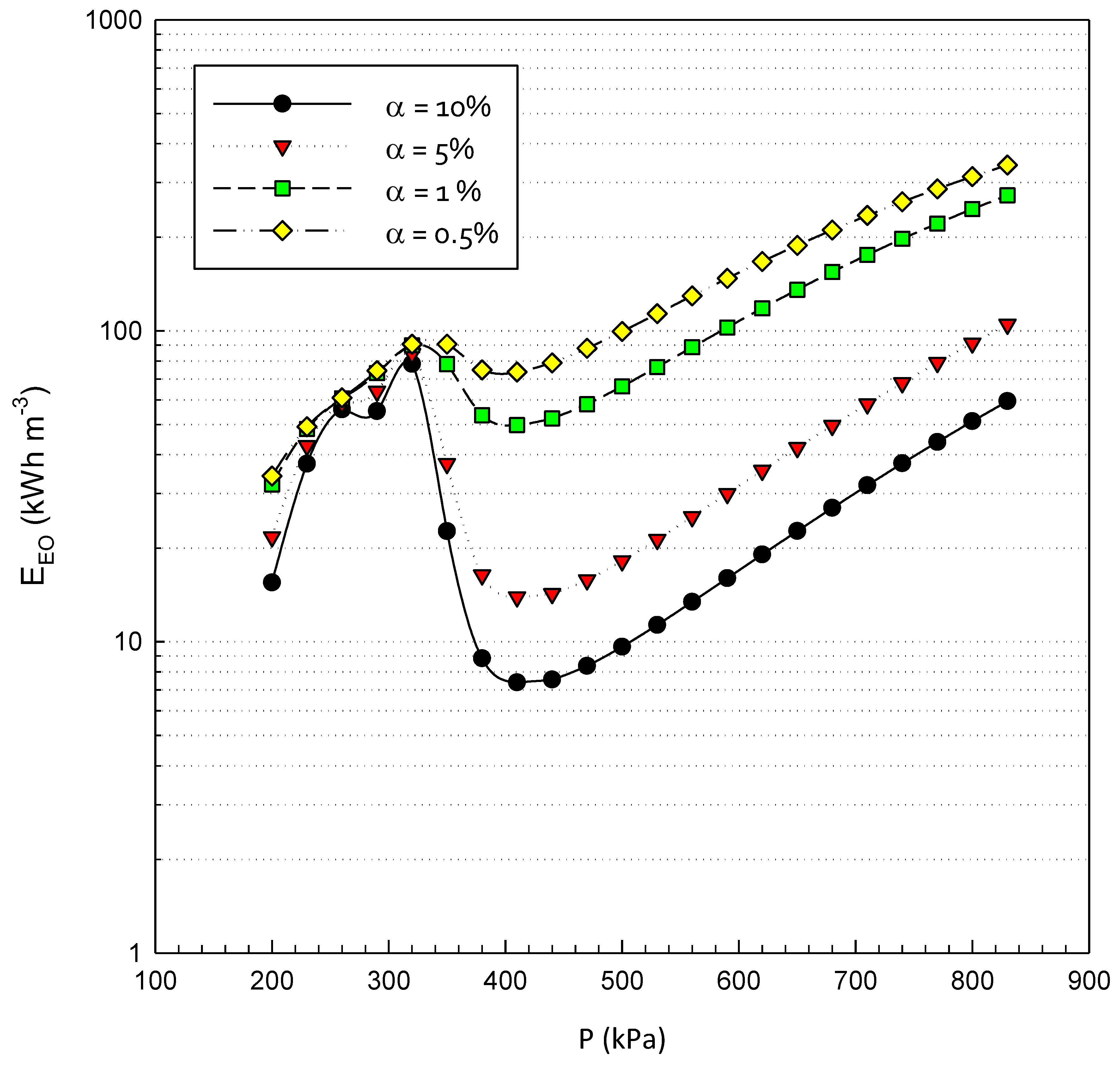
3.3. Energy Efficiency

From these results, it is also possible to look at orders of magnitude of the energy efficiency that directly links the fluid dynamics to the degradation performance.

In HC, the mechanical energy provided by the centrifugal pump downstream the constriction is converted into (1) residual kinetic and pressure energy, (2) turbulent dissipation and thermal effects, and (3) bubble compression and thermal decomposition of vapor and generation of radical species. Energy consumption is calculated from Equation (17) as electrical efficiency per order E_EO, specialized by Bolton et al. for first-order kinetics [67]. The simulation is repeated for different values of the scavenging parameter α and the results are plotted versus the variable P_in in Figure 11.

$${\mathrm{E}}_{\mathrm{Eo}}=\frac{{\mathrm{N}}_{\mathrm{p}}\mathsf{\tau }\times 1000}{\mathrm{V}\times \log \left(\frac{{\mathrm{C}}_0}{{\mathrm{C}}_{\mathrm{t}}}\right){\mathsf{\eta }}_{\mathrm{p}}}=\frac{38.4 {\mathrm{N}}_{\mathrm{p}}}{\mathrm{V}\times {\mathrm{K}}_{\mathrm{obs}}}$$

(17)

where, according to the formulation of Bolton et al. [67], Np is the pump power in kW, V is the total volume of the treated water in L, $\mathsf{\tau }$ is the time to reach the concentration C_t, and η_p is the pump efficiency.

It can be seen that as the P_in increases, the minimum energy consumption is obtained around 400 kPa, in proximity of the highest values obtained for k_obs; further P_in increases lead to higher energy consumption. This is because the power requirement at higher pressure and flow rate (see Figure 7) does not result in a higher enough degradation rate. The minimum value can be individuated in the optimal P_in around 400–500 kPa (therefore individuated as optimal pressure). Over this range of 400–500 kPa, the energy input is not transformed into the chemical effect (advanced oxidation), and there is a considerable power dissipation (thermo-mechanical effects of cavitation).

Although the E_EO for industrial processes can differ by one or two orders of magnitude and depends on the process parameters as well as the scale of the apparatus, our results are comparable to the ones reported in the literature and related to the refence AOP. The minimum value of 7 kWh/m³ observed at 400 kPa is below the E_EO of ultrasonic cavitation, as commonly demonstrated in the scientific literature [8,10,12,67,68,69,70,71] and is in the range of Ozonation, O₃/H₂O₂, UV/persulfate, O₃/UV UV/H₂O₂ [67,68,69,70,71,72,73]. Moreover, these values have been obtained for pure hydrodynamic cavitation and can be consistently decreased by the application of hybrid techniques including cavitation and H₂O₂ or O₃.

4. Conclusions

Hydrodynamic cavitation (HC) has been extensively studied for the Advanced Oxidation of organic compounds from both experimental and theoretical points of view. This process is simple and economical because of its capability for generating hydroxyl radicals under ambient conditions, its ease of scale-up, and its lower material costs [10,11,14]. It can be included in retrofit solutions because it only requires the insertion of a properly designed restriction of the outflow section in a pipeline.

Several works individuated similar optimal operating conditions, especially with regard to the inlet pressure on the cavitation reactor. Moreover, most of the modeling works obtained important results on the dynamics of bubbles and cavitation reactions but did not consider the overall phenomenology of the HC systems. At the moment no one reported a clear link between the models and the experimental results.

In this work, a first attempt in this sense has been made. First, the paper presents a survey of several experimental works. After that, a novel model based on transport phenomena within the reactor is proposed. It includes and interconnects several literature results in a novel architecture to obtain quantitative and qualitative information on the pollutants’ degradation. Although it is still to be improved, the first comparisons with literature are encouraging since the proposed model is able to predict k_obs in the HC device with fixed geometry and fluid-dynamics. For D_ax and k_La assumed at maximum and minimum values, simulation results report that k_obs, as function of P_in, reached the highest pressure value close to 5 bars, confirming experimental results from the literature. In addition, focusing on results of experiments performed with Venturi devices, at pH lower than 6, the comparison of three model simulations realized at three values of the scavenging parameter α (with D_ax = 150 × 10⁻⁴ m² s⁻¹) and experimental results allows to state that this model will simulate the large number of experimental data obtained by different authors. Within this global simulation, the best value of the scavenging parameter α was 2%. A careful estimation of this and the main transport parameters will be carried out with ad hoc experimental campaigns.

With the same model assumption, the electrical efficiency per order has been estimated and compared with literature results finding the optimal value around 7 kWh/m³ close to 400 kPa of inlet pressure. Globally, these values justify the implementation of HC as an AOP. On the other hand, the energy consumption is not “universally low” if compared to the energy requirement of water technologies and for “real-effluent” applications, the process yield can decrease in the presence of several pollutants and scavengers at higher concentrations [67,68,69,70]. It is important to state that better results can be obtained in hybrid applications (concomitantly with chemical AOP and cavitation) [67,69,70,71] since the main advantage of HC is to offer an environment favorable to oxidation and thermal degradation and to improve the performances of the main chemical AOPs.

Although the model still presents some elements to improve, it represents the first approach able to directly simulate a large number of experimental data obtained in different conditions, with different apparatus and different molecules. The elements that could characterize future developments are the following:

• To implement this model, by fitting ad hoc experimental results, to estimate the model parameters that cannot be directly know from the literature.
• To improve the model for volatile compounds undergoing thermal degradation into the bubble environment.
• To evaluate the scavenging effect by means of ad hoc experiments and model fitting on the variable α.
• To test the model and to optimize the HC process for different geometries.
• To address the energy efficiency and the theoretical limit of HC from a thermodynamic point of view.

References

1. Maršálek, B.; Maršálková, E.; Odehnalová, K.; Pochylý, F.; Rudolf, P.; Stahel, P.; Rahel, J.; Čech, J.; Fialová, S.; Zezulka, Š. Removal of Microcystis aeruginosa through the Combined Effect of Plasma Discharge and Hydrodynamic Cavitation. Water 2020, 12, 8. [Google Scholar] [CrossRef] [Green Version]
2. Gogate, P.R.; Kabadi, A.M. A Review of Applications of Cavitation in Biochemical Engineering/Biotechnology. Biochem. Eng. J. 2009, 44, 60–72. [Google Scholar] [CrossRef]
3. Gogate, P.R. Cavitation: An Auxiliary Technique in Wastewater Treatment Schemes. Adv. Environ. Res. 2002, 6, 335–358. [Google Scholar] [CrossRef]
4. Franc, J.-P.; Michel, J.-M. Fundamentals of Cavitation; Springer Science & Business Media: Berlin, Germany, 2005. [Google Scholar] [CrossRef]
5. Cuerda-Correa, E.M.; Alexandre-Franco, M.F.; Fernandez-Gonzalez, C. Advanced Oxidation Processes for the Removal of Antibiotics from Water. An Overview. Water 2020, 12, 102. [Google Scholar] [CrossRef] [Green Version]
6. Gogate, P.R. Cavitational Reactors for Process Intensification of Chemical Processing Applications: A Critical Review. Chem. Eng. Process. 2008, 47, 515–527. [Google Scholar] [CrossRef]
7. Young, F.R. Cavitation; McGraw-Hill Book Co Ltd.: London, UK, 1989. [Google Scholar]
8. Gogate, P.R.; Patil, P.N. Sonochemical Reactors, Topics in Current Chemistry; Springer International Publishing: Cham, Switzerland, 2016; Volume 374, pp. 1–27. [Google Scholar] [CrossRef]
9. Mason, T.J.; Lorimer, J.P. Applied Sonochemistry: The Uses of Power Ultrasound in Chemistry and Processing; Wiley-VCH Verlag GmbH: Weinheim, Germany, 2002. [Google Scholar] [CrossRef]
10. Saharan, V.K.; Pinjari, D.V.; Gogate, P.R.; Pandit, A.B. Industrial Wastewater Treatment, Recycling and Reuse; Advanced Oxidation Technologies for Wastewater Treatment: An Overview; Butterworth-Heinemann: Oxford, UK, 2014. [Google Scholar] [CrossRef]
11. Carpenter, J.; Badve, M.; Rajoriya, S.; George, S.; Saharan, V.K.; Pandit, A.B. Hydrodynamic Cavitation: An Emerging Technology for the Intensification of Various Chemical and Physical Processes in a Chemical Process Industry. Rev. Chem. Eng. 2016, 33, 433–468. [Google Scholar] [CrossRef]
12. Gogate, P.R.; Pandit, A.B. Engineering Design Method for Cavitational Reactors: II. Hydrodynamic Cavitatiom. AIChE J. 2000, 46, 1641–1649. [Google Scholar] [CrossRef]
13. Gogate, P.R.; Tatake, P.A.; Kanthale, P.M.; Pandit, A.B. Mapping of Sonochemical Reactors: Review, Analysis, and Experimental Verification. AIChE J. 2002, 48, 1542–1560. [Google Scholar] [CrossRef]
14. Bagal, M.V.; Gogate, P.R. Wastewater Treatment Using Hybrid Treatment Schemes Based on Cavitation and Fenton Chemistry: A Review. Ultrason. Sonochem. 2014, 21, 1–14. [Google Scholar] [CrossRef]
15. González-García, J.; Sáez, V.; Tudela, I.; Díez-Garcia, M.I.; Esclapez, M.D.; Louisnard, O. Sonochemical Treatment of Water Polluted by Chlorinated Organocompounds. A Review. Water 2010, 2, 28–74. [Google Scholar] [CrossRef]
16. Wang, C.; Ying, Z.; Ma, M.; Huo, M.; Yang, W. Degradation of Micropollutants by UV–Chlorine Treatment in Reclaimed Water: pH Effects, Formation of Disinfectant Byproducts, and Toxicity Assay. Water 2019, 11, 2639. [Google Scholar] [CrossRef] [Green Version]
17. Capocelli, M.; Joyce, E.; Lancia, A.; Mason, T.J.; Musmarra, D.; Prisciandaro, M. Sonochemical Degradation of Estradiols: Incidence of Ultrasonic Frequency. Chem. Eng. J. 2012, 210, 9–17. [Google Scholar] [CrossRef]
18. Thanekar, P.; Gogate, P.R. Combined Hydrodynamic Cavitation Based Processes as an Efficient Treatment Option for Real Industrial Effluent. Ultrason. Sonochem. 2019, 53, 202–213. [Google Scholar] [CrossRef] [PubMed]
19. Chakinala, A.G.; Gogate, P.R.; Chand, R.; Bremner, D.H.; Molina, R.; Burgess, A.E. Intensification of Oxidation Capacity Using Chloroalkanes as Additives in Hydrodynamic and Acoustic Cavitation Reactors. Ultrason. Sonochem. 2008, 15, 64–170. [Google Scholar] [CrossRef] [PubMed]
20. Tao, Y.; Cai, J.; Huai, X.; Liu, B.; Guo, Z. Application of Hydrodynamic Cavitation to Wastewater Treatment. Chem. Eng. Technol. 2016, 39, 1363–1376. [Google Scholar] [CrossRef]
21. Capocelli, M.; Prisciandaro, M.; Musmarra, D.; Lancia, A. Understanding the Physics of Advanced Oxidation in a Venturi Reactor. Chem. Eng. Trans. 2013, 32, 691–696. [Google Scholar] [CrossRef]
22. Saharan, V.K.; Rizwani, M.A.; Malani, A.A.; Pandit, A.B. Effect of Geometry of Hydrodynamically Cavitating Device on Degradation of Orange-G. Ultrason. Sonochem. 2013, 20, 345–353. [Google Scholar] [CrossRef]
23. Saharan, V.K.; Badve, M.P.; Pandit, A.B. Degradation of Reactive Red 120 Dye Using Hydrodynamic Cavitation. Chem. Eng. J. 2011, 178, 100–107. [Google Scholar] [CrossRef]
24. Saharan, V.K.; Pandit, A.B.; Satish Kumar, P.S.; Anandan, S. Hydrodynamic Cavitation as an Advanced Oxidation Technique for the Degradation of Acid Red 88 Dye. Ind. Eng. Chem. Res. 2012, 51, 1981–1989. [Google Scholar] [CrossRef]
25. Innocenzi, V.; Prisciandaro, M.; Tortora, F.; Vegliò, F. Optimization of Hydrodynamic Cavitation Process of Azo Dye Reduction in the Presence of Metal Ions. J. Environ. Chem. Eng. 2018, 6, 6787–6796. [Google Scholar] [CrossRef]
26. Pradhan, A.A.; Gogate, P.R. Removal of P-Nitrophenol Using Hydrodynamic Cavitation and Fenton Chemistry at Pilot Scale Operation. Chem. Eng. J. 2010, 156, 77–82. [Google Scholar] [CrossRef]
27. Thanekar, P.; Murugesan, P.; Gogate, P.R. Improvement in Biological Oxidation Process for the Removal of Dichlorvos from Aqueous Solutions Using Pretreatment Based on Hydrodynamic Cavitation. J. Water Process Eng. 2018, 23, 20–26. [Google Scholar] [CrossRef]
28. Kumar, M.S.; Sonawane, S.H.; Pandit, A.B. Degradation of Methylene Blue Dye in Aqueous Solution Using Hydrodynamic Cavitation Based Hybrid Advanced Oxidation Processes. Chem. Eng. Process. 2017, 122, 288–295. [Google Scholar] [CrossRef]
29. Wang, X.; Zhang, Y. Degradation of Alachlor in Aqueous Solution by Using Hydrodynamic Cavitation. J. Hazard. Mater. 2009, 161, 202–207. [Google Scholar] [CrossRef]
30. Gore, M.M.; Saharan, V.K.; Pinjari, D.V.; Chavan, P.V.; Pandit, A.B. Degradation of Reactive Orange 4 Dye Using Hydrodynamic Cavitation Based Hybrid Techniques. Ultrason. Sonochem. 2014, 21, 1075–1082. [Google Scholar] [CrossRef]
31. Thanekar, P.; Panda, M.; Gogate, P.R. Degradation of Carbamazepine Using Hydrodynamic Cavitation Combined with Advanced Oxidation Processes. Ultrason. Sonochem. 2018, 40, 567–576. [Google Scholar] [CrossRef]
32. Mishra, K.P.; Gogate, P.R. Intensification of Degradation of Rhodamine B Using Hydrodynamic Cavitation in the Presence of Additives. Sep. Purif. Technol. 2010, 75, 385–391. [Google Scholar] [CrossRef]
33. Thanekar, P.; Gogate, P.R. Application of Hydrodynamic Cavitation Reactors for Treatment of Wastewater Containing Organic Pollutants: Intensification Using Hybrid Approaches. Fluids 2018, 3, 98. [Google Scholar] [CrossRef] [Green Version]
34. Gogate, P.R.; Bhosale, G.S. Comparison of Effectiveness of Acoustic and Hydrodynamic Cavitation in Combined Treatment Schemes for Degradation of Dye Wastewaters. Chem. Eng. Process. 2013, 71, 59–69. [Google Scholar] [CrossRef]
35. Capocelli, M.; Prisciandaro, M.; Lancia, A.; Musmarra, D. Hydrodynamic Cavitation of P-Nitrophenol: A Theoretical and Experimental Insight. Chem. Eng. J. 2014, 254, 1–8. [Google Scholar] [CrossRef]
36. Bagal, M.V.; Gogate, P.R. Degradation of 2,4-Dinitrophenol Using a Combination of Hydrodynamic Cavitation, Chemical and Advanced Oxidation Processes. Ultrason. Sonochem. 2013, 20, 1226–1235. [Google Scholar] [CrossRef] [PubMed]
37. Patil, P.N.; Gogate, P.R. Degradation of Methyl Parathion Using Hydrodynamic Cavitation: Effect of Operating Parameters and Intensification Using Additives. Sep. Purif. Technol. 2012, 95, 172–179. [Google Scholar] [CrossRef]
38. Randhavane, S.B. Comparing Geometric Parameters of a Hydrodynamic Cavitation Process Treating Pesticide Effluent. Environ. Eng. Res. 2018, 24, 318–323. [Google Scholar] [CrossRef] [Green Version]
39. Musmarra, D.; Prisciandaro, M.; Capocelli, M.; Karatza, D.; Iovino, P.; Canzano, S.; Lancia, A. Degradation of Ibuprofen by Hydrodynamic Cavitation: Reaction Pathways and Effect of Operational Parameters. Ultrason. Sonochem. 2016, 29, 76–83. [Google Scholar] [CrossRef]
40. Raut-Jadhav, S.; Saharan, V.K.; Pinjari, D.; Sonawane, S.; Saini, D.; Pandit, A. Synergetic Effect of Combination of AOP’s (Hydrodynamic Cavitation and H2O2) on the Degradation of Neonicotinoid Class of Insecticide. J. Hazard. Mater. 2013, 261, 139–147. [Google Scholar] [CrossRef]
41. Kumar, M.S.; Sonawane, S.H.; Bhanvase, B.A.; Bethi, B. Treatment of Ternary Dye Wastewater by Hydrodynamic Cavitation Combined with Other Advanced Oxidation Processes (AOP’s). J. Water Process Eng. 2018, 23, 250–256. [Google Scholar] [CrossRef]
42. Innocenzi, V.; Prisciandaro, M.; Vegliò, F. Effect of the Hydrodynamic Cavitation for the Treatment of Industrial Wastewater. Chem. Eng. Trans. 2018, 67, 529–534. [Google Scholar] [CrossRef]
43. Barik, A.J.; Gogate, P.R. Degradation of 4-Chloro 2-Aminophenol Using a Novel Combined Process Based on Hydrodynamic Cavitation, UV Photolysis and Ozone. Ultrason. Sonochem. 2016, 30, 70–78. [Google Scholar] [CrossRef]
44. Moholkar, V.S.; Pandit, A.B. Bubble Behavior in Hydrodynamic Cavitation: Effect of Turbulence. AIChE J. 1997, 43, 1641–1648. [Google Scholar] [CrossRef]
45. Moholkar, V.S.; Senthil Kumar, P.; Pandit, A.B. Hydrodynamic Cavitation for Sonochemical Effects. Ultrason. Sonochem. 1999, 6, 53–65. [Google Scholar] [CrossRef]
46. Storey, B.D.; Szeri, J. Water vapour, sonoluminescence and sonochemistry. Proc. R. Soc. A Math. Phys. Eng. Sci. 2000, 456, 1685–1709. [Google Scholar] [CrossRef]
47. Toegel, R.; Gompf, B.; Pecha, R.; Lohse, D. Does Water Vapor Prevent Upscaling Sonoluminescence? Phys. Rev. Lett. 2000, 85, 3165–3168. [Google Scholar] [CrossRef] [PubMed] [Green Version]
48. Kumar, P.; Khanna, S.; Moholkar, V. Flow regime maps and optimization thereby of hydrodynamic cavitation reactors. AIChE J. 2012, 58, 3858–3866. [Google Scholar] [CrossRef]
49. Sharma, A.; Gogate, P.; Mahulkar, A.; Pandit, A. Modeling of hydrodynamic cavitation reactors based on orifice plates considering hydrodynamics and chemical reactions occurring in bubble. Chem. Eng. J. 2008, 143, 201–209. [Google Scholar] [CrossRef]
50. Krishnan, J.S.; Dwivedi, P.; Moholkar, V.S. Numerical Investigation into the Chemistry Induced by Hydrodynamic Cavitation. Ind. Eng. Chem. Res. 2006, 45, 1493–1504. [Google Scholar] [CrossRef]
51. Capocelli, M.; Musmarra, D.; Prisciandaro, M.; Lancia, A. Chemical Effect of Hydrodynamic Cavitation: Simulation and Experimental Comparison. AIChE J. 2014, 60, 2566–2572. [Google Scholar] [CrossRef]
52. Mishra, S.K.; Deymier, P.; Muralidharan, K.; Frantziskonis, G.; Pannala, S.; Simunovic, S. Modeling the coupling of reaction kinetics and hydrodynamics in a collapsing cavity. Ultrason. Sonochem. 2010, 17, 258–265. [Google Scholar] [CrossRef]
53. Ozonek, J. Application of Hydrodynamic Cavitation in Environmental Engineering; CRC Press: London, UK, 2012. [Google Scholar]
54. Dular, M.; Coutier-Delgosha, O. Thermodynamic effects during growth and collapse of a single cavitation bubble. J. Fluid Mech. 2013, 736, 4466. [Google Scholar] [CrossRef] [Green Version]
55. Šarc, A.; Stepišnik-Perdih, T.; Petkovšek, M.; Dular, M. The issue of cavitation number value in studies of water treatment by hydrodynamic cavitation. Ultrason. Sonochem. 2016, 34, 51–59. [Google Scholar] [CrossRef]
56. Ladino, J.A.; Herrera, J.; Malagon, D.; Prisciandaro, M.; Piemonte, V.; Capocelli, M. Biodiesel production via hydrodynamic cavitation: Numerical study of new geometrical arrangements. Chem. Eng. Trans. 2016, 50, 319–324. [Google Scholar] [CrossRef]
57. Delale, C.F.; Okita, K.; Matsumoto, Y. Steady-State Cavitating Nozzle Flows With Nucleation. J. Fluids Eng. 2005, 127, 770–777. [Google Scholar] [CrossRef]
58. Yan, Y.; Thorpe, R.B. Flow regime transitions due to cavitation in the flow through an orifice. Int. J. Multiph. Flow 1990, 16, 1023–1045. [Google Scholar] [CrossRef]
59. Bashir, T.A.; Soni, A.G.; Mahulkar, A.V.; Pandit, A.B. The CFD driven optimization of a modified venturi for cavitational activity. Can. J. Chem. Eng. 2011, 89, 1366–1375. [Google Scholar] [CrossRef]
60. Kanthale, M.; Gogate, P.R.; Pandit, A.B.; Wilhelm, A.M. Dynamics of cavitational bubbles and design of a hydrodynamic cavitational reactor: Cluster approach. Ultrason. Sonochem. 2005, 12, 441–452. [Google Scholar] [CrossRef] [PubMed]
61. Liu, Z.; Brenner, C.E. Models of cavitation event rate. Proceedings of International Symposium of Cavitation, Deauville, France, 2–5 May 1995; pp. 321–328. [Google Scholar]
62. Liu, Z.; Sato, K.; Brennen, C. Cavitation nuclei population dynamics in a water tunnel. ASME 1993, 153, 119–125. [Google Scholar]
63. Ferrari, A. Fluid Dynamics of acoustic and hydrodynamic cavitation in hydraulic power systems. Proc. R. Soc. A 2017, 473, 20160345. [Google Scholar] [CrossRef] [Green Version]
64. Besagni, G.; Inzoli, F.; Ziegenhein, T. Two-Phase Bubble Columns: A Comprehensive Review. Chem. Eng. 2018, 2, 13. [Google Scholar] [CrossRef] [Green Version]
65. Capocelli, M.; Prisciandaro, M.; Lancia, A.; Musmarra, D. Factors influencing the ultrasonic degradation of emerging compounds: ANN analysis. Chem. Eng. Trans. 2014, 39, 1777–1782. [Google Scholar]
66. Capocelli, M.; Prisciandaro, M.; Lancia, A.; Musmarra, D. Application of ANN to hydrodynamic cavitation: Preliminary results on process efficiency evaluation. Chem. Eng. Trans. 2014, 36, 199–204. [Google Scholar]
67. Bolton, J.R.; Bircher, K.G.; Tumas, W.; Tolman, C.A. Figures-of-merit for the technical development and application of advanced oxidation technologies for both electric- and solar-driven systems (IUPAC Technical Report). Pure Appl. Chem. 2001, 73, 627–637. [Google Scholar] [CrossRef]
68. Capocelli, M.; Prisciandaro, M.; Piemonte, V.; Barba, D. A technical-economical approach to promote the water treatment & reuse processes. J. Clean. Prod. 2019, 207, 85–96. [Google Scholar]
69. Colussi, A.J.; Weavers, L.K.; Hoffmann, M.R. Chemical Bubble Dynamics and Quantitative Sonochemistry. J. Phys. Chem. A 1998, 102, 6927–6934. [Google Scholar] [CrossRef]
70. Sun, Y.; Lu, M.; Sun, Y.; Chen, Z.; Duan, H.; Liu, D. Application and Evaluation of Energy Conservation Technologies in Wastewater Treatment Plants. Appl. Sci. 2019, 9, 4501. [Google Scholar] [CrossRef] [Green Version]
71. Miklos, D.B.; Remy, C.; Jekel, M.; Linden, K.G.; Drewes, J.E.; Hübner, U. Evaluation of advanced oxidation processes for water and wastewater treatment-A critical review. Water Res. 2018, 139, 118–131. [Google Scholar] [CrossRef]
72. Von Gunten, U. Oxidation processes in water treatment: Are we on track? Environ. Sci. Technol. 2018, 52, 5062–5075. [Google Scholar] [CrossRef] [PubMed]
73. Chonga, M.N.; Sharma, A.K.; Burn, S.; Saint, C.P. Feasibility study on the application of advanced oxidation technologies for decentralised wastewater treatment. J. Clean. Prod. 2012, 35, 230–238. [Google Scholar] [CrossRef]
Figure 1. Schematic representation of the “typical” experimental setup adopted in the cited hydrodynamic cavitation (HC) studies (with the most used constriction configurations).
Water 12 01564 g001
Figure 2. Two different regimes of cavitation (up: incipient cavitation; down: fully developed cavitation) observed in the experimental works of Capocelli et al. [39].
Water 12 01564 g002
Figure 3. Reactor model for the kinetics estimation.
Water 12 01564 g003
Figure 4. Reactor model for the kinetics estimation.
Water 12 01564 g004
Figure 5. kobs vs. inlet pressure from the experimental works of Table 1.
Water 12 01564 g005
Figure 6. Enhancing factor k/kmin vs. inlet pressure from the experimental works of Table 1.
Water 12 01564 g006
Figure 7. Number of passages Np, flow rate Q, and power dissipated PD into the experimental pilot plant vs. inlet pressure Pin.
Water 12 01564 g007
Figure 8. (a) Numerical results of the kobs into the CSTR vs. inlet pressure. (b) dimensionless number related to the modeling results. Values of other independent variables reported in Table 2.
Water 12 01564 g008
Figure 9. Numerical results of the kobs into the CSTR vs inlet pressure. Values of other independent variables are reported in Table 2.
Water 12 01564 g009
Figure 10. Mean squared error (MSE) between simulation and experimental results of Figure 9.
Water 12 01564 g010
Figure 11. Energy efficiency per order (kWh m−3) vs. Inlet Pressure (kPa).
Water 12 01564 g011